Radio Propagation and Remote Sensing of the Environment - Chapter 9 pdf

© 2005 by CRC Press

241

9

Transfer Equation of
Radiation

9.1 RAY INTENSITY

This chapter presents another method to describe wave propagation that is not based
on Maxwell’s equations and the wave concepts that followed from them, but rather
on energy considerations. As is becoming evident, such a description is best suited
for wave propagation that is chaotic in both value and direction. We have established
that such fields occur, in particular, due to scattering and thermal radiation. Naturally,
the emission description must be based on the determination of the averaged field
properties. Coherent components of the field at intensive scattering or upon thermal
radiation are extremely scarce or do not exist at all. Squared characteristics are the
primary values used to describe regularities of the radiation propagation.
Poynting’s vector,

S

(

r

,

s

) is found to be a random function of coordinates

r

and
direction

s

. Its statistical properties are characterized by the probability density
This, in particular, defines the probability of having a Poynting’s
vector value in the interval (S, S+

d

S) and to be inside the solid angle

d

Ω

in the
direction given by vector

s

. In the case being considered here, Poynting’s vector is
not a very suitable energy characteristic because its main value might be equal to
zero due to its vector character. This does not mean that the field power is also equal

to zero. Simply due to the chaotic character of wave propagation, Poynting’s vector
turns out to be, on average, equal to zero; therefore, it is more convenient to regard
Poynting’s vector characteristics in a particular direction. So, we can define the
concept of ray intensity as:
(9.1)
which is the average value of Poynting’s vector in a single interval of the solid angles
in direction

s

.
Let us develop this idea further. Because our discussion is about not only
harmonic oscillations but also those for which the power is distributed in a spectral
interval, we will take the word

power

to mean spectral density so frequency

ω

has
to be included in the arguments used to define the values of interest. We will not do
so in all cases, however, to avoid overloading the formulae with various sorts of
designations. It is enough to remember that, apart from noted exceptions, the dis-
cussion will concentrate on spectral densities.
PP
11
() ( ).S = S,Ω
IPd(,) ( )rs =

∞
∫
SS,SS,
2
1
0
Ω

TF1710_book.fm Page 241 Thursday, September 30, 2004 1:43 PM
© 2005 by CRC Press

242

Radio Propagation and Remote Sensing of the Environment

Let us now consider the power spec-
tral density received by the antenna,
which is equal to
and includes the antenna effective area
in direction

s

. Thus, it is assumed that
the antenna receiving properties do not
depend on the polarization of the inci-
dent radiation. The received spectral
density is a random value due to the
chaotic character of Poynting’s vector:
(9.2)

It might seem odd that the integration over the solid angle is produced within 4

π

,
but integration is performed within the angle given by the antenna directivity pattern.
Because

A

e

has the dimensionality of a square, another definition of ray intensity,
as the spectral density of the power flow at the unit solid angle, follows from the
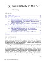
last expression. This definition is more traditional. Let us consider the arbitrarily
oriented elementary area

d

Σ

(Figure 9.1). The orientation direction is determined
by the single vector

n

. The power spectral density passing through the introduced
surface element in the direction of the single vector

s

is defined by the expression:
(9.3)
The ray intensity differs from the spectral
density of the power flow (Poynting’s vec-
tor values) in that the latter value is nor-
malized per unit square while the ray
intensity is additionally normalized per
unit solid angle. This leads to a difference
in the coordinate dependence. For exam-
ple, the power flow decreases with dis-
tance

r

–2

as it recedes from the point
source, while the ray intensity remains
constant.
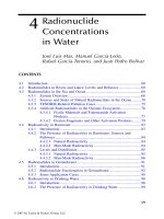
Let us now assign some properties of the ray intensity by examining a ray tube
element in a homogeneous nonabsorbing medium (Figure 9.2), restricted at the ends
by the surface elements and , which are perpendicular to vector

s

. The
power flow through the second surface is defined relative to the power flow through
the first surface by the relation By virtue of the energy conservation
law, however, it must be equal to . Because

where we obtain the equality:
FIGURE 9.1 Oriented elementary area.
n
s
d
Σ

WA
e
() (, ()ω = S)rs Ω


WAdPdAId
ee
() () ( ) ()(,) .ω
π
=
∫
ΩΩ Ω Ω Ω
1
0
S, S S=
3
4
rs
∞∞
∫∫
4
π
dW I d d


() (,) .ω = ⋅
()
rs ns ΣΩ
FIGURE 9.2 Ray tube element in a
homogeneous, nonabsorbing medium.
d
Σ
1
d
Σ
2
ss
dΣ
1
dΣ
2
Iddrs
111
,
()
ΣΩ
Iddrs
222
,
()
ΣΩ ddΣΩ
22
=
dd r ddΣΣ ΣΩ

21
2
11
= r = −||,rr
21

TF1710_book.fm Page 242 Thursday, September 30, 2004 1:43 PM
© 2005 by CRC Press

Transfer Equation of Radiation

243

(9.4)
which expresses the ray intensity constancy along the ray. In differential form, this
property of the ray intensity can be written as the transfer equation:
(9.5)
in a homogeneous, nonabsorbing medium.
Let us now study the changes in ray intensity with wave reflection and refraction
on the interface of transparent media. The energy conservation law requires the
equality on the interface.
The sense of the subscripts introduced here is the same as that used for the wave

θ

r

=

θ

i

and
(Snell’s law), as well as the relations

δΩ

r

=

δΩ

i

=



,
, and The differentiation result follows from Snell’s
law: . Therefore,
(9.6)
The ray intensity of the reflected waves is connected with the ray intensity of the
incident waves by the obvious relation:
(9.7)
Here, the reflective coefficient corresponds to any polarization and is defined by the
half sum of reflective coefficients in the case of nonpolarized waves (compare with
Equation (8.18)). Thus, we obtain the following expression for the ray intensity of

reflected waves:
(9.8)
At a negligibly small coefficient of reflection, we find that The last
expression is generalized by the equation for the value:
(9.9)
IIrr
21
()
=
()
,
dI
d
I
s
= ⋅∇
()
=s 0
IddI ddIdd
ii irr r
cos cos cosθθθΣΩ ΣΩ ΣΩ=+
tt t
εθ εθ
12
sin sin
i
=
t
sinθθϕ
ii i

dd
ddd
tttt
Ω = sinθθϕ dd
ti
ϕϕ= .
εθθεθθ
12
cos cos
ii tt
dd=
III
irt
εεε
112
=+.
IF I
rii
=
()
θ
2
.
IFI
tii
= −
()







ε
ε
θ
2
1
2
1
II
ti
εε
21
= .
J
I
const(,)
(,)
()
rs
rs
r
==
ε

TF1710_book.fm Page 243 Thursday, September 30, 2004 1:43 PM
reflection problems in Chapter 3. Further, we will take into account that
© 2005 by CRC Press

244

Radio Propagation and Remote Sensing of the Environment

along the ray for a medium with permittivity that changes slowly (at the wavelength
scale). Note that the stated constancy follows from the geometrical optics approxi-
mation. Let us state once more that we are discussing transparent media — more
accurately, the imaginary part, for which the permittivity is much less than for the
real part. The transparency of the type of medium considered here is particularly
emphasized by the fact that the reflection angle is implicitly assumed to be a real
value for calculation of the solid angle elements.
Note that invariant Equation (9.9) takes place when the geometrical optics
conditions are not observed but the medium or bordering media are in a state of the
thermal equilibrium (see, for example, Bogorodsky and Kozlov

57

or Aspresyan and
Kravztov

58

).

9.2 RADIATION TRANSFER EQUATION

Ray intensity satisfies an equation known as the radiation transfer equation, which
is of the integer–differential type. It derives from consideration of the energy balance
within an elementary volume, represented as a cylinder of length

ds

with unit square
of transverse cross section. Equation (9.5) is an example of such an equation, and
it is correct for a homogeneous nonabsorbing and nonscattering medium. These
processes, together with changes in the ray tube cross section, must be taken into
consideration. The change in ray tube cross section is described by Equation (9.9),
which, in this case, is convenient to rewrite in the form of the differential relation
It describes amplification or attenuation of the ray intensity on the
elementary segment of ray

d

s dependent on the permittivity gradient sign. The
radiation will be weakened over the same distance due to absorption in the medium
itself (for example, in air) and due to absorption and scattering by particles entering
the medium (for example, drops of clouds). The change in radiation intensity caused
by volume sources has to be addressed. Thus, we obtain the following differential
equation:
(9.10)
Here,

Γ

is the absorption coefficient of the medium,

N

is the particle concentration,
and

E

is the volume density of radiation sources.
Let us regard two processes that are important radiation sources. One of them
is the process of rescattering due to particles of radiation coming upon the considered
volume from other (side) directions. The density of the flow incident within the solid
angle element in the direction

s

′

is equal to S

i

=

I

Multiplying by the
value gives us the power flow density scattered in direction

s

at a
distance

R

from the particle. We can obtain the value of the ray intensity reradiated
in direction

s

by integrating over all directions and summing up the contribution of
all the particles inside the volume being considered:
dI I d= (ln ).ε
dI
d
d
d
NIE
t
ss
= −−






+
ln
.
ε
σΓ
rs,.
′

()
′
dΩ
σ
d
R
′
()
ss,
2
dI N d I d(,) () , , .rs r s s rs=
′
()
′
()
′
∫
s
d
4
σ
π
Ω

TF1710_book.fm Page 244 Thursday, September 30, 2004 1:43 PM
© 2005 by CRC Press

Transfer Equation of Radiation

245

The second source of volume radiation is the proper thermal emission of the medium.
We will establish the spectral density value by a rather unusual method. First, we
will consider the thermal radiation of the particles that are in the medium. The
corresponding spectral density is equal to:
on the basis of Equation (8.34). The combined wave power of both polarizations
was taken into account when writing this expression, so the polarization effects are
not discussed here. The appearance of permittivity of the medium as a factor is
rather unexpected; however, it is an expression of Clausius’ law, which connects the
equilibrium intensity in a transparent isotropic medium with the same in a vacuum.
It is now more convenient to examine the spectral density in the oscillation frequency
scale

f

. In this case, 2

π

has to be reduced (recall that

ω

= 2

π

f

).

Now, it is easy to think about how to calculate the radiation of the medium itself.
For this purpose, it is enough to replace the product with absorption coefficient

Γ

in the previous formula. This substitution is a reflection of Kirchhoff’s law for
equilibrium radiation in the ray definition. Thus, we have the ratio:
. (9.11)
Here, is the universal function of temperature and frequency. We substituted
the permittivity for the refractive index, emphasizing the ray character of Equation
(9.11). The subscript with the frequency is introduced to note the spectral character
of the given relation. The universal function indicated here, which is independent
of the physical nature of the substance, is expressed through the Planck or Ray-
we obtain the equation for the value defined by Equation (9.9):
(9.12)
The subscript

f

is introduced here in order to emphasize again that we are discussing
spectral density on the scale of the oscillation frequency but not the circular one;
however, the subscript will be omitted from now on. We note also that

λ

is the
radiation wavelength in a vacuum.

Let us express the differential cross section in terms of the scattering indicatrix
with the help of the relation:
(9.13)

dI R
NkT
d
a
(,) ( )
() () ()()
rs
rr rr
==

Ss
b
ω
σε
πλ
2
2
2
N
a
σ
E
n
T
ω
ωω

ω
Γ
Θ
2
= ()
Θ
ω
()T
sssrs⋅∇
()
++
()
=
′
()
′
()
′
+
∫
JNJN Jd
ftfdf
ΓΩΓσσ
π
,,
4
++
()
N
kT

a
b
σ
λ
2
.
σσψ σψ ψ
dt
d
′
()
=
′
()
=
′
()
′
()
′
=ss ss ss ss,,
ˆ
,, ,
s
A Ω 11
4
.
π
∫

TF1710_book.fm Page 245 Thursday, September 30, 2004 1:43 PM
leigh–Jeans function for the case of radio frequencies (see Chapter 8). As a result,
© 2005 by CRC Press

246

Radio Propagation and Remote Sensing of the Environment

The transfer equation can be rewritten as:
.
(9.14)
It is necessary at this point to make some remarks. The transfer equation we
derived obviously has a geometric–optical character that reveals itself in the inclusion
of the dependence of all parameters on the only coordinate counted over the ray, in
the inclusion of the propagation medium permittivity, and in the label itself — the
ray intensity of the main energetic value. By the way, other labels have been used
for value

I

in the literature: intensity, spectral brightness, simple brightness, energetic
brightness, etc. The deduction itself is not based on the wave and statistical concept
of radiation propagation. In particular, wave interference due to scattering by an
assembly of particles is not considered, but we have introduced, by the simple
summation of the scattered power, the idea of a scattered wave incoherence. More-
over, the waves coming to any point from different directions are also considered
to be incoherent. The integral term and the extinction component coefficient in
Equation (9.14) are written, obviously, using the single scattering approach; conse-
quently, the equation concerns the case of rarefied media. The situation is rather
improved by the substitution of the product for the total cross section per unit

volume; however, it is difficult to determine up to what level of media density the
given substitution works. In the case of small particles (compared to the wavelength),
for which dipole scattering is the primary type, the matter is reduced to the intro-
duction of dielectric permittivity based on the Lorentz–Lorenz formula. This formula
takes into account the mutual polarization of particles as the first approximation
with respect to the density, and the scattering itself is described as scattering by the
density fluctuations.
The most logical deduction of the transfer equation is based on the analysis of
spatial spectral properties of the coherency function. In particular, the ray intensity
is defined as a Fourier transform of this function over the differential coordinates.
We will not examine this problem in detail but refer interested readers to the
appropriate literature.

58

The validity of the transfer equation has been proven by the
fact that the solutions of many problems based on it agree with the experimental data.
Let us point out, as well, that the transfer equation is analogous to the Boltzmann
kinetic equation for the stationary case. Particularly, its integral term is similar to
the collision integral and describes the scattering of light particles (photons) by
heavy particles. It explains why in our case the collision integral is linear with respect
to the ray intensity. Obviously, many methods developed to solve the kinetic equation
can be used to solve radiation transfer problems.

61


Let us now introduce the optical thickness using the formula:
(9.15)

sssrs⋅∇
()
++
()
=
′
()
′
()
′
+
∫
JNJN Jd
tt
ΓΩσσψ
π
ˆ
,,A
4
ΓΓ + −
()




1
2
ˆ
A N
kT

t
b
σ
λ
Nσ
t
τσ() () () ()sssss
s
=+




∫
Γ Nd
t
0

TF1710_book.fm Page 246 Thursday, September 30, 2004 1:43 PM
© 2005 by CRC Press

Transfer Equation of Radiation

247

with the following definition:
(9.16)
Then, the transfer equation can be written down in a dimensionless view:
(9.17)
For transfer problems, we do not raise the question of emission polarization.

This problem demands a special approach that considers scattering effects. The
polarization of scattered radiation can differ from the polarization for incident
radiation, and, generally speaking, it should be taken into account by adding the
intensities of differently polarized waves with the same weight, as was done with
Equation (9.12). The situation gets even more complicated when radiation transfer
in anisotropic plasma is taken into account. In this case, it is possible to have partial
transformation of waves of one type to the other (for example, ordinary into extraor-
dinary) upon scattering. In order to describe this, we would have to put together a
system of linked transfer equations, including pointed transformations. We will not
go into the details of this problem but instead refer readers to the appropriate
literature.

58

Here, we will note only that polarization phenomena do not play a crucial
role in our further discussions; therefore, we will consider the formulated equations
above to be quite sufficient for our aims.

9.3 TRANSFER EQUATION FOR A PLANE-LAYERED
MEDIUM

The approach for a plane-layered medium is appropriate for many of the cases we
will examine further. We will suppose that all the medium properties (absorption,
scattering) depend on the z-coordinate. We will also assume that all rays are straight
at an angle

θ

to the z-axis. For the atmosphere of Earth, for example, this means
that we can ignore its spherical stratification and neglect the ray bending due to

refraction. We are entitled to assume that and to write:
(9.18)
Here,
(9.19)
c
Ns
N
t
()
ˆ
() ()
() () ()
.s
s
sss
t
=
+
A σ
σΓ
dJ
d
Jc J d c
kT
b
τ
ψτ
λ
π
+ −

′
()
′
()
′
= −
()
∫
ss s,, .Ω 1
2
4
s = zcosθ
µ ψ
dJ
dz
Jc Jz d c
k
+ −
′
()
′
()
′
= −




(,, (z) z, z)ss s Ω 1
bb

T
λ
π
2
4
.
∫
zNd
t
zzzzz,
z
()
=
′
()
+
′
()
′
()




′
=
∫
Γσµ θ
0
cos .

TF1710_book.fm Page 247 Thursday, September 30, 2004 1:43 PM
© 2005 by CRC Press

248

Radio Propagation and Remote Sensing of the Environment

We also represented the coordinate dependence of the scattering indicatrix, empha-
sizing the possible types of particle changes and their shape from the layer to layer.
Let us now consider a simple example of solving the transfer equation — an
absorbing atmosphere with no scattering particles. The albedo is equal to zero, so

c

= 0. We assume that the radiation comes from the semispace toward a receiving
point on Earth (z = 0). In this case, the transfer equation can be written in the form:
(9.20)
The minus before the first summand on the left-hand side is here because we are
concerned with radiation propagating in the direction of negative values of z. The
solution of this equation at the formulated boundary condition is:
(9.21)
At z = 0, the spectral density of the ray intensity that we obtained should be multiplied
by the effective area of the antenna directed at angle

θ

to the zenith and integrated
over all possible directions. The antenna itself is assumed to have a narrow pattern,
which permits us to neglect the

µ

change during the integration. As a result, we
obtain the spectral density of power and then the brightness temperature. In fact, it
will be the antenna temperature value, but both temperature values, as was already
mentioned, practically coincide at a rather acute antenna pattern. Thus,
(9.22)
Let us now study the radiation of a layer of thickness

d

situated in the altitude
interval . The temperature inside the layer is assumed to be constant,
and we will also assume an absence of absorption in the layer environment of the
frequency waves being studied. It follows from Equation (9.22) that, in this case:
(9.23)
− +=
()
→
→∞
µ
λ
µ
dI
dz
I
kT
I
b

2
0,.z,
z
Iz
k
eTedzz d
b
zz
z
z
,,(
)
µ
λ
µµ
()
=
′
=
−
′
∞
∞
∫
∞
2
0
Γ z) z .
(z
∫∫

TTedz T d
z

() ( ( expµ
µµ
µ
== −
′
()
′


−
∫
11
0
ΓΓz) z) z z
z






∞
∫∫
∞
d
z
z.

00
z,z
00
+




d

T
T
dd T

() ( expµ
µµ
= −
′
()
′








=
∫

ΓΓz) z z z
z
z
0
1
1−−






−
()
+
∫
e
d
d
τ µ,
,
z
z
0
0

TF1710_book.fm Page 248 Thursday, September 30, 2004 1:43 PM
© 2005 by CRC Press

Transfer Equation of Radiation

249

where the optical thickness is defined by the integral within the radiating layer:
This equation agrees with Equation (8.32) and conveys the fact that the reflection
effects on the interfaces are neglected.
Let us investigate further the radiation of a semispace by considering a soil with
constant temperature radiating into an absorbing atmosphere. To simplify the
problem, we will concentrate on the analysis of radiation propagation in the vertical
direction relative to the boundary; that is, we will assume that

µ

= 1. Equation (9.21)
can be used to determine the radiation ray intensity of the soil at the surface; however,
we should not ignore the fact that the soil permittivity differs substantially from
unity, which is why it is necessary to derive an equation for value

J

that describes
the radiation inside the soil. Thus, we will have:
(9.24)
Equations (9.24) and (9.8) define the boundary condition for the ray intensity
of atmospheric radiation. The transfer equation gives us the solution:
(9.25)
The constant

T

0

is fixed from the boundary condition:
(9.26)
The expression for the ray intensity of the soil and atmosphere at altitude z above
the interface is obtained. Let us suppose that the radiation is received onboard a
satellite at an altitude much greater than the thickness of the atmosphere. This gives
us the opportunity to regard z

→



∞

in our formulae, and, accordingly,

z



→



z

∞

. The

corresponding expression for the brightness temperature gives us:
τ µ
µ
(,)dd
d
=
′
()
′
+
∫
1
Γ zz.
z
z
0
0
T
g
J
IkT
g
g
g
bg
()
()
.0
0
2

==
ε
λ
Iz
k
eT Tedz
a
b
z
a
z
z
(.z)




=+
′








−
′
∫

λ
2
0
0
I
I
F
kT
F
a
g
g
bg
()
()
.0
0
11
2
2
2
= −
()
= −
()
ε
λ
TT d T
gg a
= −









+ −
∞
∫
κ exp ( ( ( expΓΓΓz) z z) z)
0
′′
()
′








∞∞
∫∫
zzz.
z
dd
0

TF1710_book.fm Page 249 Thursday, September 30, 2004 1:43 PM
© 2005 by CRC Press

250

Radio Propagation and Remote Sensing of the Environment

The first summand describes the soil radiation attenuated by absorption in the
atmosphere, and the second one describes the sum of the proper radiation of the
atmospheric layer, also attenuated by absorption; however, the represented formula
is not complete, as it excludes the atmospheric summand directed downward toward
the soil border, reflected upward, and then attenuated by absorption in the atmo-
sphere. The intensity of descending radiation on the interface is easily defined from
Equation (9.21) as follows:
Now, it is easy to take into account the resulting contribution in the brightness
temperature and to obtain as a result:
(9.27)
The known equation is obtained for the soil brightness temperature in the absence
of atmospheric absorption. The solution to the total problem could be obtained at
once if we were to use the more complete boundary condition:
(9.28)
instead of Equation (9.26).

9.4 EIGENFUNCTIONS OF THE TRANSFER EQUATION

Let us now consider a medium in which particles put into it influence predominantly
radiation propagation. This means that the absorption in the medium itself is rather
small (i.e., assume

Γ

= 0). To simplify the problem, we also assume a small variance
in permittivity from unity; hence, it is sufficient to assume that

ε

= 1. In this case,
the function is a constant value which means that the scattering particles
are invariable in all space and the albedo does not depend on spatial coordinates.
So, the transfer equation can now be written as:
(9.29)
I
k
Tdd
a
b
↓
= −
′
()
′









∫
() ( ( exp0
2
0
λ
z) z) z z
z
ΓΓ
′′
∞
∫
z.
0

TTT eFed
gg a
zz

=+ +







−
∞
∫
κ ((

((
z) z) z
z) z)
Γ
2
0









−
∞
e
z
.
I
k
TFT ed
a
b
gg
z
↑
−
∞

=+






∫
() ( (
(
0
2
2
0
λ
κ z) z) z
z)
Γ


c()
ˆ
z = A
µ ψ
λ
π
dI
dz
IIzd
kT

b
+ −
′
()
′
()
′
= −
()
∫
ˆ
,,
ˆ
.AAss s Ω 1
2
4

TF1710_book.fm Page 250 Thursday, September 30, 2004 1:43 PM
© 2005 by CRC Press

Transfer Equation of Radiation

251

Equation (9.29) is an integer–differential equation in which the right-hand side
plays the role of an impressed force. Let us now consider the question: What are
the eigenfunctions of the homogeneous equation (i.e., the equation with an impressed
force equal to zero)? Naturally, these functions will depend on the scattering indi-
catrix type. To simplify the problem, we will assume the simplest case of isotropic
scattering indicatrix; that is,

(9.30)
In this case, the ray intensity will depend on only the z-coordinate and angle

θ

or
value

µ

. Then, it is possible to perform the integration in Equation (9.29) with respect
to azimuth angle , and the homogeneous transfer
equation can be written in the form:
(9.31)
We will now search for the solution in terms of the separation of variables
method:

60


(9.32)
The functions are eigenfunctions and

ν

represents eigenvalues. As eigenfunc-
tions are determined accurate to constant multiplier, it is convenient to introduce the
normalization:
(9.33)
Then, it follows from the transfer equation that:

(9.34)
The direction cosine

µ

varies within the interval [–1,+1]. If the eigenvalue

ν

lies
outside this interval, then the unknown eigenfunctions are represented in the form:
(9.35)
ψ
π
′
()
=ss,.
1
4
′′
=
′′ ′
=
′′
ϕθθϕµ ϕ(sin )dddddΩ
µ
µ
µµµ
dI z
dz

Iz Iz d
,
,
ˆ
,.
()
+
()
−
′
()
′
=
−
∫
A
2
0
1
1
Iz e
z
νν
ν
µ φ µ(, ) () .=
−
φ µ
ν
()
φ µµ

ν
() .d =
−
∫
1
1
1
()()
ˆ
.ν µ φ µ
ν
ν
− =
A
2
φ µ
ν
ν µ
ν
()
=
−
ˆ
.
A
2
1

TF1710_book.fm Page 251 Thursday, September 30, 2004 1:43 PM
© 2005 by CRC Press

252

Radio Propagation and Remote Sensing of the Environment

The eigenvalues themselves are defined from the condition of the normalization,
Equation (9.33), and we obtain the following equation:
. (9.36)
This other view of the equation form is more transparent for our analysis:
. (9.37)
Because the albedo value is less than unity and based on the hyperbolic tangent
behaviors, we can state that this equation has two real roots differing only in sign.
Let us designate them as ±

ν

0

. We exclude from our consideration the roots on the
imaginary axis because doing so would require a more detailed analysis.

60

It is a simple matter to estimate the values of the roots in extreme cases. If
, then

ξ

>> 1, and
(9.38)

The value

ξ

is small in the other extreme case of the albedo approaching unity
(1 – << 1). The following equation is obtained from the hyperbolic tangent
expansion:
. (9.39)
Also, we have established the existence of two modes:
(9.40)
from the discrete spectrum of eigenfunctions. The eigenvalues of this spectrum are
situated on the real semi-axis [–1,–] and [+1,+].
The situation becomes rather more complicated when we include [–1,+1] in the
discussion. First, Equation (9.34) cannot be divided by

ν

–

µ

in all cases. Second,
we must take into account the functional equality x

δ

(x) = 0, which allows us to add
the summand to the obvious solution of Equation (9.34). Thus, the
continuous spectrum modes from the class of generalized functions

61,62

are added
ˆ
ln
Aνν
ν2
1
1
1
+
−
=
tanh
ˆ
,
ˆ
ξ
ξ
ξ
ν
==A
A
1
ˆ
A<<1
11
12
0
2

ν
≅≅−
−
tanh
ˆ
.
ˆ
A
A
e
ˆ
A
1
31
0
ν
≅−(
ˆ
)A
φ µ
ν
ν µ
ν±
()
=±
± −
0
0
0
2

1
ˆ
A
Λ()( )νδν µ−

TF1710_book.fm Page 252 Thursday, September 30, 2004 1:43 PM
© 2005 by CRC Press

Transfer Equation of Radiation

253

to the already found functions of the discrete spectrum. In general, they can be
written in the form:
(9.41)
where

P

represents the principal value. Let us recall that generalized functions have
meaning not per se but under the integral sign; it is important to understand the
principal value sign and delta-function in this regard. The normalization condition
leads to the definition:
(9.42)
Let us point out that the principal representation of function

Λ

(

ν

) corresponds
to the representation of the second summand via the integral. Its representation
through the logarithm of Equation (9.42) is related to the case when

ν

lies inside
the integration interval; in this case, we should use the rules of principal value
calculations. In other cases, it is necessary to introduce the substitution:
which means that
These eigenfunctions possess the properties of orthogonality and completeness
over the entire segment . The orthogonality is defined
with weight

µ

; that is,
(9.43)
The norms of discrete modes are connected by the equality and
the value:
(9.44)
Calculation of the norm in the case of a continuous spectrum becomes more
complex due to the peculiarities of eigenfunctions, particularly because they are not
φ µ
ν
ν µ
νδν µ
ν

()
ˆ
()( ),=
−
+ −
A
2
1
P Λ
Λν
ν µ
ν µ
νν
ν
()
= −
−
= −
+
−
−
∫
1
2
1
2
1
1
1
1

ˆˆ
ln .
AA
P
d
ln ln ,
1
1
1
1
+
−
⇒
+
−
ν
ν
ν
ν
Λ() .ν
0
0=
(, )−∞ <<+∞−≤≤+z 11µ
µ φ µ φ µµ νν
νν
() () , .
′
−
=
′

≠
∫
d 0
1
1
NN() ()− = −νν
00
Ndν µ φ µµ
νν
ν
ν0
2
00
2
0
2
0
11
21
()
==
−−




−
(
()
ˆ

(
ˆ
)AA
))
−
∫
.
1
1

TF1710_book.fm Page 253 Thursday, September 30, 2004 1:43 PM
© 2005 by CRC Press

254

Radio Propagation and Remote Sensing of the Environment

functions with the integrated square. For completeness, any “good” function can be
represented as:
. (9.45)
The components of the discrete spectrum are easily found. For example, the first of
them is defined from the obvious equality:
(9.46)
By analogy, the spectral density has to satisfy the relation:
(9.47)
Further calculations are more complex due to the fact that the result of integration
depends on the order of integration due to the singularity of the integrands. Substi-
tution in Equation (9.47) of the obvious expressions of the eigenfunctions provided
in Equation (9.41) gives us:
The Poincare–Bertrand formula now becomes very useful:

63

. (9.48)
Here,

L

is a smooth contour on the plane of complex variable

t

. The points

t

0

and

t

1

are on this contour. This formula now gives us:
ff f f dµ φ µ φ µ νφ µ ν
νν ν
()
=
()

+
()
+
′
() ()
′
+ −−
′
 
00
00
−−
∫
1
1
µµφ µµ µφ µµ ν
νν
fdf dfN
() ()
=
()
=
()
++
−
∫
00
0
2
00

1
1

.
−−
∫
1
1


fN f d f dνν µµφ µµ νφ µ ν µ φ µ
ννν
() ()
=
() ()
=
′
() ()
′
(
′
))
−−−
∫∫∫
dµ .
1
1
1
1
1

1

N
f
P
d
P
f
dνν ν
ν
ν
µ
µ ν
µ νν
ν µ
()
=
()
−
()
−
′′
()
′
−
Λ
2
2
4
ˆ

A


′′
+
+
()
′
−
′′
()
′
−−
∫∫
ν
ν
ν
ν
µ ν
µ νν
ν
1
1
1
1
2
4
1
ˆ
A



f
dP P
f
−−
−−
∫∫
µ
µd .
1
1
1
1
P
dt
tt
P
tt
tt
tt dt P
tt
P
−
()
−
= −
()
+
−

0
1
1
2
00 1
0
1
ϕ
πϕ
ϕ,
,
ttt dt
tt
LLLL
,
1
1
()
−
∫∫∫∫

TF1710_book.fm Page 254 Thursday, September 30, 2004 1:43 PM
© 2005 by CRC Press

Transfer Equation of Radiation

255

(9.49)

9.5 EIGENFUNCTIONS FOR A HALF-SEGMENT

The eigenfunctions of the transfer equation discussed previously apply to the case
of infinite space; that is, we considered the case when the radiation propagation
direction could be any (–1

µ

1). However, the case of semispace occurs frequently
when the direction of radiation propagation is restricted by the limits (0 µ

1). The
opposite case of negative directions is similar. The transfer to the half-segment (0
µ 1) demands, generally speaking, reworking the problem because the eigenfunctions
examined in the previous part were defined on a full segment (–1 µ 1). Luckily, we
can prove that the functions defined by us have the property of completeness for the
half-segment, too.
61
Hence, it is not necessary to introduce new functions, but the
orthogonality problem does require some special attention. It is necessary to intro-
duce another weight function W(µ), which satisfies the singular equation:
(9.50)
and the condition:
(9.51)
By using:
(9.52)
we can reduce the previous equation to the uniform equation of Carleman:
(9.53)
The solution to Equation (9.53) must satisfy the condition:
(9.54)

N νν ν
π
νν
νν
()
=
()
+








= −
+
−
Λ
2
22
2
4
1
2
1
1
ˆˆ
ln

AA
νν
π
ν






+








2
22
2
4
ˆ
.
A
ˆˆ
AAν
µµ
ν µ

νν
ν
22
0
1
P
Wd
W
()
−
+
() ()
=
∫
Λ
Wd()
.
µµ
ν µ
0
0
1
1
−
=
∫
WV() ()µ ν µµ= −
()
0
avVv AP

Vd
v
av
v
v
() ()
−
()
−
=
()
=
()
∫
ˆ
,.
µµ
µ
0
1
0
2Λ
Vd() .µµ=
∫
1
0
1
TF1710_book.fm Page 255 Thursday, September 30, 2004 1:43 PM
© 2005 by CRC Press
256 Radio Propagation and Remote Sensing of the Environment

The theory of singular integral equations is covered in detail in the well-known
monograph of Musheleshvily.
63

We can now see that, according to our method, the solution has the form:
(9.55)
We can also write the solution in the form:
(9.56)
where
. (9.57)
Integration by part allows us to state that:
. (9.58)
The tables for this function can be found in Case and Zweifel.
60
The relations
(9.59)
are found to be useful where the function:
(9.60)

V
Ce
a
P
d
µ
µµπ
τ µ
π
νν
ν

τ µ
()
=
−
()()
+
=
()
1
1
222
ˆ
,()
()
A
Θ
−−
=
∫
µ
ν
π
ν
0
1
,tan()
ˆ
()
.Θ
Α

a
W
X
N
µ
µ ν µµ
µ
()
=
−
()()
()
ˆ
,
A
3
2
0
2
Xz
z
P
zdz
zz
() exp=
−
′
()
′
′

−








∫
1
1
1
0
1
π
Θ
Xz
z
z
zzzdz
()
= − +
′
−
′







′
−
′
()
′
exp
ˆˆ
ln
AA
2
1
1
2
2
NNz
′
()








∫
0
1

XzX z
z
z
XX
()
−
()
=
()
−−
()
−
()
= −
ˆ
(
ˆ
)( )
,
Λ
1
0
22
00
A ν
νν
111
21 1
0
2

0
2
0
2
−−
−−
(
ˆ
)
(
ˆ
)( )
A
A
ν
νν
ˆ
ˆ
Λ z
zd
z
()
= −
−
−
∫
1
2
1
1

A µ
µ
TF1710_book.fm Page 256 Thursday, September 30, 2004 1:43 PM
© 2005 by CRC Press
Transfer Equation of Radiation 257
is determined as the function of complex variable z (compare with Equation (9.42)),
and
(9.61)
Let us point out that the first expression in Equation (9.59) is valid on the entire
complex plane z with the section along the real axis on the segment from zero to
the unity. It can be written as:
(9.62a)
on the section itself. The last result is derived with the help of Sohotsky–Plemelj
formula.
63
The table of normalizing integrals is cited in Reference 60. Equation (9.61) is
very helpful for its deduction. The unknown integrals can be represented as:
(9.62b)
(9.62c)
(9.62d)
. (9.62e)
Wd
X
()
().
µµ
ν µ
ννν
−
= −−

()
∫
1
0
0
1
XX
N
A
() ( )
()
(
ˆ
)
µµ
µ
µ
ν µ
− =
−−
()
1
1
0
22
φ µ φ µµµ ν
ν
ν
δν ν
φ

νν
ν
() () () ()
()
,
′
+
∫
= −
′
()
Wd W
N
0
1
0
0
11
0
∫
=() () () ,µ φ µµµ
ν
Wd
φ µ φ µµµ νν ν φ ν
νν ν−−
∫
= −
()
00
0

1
0
() () ()
ˆ
(),Wd XA
0

φ µ φ µµµ
ν
ν
νν±+
∫
=






±
()
00
0
1
2
0
() () ()
ˆ
Wd X∓
A

2
0
,,
() () ()
ˆ
(),φ µ φ µµµ
νν
ν
νν− +
= −
∫
0
0
1
Wd X
A
4
0
φ µ φ µµµ
ν
φννν ν
νν ν−
′
−
=
′
′
()
+
()

−() () ()
ˆ
()Wd X
A
2
0
0
11
∫
TF1710_book.fm Page 257 Thursday, September 30, 2004 1:43 PM
© 2005 by CRC Press
258 Radio Propagation and Remote Sensing of the Environment
9.6 PROPAGATION OF RADIATION GENERATED ON
THE BOARD
Let us now consider the problem of radiation by sources given on the layer board
as a function This means that the coefficients of the ray intensity expansion:
(9.63)
are found from the boundary condition:
(9.64)
The standard procedure leads to the relations:
(9.65)
In particular, note that at zero albedo (i.e., no scattering)
and the ray intensity is:
(9.66)
The obtained formulae are rather complex. They can be simplified a little in the
directed radiation source given by the formula I
0
(µ) = however, even
in this case the general analysis is not simple, so we will limit ourselves to the study
of an extreme case.

The first summand in Equation (9.63) becomes dominant at a sufficient distance
from the source, in this case from the interface, as . Then, at z >> 1:
(9.67)
I
0
().µ
Iz b e b e d
z
z
(, ) () () ()µ φ µ νφ µ ν
ν
ν
ν
ν
=+
−
−
∫
0
0
1
0
0
Ib b dI(,) () () () ().0
00
0
1
0
µ φ µ νφ µ ν µ
νν

=+ =
∫
b
X
IW d
b
0
2
0
2
0
0
0
1
4
0
= −
()
′
()
′
()
′
()
′
∫
A νν
µµφ µµ
ν
ν

,
( ))
() ()
.=
′
()
′
()
′
()
′
∫
ν
νν
µµφ µµ
ν
WN
IW d
0
0
1
φ µ
ν
0
0() ,=
φ µ δν µ
ν
() ( ),= − NbI() , () (),νν ν ν==and
0
IIe

z
() () .µµ
µ
=
−
0
δ µµ−
()
0
;
ν
0
1≥
Iz
V
X
e
z
,.µ
µ
ννµ
ν
()
≅−
()
()
−
()
−
0

00
0
TF1710_book.fm Page 258 Thursday, September 30, 2004 1:43 PM
© 2005 by CRC Press
Transfer Equation of Radiation 259
It is easy to determine that the distance over which the radiation propagates can be
obtained by the equation:
(9.68)
We note that here N represents the particle concentration. For a given concentration
and cross section, this distance is equal to:
(9.69)
When the albedo tends to unity (in the case of no absorption), the discrete eigenvalue
tends to infinity ( ), which means that the medium is filled up with radiation
for which the intensity does not depend on coordinates z and µ at a sufficient distance
from the source and tends to the value True, infinite time is needed
to reach this value in the whole volume.
9.7 RADIATION PROPAGATION IN A FINITE LAYER
The problem of radiation propagation in the semispace occupied by scattering
elements was discussed in the previous section. Closer to reality is the problem of
radiation propagation in a layer of finite thickness d. The difference from the previous
consideration is that the condition:
(9.70)
should be added to the boundary condition of Equation (9.64). The appearance of
this second boundary condition allows us to include backward radiation in our
analysis. Thus, the solution of the transfer equation should be represented as the sum:
(9.71)
The source of radiation will be assumed, for the sake of simplicity, to be in the form
of a delta-function. We then obtain two equations, adding up and subtracting the
boundary conditions:
Nd

t
′
()
′
()
′
=
∫
zzz
z
0
σν
0
0
.
z
0
=
ν
σ
0
N
t
.
ν
0
→∞
Iz V(, ) ( ).µµ→
0
INd

ddt
d
zzzzz,, ,µµ σ
()
=< =
′
()
′
()
′
∫
00
0
Iz b e b e
b
zz
,() ()µ φ µ φ µ
ν
ν
ν
ν
ν
()
=+ +
+
′
()
+
−
−−00

0
0
0
0
φφ µ ννφµ ν
ν
ν
ν
ν
′
−
′
−
′
′
′
+ −
′
()
′
∫∫
() () .ed b ed
zz
0
1
0
1
TF1710_book.fm Page 259 Thursday, September 30, 2004 1:43 PM
© 2005 by CRC Press
260 Radio Propagation and Remote Sensing of the Environment

, (9.72)
which are equivalent to the boundary conditions in Equations (9.64) and (9.70). We
can introduce the following functions for brevity:
(9.73)
and the following relations are useful:
(9.74)
They follow from Equation (9.62a) for normalizing integrals. If we take into account
the properties of eigenfunction due to changes in the argument and subscript sign,
then the following relations can be obtained:
. (9.75)
The equations of orthogonality lead to the relations:
(9.76)
δ µµ µ ν µ ν
νν
−
()
=+
′
()
′
±± ±
′
±
∫
00
0
1
0
BBdΦΦ() ()
Bbbe B b be

d
d
000
0
0
±+− ±
=± = ±−
z
z
ν
ν
νν
νν ν,()()(),
,
Φ
±± −
−
=±() () ()
,,
,
µ φ µ φ µ
νν νν
νν
00
0
e
d
z
VdXVd() ()
ˆ

,()() ,µ φ µµ
ν
ν µ φ µµ
νν±
=±
()
=
0
0
0
0
1
2
0∓
A
∫∫∫
∫
− = −
()
≥
0
1
0
1
2
0VdX() ( )
ˆ
,.µ φ µµ
ν
νν

ν
A
B
VBXed
X
d
0
0
0
1
0
2
±
±
−
′
= −
()
′
()
−
′
()
′′
∫
A
µ νν νν
νν
ν
∓

z
000
0
()
−
()








−
∓ Xe
d
ν
ν
z
B
WN
WB
X
±±
=
() ()
−
()
()

() ()
ˆ
ν
νν
ν
µ φ µ
νν ν
ν000
2
0
2
0
∓
A
22
4
0
2
0
0
νν
νν ν
νν
νν
ν
+
()
+
′
+

′
−
′
()
′
()
−
±
e
XBe
d
z
∓
∓
ˆ
A
−−
′
′′
∫
z
d
d
ν
νν.
0
1
TF1710_book.fm Page 260 Thursday, September 30, 2004 1:43 PM
© 2005 by CRC Press
Transfer Equation of Radiation 261

If Equation (9.75) is substituted here, then we obtain inhomogeneous Fredholm
integral equations of the second order with respect to the functions , and the
method of consecutive approximations is one to solve them. It is especially effective
in the case of a thick layer, when z
d
>> 1, when the integral terms are small and
can be dropped in the approximation. The zero approximation gives us the following
equations:
(9.77)
Here,
(9.78)
Analogously,
(9.79)
We will now restrict ourselves to the case of an albedo close to unity. Then, we can
assume that and use:
(9.80)
In this approximation, we have:
(9.81)
It is easy to see that we arrive at the previous result in the case of a layer of infinite
thickness ( ).
For the amplitudes of the continuous spectrum, the summand with should
be taken into account only close to the right boundary of the regarded layer. We can
show that in this area the corresponding summand has the order of smallness.
B
±
()ν
b
VX
U
eb

VX
d
0
00
00
0
0
22
0
+ −
= −
()()
()
= −
()
−µ ν
νν
µ ν
ν
z
,
00
00
0
()
()
−
νν
ν
U

e
d
z
,
UXeX e
dd
νν ν
νν
0
2
0
2
0
00
()
=
()
−−
()
−
zz
.
b
V
WN
X
ν
ν µ
νν
ν µ φ µ

νν ν
ν
()
=
()
−
()()
+
−
0
00 0
2
0
2
() ()
ˆ
A
00
00
22
0
0
()
+









−
()
=
−
()()
,
ˆ
ννν
ν
νν
ν
U
e
b
d
z
A XXX V
UWN
e
d
ννµ
ννν νν
ν
000
00
()
−
()()

+
−
()()() ()
.
z
ν
0
1>>
XU
d
ν
ν
ν
ν
ν
0
0
0
0
2
0
12
()
≅−
()
≅







,.sinh
z
b
V
z
eb
V
d
d
0
0
0
0
0
0
+ −
=
()






= −
()
µ
ν

µ
ν
sinh sinh
z
,
zz
e
d
d
ν
ν
0
0






−
z
.
z
d
>> ν
0
b()−ν
ν
0
1−

TF1710_book.fm Page 261 Thursday, September 30, 2004 1:43 PM
© 2005 by CRC Press
262 Radio Propagation and Remote Sensing of the Environment
The second summand in the first expression of Equation (9.79) is also small;
therefore in this case, we can assume that in zero-order approximation,
and
(9.82)
As before, we can neglect the components of the continuous spectrum far away from
the sources and write the ray intensity as:
(9.83)
The ray intensity turns to zero, in the given approximation, at z = z
d
. The approxi-
mation is exactly correct for µ < 0, reflecting the absence of radiation entering from
outside. For µ > 0, describing radiation coming out, it is true if we neglect the values
of the order of at least or .
Now, let us define the value of radiation coming out at the boundary z = 0. For
this purpose, it is necessary to calculate the ray intensity , which in this
case is equal to:
.
As pointed out in Reference 60, this last integral is computed analytically and is
equal to:
(9.84)
Taking into account the adopted approximations, we have:
(9.85)
b()− =ν 0
b
V
WN
V

VN
()
() () () ()
ν
νν µ
νν
φ µ
ν µ
νν
φ
ν
≅
()
()
≅
()
00
0
0
νν
µ
0
()
.
Iz V
z
d
d
(, )µµ
ν

ν
≅
()
−
()











0
0
0
sinh
z
sinh
z



.
ν
0
1−

z
d
−1
I(, )00µ<
IV
d
WN
00 1
0
00
0
0
,
() ()
µµν
φ µ φ µ νν
νν
νν
<
()
=
()
+
<
()()
11
∫









φ µ φ µ νν
νν νµ
ν µ ν
νν
<
()()
=
−
−
()()
0
11
0
0
00 0
d
WN
X
() ()
++
−
()









∫
1
0
0
1
µµµX()
.
I
V
X
00
0
0
,
()
.µ
µ
µµµ
<
()
=
()
−
()
TF1710_book.fm Page 262 Thursday, September 30, 2004 1:43 PM

© 2005 by CRC Press
Transfer Equation of Radiation 263
9.8 THERMAL RADIATION OF SCATTERERS
Now, let us assume thermal radiation of the scatterers occupying the semispace. The
peculiarity here is that the processes of volume radiation are accompanied by the
processes of volume scattering. We need to solve the equation:
(9.86)
To simplify the problem, one can assume that the temperature of the particle is
constant. This allows us to search for the problem solution in view of the sum:
(9.87)
It is easy to see that the first summand in the written solution satisfies Equation
(9.86) on the right-hand side. The two other summands define the solution of the
homogeneous transfer equation with the condition that it tends to zero at z → ∞.
The whole solution has to turn to zero on the boundary of the semispace, which
reflects the fact of the radiation coming back from the left. The condition:
occurs on this basis. The standard procedure for use of the orthogonality conditions
allows us to obtain:
(9.88)
The integral in the second formula can be computed with the use of Equations (9.40)
and (9.61); however, it is not necessary to do so, as further on we will be interested
in the value , which describes the intensity of the radiation coming out,
thereby determining the emissivity of the system of scatterers (medium) under
consideration. It follows from our formulae that:
µ
µ
µµµ
λ
dI z
dz
Iz Iz d

kT
b
,
,
ˆ
,
ˆ
()
+
()
−
′
()
′
= −
()
A
A
2
1
2

−
∫
1
1
Iz
kT
be b e
b

z
z
(, ) () () ()µ
λ
φ µ νφ µ
ν
ν
ν
ν
=+ +
−
−
∫
2
0
0
1
0
0
ddν.
bbd
kT
b
0
2
0
1
0
φ µ νφ µ ν
λ

νν
() ()+
()
= −
∫

b
kT
X
b
kT
WN
W
bb
0
00
2
2
2
=
()
= −
′
(
ˆ
,()
() ()
Aννλ
ν
λ

ν
νν
µ
))
′
()
′
∫
φ µµ
ν
d .
0
1
I(, )00µ<
κ µ
ν µ ν
µµ
φ µ φ µ
νν
<
()
=+
+
()
()
−
′
()
′
<

()
′
()
01
1
0
00
X
Wd
ννν
νν
d
WN() ()
.
0
1
0
1
∫∫
TF1710_book.fm Page 263 Thursday, September 30, 2004 1:43 PM
© 2005 by CRC Press
264 Radio Propagation and Remote Sensing of the Environment
The inner integral is calculated according to Equation (9.84). It is necessary to take
into account Equations (9.51) and (9.61) in the further calculations, and we obtain:
(9.89)
Note that the obtained formula satisfies the extreme conditions. At albedo equal to
zero, and
, (9.90)
and . This medium behaves as a black body. When the albedo is equal to
unity, , and the emissivity becomes equal to zero, which is natural. It is

necessary to point out that the absence of reflections from the interface is assumed
implicitly in our consideration, which means that the emissivity becomes equal to
unity.
9.9 ANISOTROPIC SCATTERING
The model we used for isotropic particle scattering is an idealization of natural
processes and should not be regarded too critically; however, it does give us the
opportunity to describe correctly many versions of the phenomenon on the basis of
a rather simple model. It is natural that further refinement of the model requires the
inclusion of scattering anisotropy. We will briefly analyze the process of taking into
account anisotropy for the rather simple case of particles for which the scattering
indicatrix depends only on the angle between the directions of incident and scattered
waves. This angle is defined by the scalar product . The ray intensity
will not depend on azimuth angle ϕ for this assumption. The homogeneous transfer
equation can be written as:
(9.91)
In this approach, the scattering indicatrix is represented as the expansion over the
Legendre polynomial:
(9.92)
κ µ
ν µµ
<
()
=
+
()
−
()
0
1
0

X
.
ν
0
1=
Xz
z
()=
−
1
1
κ
µ()
= 1
ν
0
→∞
()cos
′
⋅ =ss γ
µ
µ
µ ψ µ
π
dI z
dz
Iz Iz d
,
,
ˆ

,.
()
+
()
−
′
⋅
()
′
()
′
=
A
2
0
4
ss Ω
∫∫
ψψγ γ
′
⋅
()
=
()
=
()
=
∞
∑
ss cos cos .aP

nn
n 0
TF1710_book.fm Page 264 Thursday, September 30, 2004 1:43 PM
© 2005 by CRC Press
Transfer Equation of Radiation 265
The following equality is valid in the chosen coordinate system:
(9.93)
Here, the primed angles correspond to the direction of the incident wave and the
nonprimed angles to the scattering direction. In an addition theorem,
44
(9.94)
where are Legendre associated polynomials, and Let us
substitute expansion Equation (9.92) in Equation (9.91) and take into account Equa-
tion (9.94). Then, it is easy to perform the integration over , using the property
of axis symmetry for ray intensity. As a result, the sum connected with Legendre-
associated polynomials will disappear, and the transfer equation is as follows:
(9.95)
We will now search for a solution again in the form of Equation (9.32). Let us
introduce for short the notation:
(9.96)
Then, we will have:
(9.97)
Let us first establish the equations for the coefficients of Equation (9.96). For this
purpose, the last equation is multiplied by and is integrated according to
angle µ. Thus, we must take into account the following relations:
44
(9.98)
cos cos cos sin sin cos ,γθθθθϕϕ=
′
+

′
−
′
()
PPP
nm
nm
PP
nnn n
m
(cos )()
()!
()!
()
()
γ µµ µ=
′
()
+
−
+
2
nn
m
m
n
m
()
cos ,
′

()
−
′
()
=
∑
µ ϕϕ
1
P
n
m()
µ θ µ θ=
′
=
′
cos , cos .
′
ϕ
µ
µ
µµµµ
dI z
dz
Iz aP Iz P d
nn n
,
,
ˆ
,
()

+
()
−
()
′
()
′
()
′
Α
2
µµ=
−
=
∞
∫
∑
0
1
1
0
.
n
qPd
jjνν
φ µµµ
,
.=
′
()

′
()
′
−
∫
1
1
ν µ φ µ
ν
µ
νν
−
()
− =
=
∞
∑
()
ˆ
() .
,
A
2
0
0
aq P
nnn
n
P
l

()µ
()()()() ()21 1
11
lP lP lP
lll
+=++
+ −
µµ µ µ
TF1710_book.fm Page 265 Thursday, September 30, 2004 1:43 PM