Trace Environmental Quantitative Analysis: Principles, Techniques, and Applications - Chapter 1 pps
Bạn đang xem bản rút gọn của tài liệu. Xem và tải ngay bản đầy đủ của tài liệu tại đây (1.72 MB, 44 trang )
Trace Environmental
Quantitative Analysis
Principles, Techniques,
and Applications
SECOND
EDITION
© 2006 by Taylor & Francis Group, LLC
A CRC title, part of the Taylor & Francis imprint, a member of the
Taylor & Francis Group, the academic division of T&F Informa plc.
Trace Environmental
Quantitative Analysis
Principles, Techniques,
and Applications
SECOND
EDITION
Paul R. Loconto
Boca Raton London New York
© 2006 by Taylor & Francis Group, LLC
Published in 2006 by
CRC Press
Taylor & Francis Group
6000 Broken Sound Parkway NW, Suite 300
Boca Raton, FL 33487-2742
© 2006 by Taylor & Francis Group, LLC
CRC Press is an imprint of Taylor & Francis Group
No claim to original U.S. Government works
Printed in the United States of America on acid-free paper
10 987654321
International Standard Book Number-10: 0-8247-5853-6 (Hardcover)
International Standard Book Number-13: 978-0-8247-5853-0 (Hardcover)
Library of Congress Card Number 2005048512
This book contains information obtained from authentic and highly regarded sources. Reprinted material is
quoted with permission, and sources are indicated. A wide variety of references are listed. Reasonable efforts
have been made to publish reliable data and information, but the author and the publisher cannot assume
responsibility for the validity of all materials or for the consequences of their use.
No part of this book may be reprinted, reproduced, transmitted, or utilized in any form by any electronic,
mechanical, or other means, now known or hereafter invented, including photocopying, microfilming, and
recording, or in any information storage or retrieval system, without written permission from the publishers.
Danvers, MA 01923, 978-750-8400. CCC is a not-for-profit organization that provides licenses and registration
for a variety of users. For organizations that have been granted a photocopy license by the CCC, a separate
system of payment has been arranged.
Trademark Notice: Product or corporate names may be trademarks or registered trademarks, and are used only
for identification and explanation without intent to infringe.
Library of Congress Cataloging-in-Publication Data
Loconto, Paul R., 1947-
Trace environmental quantitative analysis : principles, techniques, and applications / Paul
R. Loconto 2nd ed.
p. cm.
Includes bibliographical references and index.
ISBN 0-8247-5853-6 (alk. paper)
1. Environmental chemistry. 2. Trace analysis. 3. Chemistry, Analytic Quantiative I.
Title.
TD193.L63 2005
628.5′028′7 dc22 2005048512
Visit the Taylor & Francis Web site at
and the CRC Press Web site at
Taylor & Francis Group
is the Academic Division of T&F Informa plc.
© 2006 by Taylor & Francis Group, LLC
For permission to photocopy or use material electronically from this work, please access www.copyright.com
( or contact the Copyright Clearance Center, Inc. (CCC) 222 Rosewood Drive,
Dedication
To my five points of light. Each
added a new dimension to my life.
Jennifer Ann
Michelle Ann
Allison Marie
Julia Marie
Elizabeth Marie
In memory of Taylor Renee Hamel
(1995–2005)
whose light was extinguished
much too early.
© 2006 by Taylor & Francis Group, LLC
Preface to the Second Edition
The rapid pace in which trace analysis is changing has warranted the writing of a
second edition in a relatively short period. What is new? The second edition attempts
to move the reader from the most elementary of principles of trace environmental
quantitative analysis (TEQA) to those techniques and applications currently being
practiced in analytical laboratories dedicated to trace environmental chemical and
trace environmental health quantitative analysis while adding new significant topics.
The increasing importance of mass spectrometry will become apparent to the
reader primarily as a low-resolution hyphenated technique. The principles that under-
determinative techniques.
alternatives to liquid–liquid extraction are introduced. Column chromatographic
cleanup, virtually ignored earlier, and gel permeation chromatography have been
introduced along with additional applications to biological sample matrices of envi-
ronmental health and toxicological interest. Matrix solid-phase dispersion as applied
to the isolation and recovery of persistent organic pollutants from fish tissue has
been added. The prolific growth of SPME as evident in the analytical literature over
the past 5 years has warranted an enlarged section on this technique.
More than two dozen new topics not previously discussed in the original book
have been added to the second edition.
Any author, upon reviewing the finished product of a first book, has a most
immediate desire to rewrite all of it. I have resisted this temptation and have modified
only those sections of the original book that I felt enlarge and enhance the environ-
mental analytical chemist’s understanding of TEQA.
Who should read the second edition? Scientists, in addition to analytical chem-
ists, such as organic chemists, biochemists, molecular biologists, geologists, toxi-
cologists, epidemiologists, food scientists, and chemical and environmental engi-
neers will find that the second edition might enhance their understanding of TEQA.
Laboratory technicians of various skill and knowledge levels should also find the
content of this edition beneficial.
The style for the second edition has remained the same. Section headings
continue to be cast in the form of a question. New terms have been italicized when
they appear for the first time. Beneath each chapter title is a brief “Chapter at a
Glance” so that the reader can more quickly find topics of immediate interest. Figures
and tables are both separated and numbered in sequence and integrated in the text
without numbering, as before. Digressions from the main topics have also occurred
in a manner similar to that in the original book. Graphs are either sketches that I
drew to illustrate a principle or carefully drawn from experimental data (I’m a pretty
good chemist; an artist, I am not). To reiterate from the preface to the original book,
© 2006 by Taylor & Francis Group, LLC
lie GC-MS, GC-MS-MS, LC-MS, and ICP-MS can now be found in Chapter 4 on
Chapter 3 on sample preparation techniques has been enlarged so that even more
I have tried very hard to make this text readable, interesting, and relevant, and at
the same time, introduce sound principles and practices of TEQA.
I express my gratitude to the Division of Chemistry and Toxicology, Bureau of
Laboratories, Michigan Department of Community Health; the Michigan Public
Health Institute; and the Biomonitoring Planning Grant, National Center for Envi-
ronmental Health, Centers for Disease Control and Prevention. These institutions
and grants enabled me to find the time to write, edit, and rewrite. Barbara Mathieu
and colleagues at Taylor & Francis have painstakingly, for a second time, turned
this author’s rough draft into a book. My wife, Priscilla, has graciously endured her
husband’s passion for writing. And my motivation to write is rooted in and summa-
rized by the ancient Chinese Proverb:
I hear and forget; I see and I remember; I write and I understand.
© 2006 by Taylor & Francis Group, LLC
About the Author
Paul R. Loconto is currently a laboratory scientist specialist with the Michigan
Department of Community Health, Bureau of Laboratories, Lansing. Dr. Loconto
is the author of 24 peer-reviewed publications and 33 oral and poster presentations
in trace analysis and chemical education. He combines various work experiences
that include teaching at a community college, managing an environmental engineer-
ing research laboratory within a large university, and conducting analytical method
development for an independent environmental testing laboratory. All have given
the author many unique insights over the years into the principles, techniques, and
applications of TEQA.
© 2006 by Taylor & Francis Group, LLC
Table of Contents
1. Introduction to Trace Environmental Quantitative Analysis (TEQA) 1
2. Calibration, Verification, Statistical Treatment of Analytical Data,
Detection Limits, and Quality Assurance/Quality Control 37
3. Sample Preparation Techniques to Isolate and Recover Organics and
Inorganics 119
4. Determinative Techniques to Measure Organics and Inorganics 323
5. Specific Laboratory Experiments 547
Appendix A: Glossary 651
Appendix B: QA/QC Illustrated 679
Appendix C: TEQA Applied to Drinking Water/Computer Programs
for TEQA 689
Appendix D: Instrument Designs 705
Appendix E: Useful Internet Links for Environmental Analytical Chemists 711
Appendix F: Useful Potpourri for Environmental Analytical Chemists 717
© 2006 by Taylor & Francis Group, LLC
1
1
Introduction to Trace
Environmental
Quantitative Analysis
(TEQA)
If you teach a person what to learn, you are preparing him for the past. If you teach
him how to learn, you are preparing him for the future.
—Anonymous
CHAPTER AT A GLANCE
Case study from trace enviro-health quantitative analysis 2
Case study from trace enviro-chemical quantitative analysis 4
Extent of chemical contaminants in humans 7
Analytical chemistry approaches to biomonitoring 11
Environmental chemistry 11
EPA regulations 15
Analytical methods that satisfy EPA regulations 20
Physical/chemical basis for EPA’s methods protocols 32
References 35
As we approached the new millennium, the news media and related mass media
speculated on what would be different. The 20th century was gone. The 21st century
was upon us. The tragic events of 9/11 in the U.S. provided one such answer. Since
9/11, questions such as “If we have a terrorist event, can we measure trace concen-
tration levels of terrorist-related chemical substances and attempt to evaluate expo-
sure over relatively large numbers in the population?” have shifted the dialogue.
Public health laboratories are beginning to respond to this terrorist-related threat.
These laboratories are moving toward having a capability in trace environmental health
quantitative analysis (also abbreviated TEQA). At the same time, biomonitoring-
related initiatives are expanding. Federal laboratories such as the National Center
for Environmental Health and the Centers for Disease Control and Prevention
(NCEH/CDC) are assisting state labs in the transfer of both bioterroism- and biomon-
itoring-related analytical methods. These methods are designed to measure trace
© 2006 by Taylor & Francis Group, LLC
2 Trace Environmental Quantitative Analysis, Second Edition
concentration levels of chemical substances that either persist (persistent organic
pollutants (POPs)) or are eliminated rather quickly by the body, i.e., nonpersistent
organic pollutants (NPOPs).
Bioterrorism and biomonitoring are key initiatives that are currently driving the
changing nature of trace quantitative organics and inorganics analysis. The second
edition of this book attempts to reflect these changes. This new emphasis, when
analysis, has led this author to adopt a new term: trace enviro-chemical/enviro-health
quantitative analysis, whose acronym is also TEQA. I have tried to add those
analytical concepts that are most relevant to conducting trace enviro-health quanti-
tative analysis. Sampling, sample preparation, determinative technique, and data
reduction/interpretation are very similar to both trace enviro-chemical and trace
the enviro-health aspects of trace quantitative organics and inorganics analysis while
discerning the similarities and differences in both. One starts with an understanding
of the chemical nature of the sample or human or animal specimen received. A client
needs to understand just what analytes are to be measured and how these two
pathways lead to four steps in the process shown in Scheme 1.1. There is no substitute
for effective communication between the client and the analytical laboratory. Sam-
determinative techniques, often referred to as instrumental analysis (introduced in
data (introduced in Chapter 2) comprise the important aspects of successfully imple-
menting TEQA.
This second edition introduces principles and practices of trace enviro-health
quantitative analysis while expanding on the previous treatment of trace enviro-
chemical quantitative analysis where the emphasis was placed only on environmental
samples.
1
Two case studies drawn from the recent literature introduce the practice of
contemporary TEQA. The first case study demonstrates that a possible endocrine
disrupter can be isolated and recovered from human urine.
1. CAN AN EXAMPLE PROVIDE INSIGHT INTO TRACE
ENVIRO-HEALTH QA?
Yes, we start by briefly introducing results from a published study. Bisphenol A
(BPA), 2,2-bis(4-hydroxyphenyl)propane, is an industrial chemical used in a variety
of plastic materials, some of which are used in packaging, and hence is believed to
leach out into consumable items such as food and dental fillings. One way to better
assess human exposure to BPA despite the source of exposure being largely unknown
is to biomonitor, i.e., to measure, trace BPA in human urine. Brock and coworkers
2
at the NCEH/CDC have developed a quantitative analytical method to determine
just how much BPA might be present in a urine sample obtained from a person
believed to be exposed to BPA.
2
BPA is apparently excreted either unmetabolized
© 2006 by Taylor & Francis Group, LLC
combined with the more established methods of trace environmental quantitative
enviro-health quantitative analysis. Scheme 1.1 depicts both the enviro-chemical and
pling (introduced in Chapter 2), sample preparation (introduced in Chapter 3),
Chapter 4), and data reduction, statistical treatment, and interpretation of analytical
Introduction to Trace Environmental Quantitative Analysis (TEQA) 3
or glucuronidated. Urinary BPA glucuronide seems to be a longer-lived biomarker
(12 to 48 h). After deglucuronidation using β-glucuronidase, BPA was isolated and
recovered by reversed-phase solid-phase extraction. The isolate was converted to its
pentafluorobenzyl ether. The pentafluororbenzyl ether of BPA was quantitated using
isotope dilution gas chromatography-mass spectrometry (GC-MS). A method detec-
two different mass spectra for the pentafluorobenzyl ether of BPA that eluted from
the gas chromatographic column at ∼26.4 min. The top mass spectrum in Figure 1.1
was obtained via electron-impact mass spectrometry and reflects positive fragment
ions, while the bottom mass spectrum was obtained via negative chemical ionization
mass spectrometry. Pooled human urine samples showed no detectable BPA before
the urine was treated, while BPA concentration levels varied from 0.11 to 0.51 parts
SCHEME 1.1
What is the
chemical nature
of the sample or
human specimen?
Blood, plasma,
serum, urine,
breast milk,
adipose tissue,
saliva, other
body fluids
Air, ground
water, surface
water,
wastewater,
plant effluent,
leachate,
soil, sediment,
fly ash,
biomass,
other
environment-
al matrices
Trace Enviro-chemical
quantitative analysis
Priority pollutants as
analyte(s) of interest
Persistent or non-
persistent organic
pollutants as analyte(s)
of interest
Application of appropriate
determinative techniques
(instrumental analysis)
Data reduction, statistical
treatment of analytical data and
interpretation; detection limit
calculations; QA/QC
Reporting of
analytical results
to client
Sampling, sample
preparation
Trace Enviro-health
quantitative analysis
© 2006 by Taylor & Francis Group, LLC
tion limit (MDL) was reported to be 120 parts per trillion (ppt). Figure 1.1 shows
4 Trace Environmental Quantitative Analysis, Second Edition
per billion (ppb) for the treated urine. Molecular structures for Bisphenol A and for
pentafluorobenzyl bromide (α-bromo-2,3,4,5,6-pentafluorotoluene) are shown below:
The second case study demonstrates that an emerging pharmaceutical can be
isolated and recovered from wastewater.
2. CAN AN EXAMPLE PROVIDE INSIGHT TO TRACE
ENVIRO-CHEMICAL QA?
Yes indeed, and we start with a published report on the isolation and recovery of clofibric
acid from wastewater.
3
Clofibric acid [2-(4-chlorophenoxy)-2-methyl-propanoic]
FIGURE 1.1 Electron impact (top) and negative chemical ionization (bottom) mass spectra
of the pentafluorobenzyl ether of Bisphenol A.
573 (M-CH
3
)
+
100
80
60
40
20
Relative abundance
700600500400300200
299
588 (M)
+
EI+
211
F
F
F
F
F
O
F
F
F
F
F
O
100
80
60
40
20
Relative abundance
650400
408
407
350 500
m/z
450 600550
NCI
F
F
F
F
F
O
O
O
O
H
H
Bisphenol A
Br
F
F
F
F
F
Pentafluorobenzyl bromide
© 2006 by Taylor & Francis Group, LLC
Introduction to Trace Environmental Quantitative Analysis (TEQA) 5
acid is the bioactive metabolite of various lipid-regulating prodrugs. Acidic metab-
olites of pharmaceuticals present one type of analyte that appears in the effluent of
many municipal treatment facilities. The isolation and recovery of clofibric acid is
consistent with the Environmental Protection Agency’s (EPA) Division of Environ-
mental Sciences, Environmental Chemistry Branch’s mission to study the fate and
transport of chemical compounds derived from pharmaceuticals, their metabolites,
and personal care products. Patterson and Brumley approached the need to quantitate
clofibric acid by comparing two major types of sample preparation, liquid–liquid
extraction (LLE) and reversed-phase solid-phase extraction (RP-SPE), using a sty-
rene/divinyl benzene adsorbent. The determinative technique used was electron-impact
gas chromatography-mass spectrometry (EI-GC-MS) after conversion of clofibric
acid to its methyl ester by derivatizing with trimethyl silyl diazomethane. An internal
a trace quantitative analysis of samples of sewage effluent to determine how much
clofibric acid is present. Shown below are the molecular structures for clofibric acid
and two organic compounds, 3,4-D and PCB 104 (2,2
′,4,6,6′-pentachlorobiphenyl),
used by the authors to calibrate the instrument based on the internal standard mode:
Since EI-GC-MS was the only instrumental determinative technique (determina-
subtracted standard or clofibric acid methyl ester, while the mass spectrum shown
below is for a background-subtracted mass spectrum obtained from the effluent
Clofibric acid 3, 4-D
Cl
Cl
O
O
O
H
Cl
O
O
O
H
Cl
Cl
Cl
Cl
Cl
2, 2', 4, 6, 6'-Pentachlorobiphenyl
© 2006 by Taylor & Francis Group, LLC
in Figure 1.2. The mass spectrum shown on top in Figure 1.2 is for a background-
standard mode of instrument calibration (introduced in Chapter 2) was used to provide
tive techniques are introduced in Chapter 4) used, two EI mass spectra are compared
6 Trace Environmental Quantitative Analysis, Second Edition
sample extract at the retention time of clofibric acid methyl ester. The disputable
fact that both mass spectra are identical demonstrates the unequivocal nature of
identification, sometimes referred to in EPA methods as confirmation. Figure 1.2
illustrates trace environmental qualitative analysis. Using all abundant fragment ions
or even one or more selected fragment ions with which to build a calibration curve,
and from this curve to interpolate and thus to find how much clofibric acid is present
in the unknown extract from the waste effluent, nicely illustrates the science of trace
environmental quantitative analysis.
Let us summarize some regulatory issues, first from this emerging enviro-health
arena. We then complete this introductory chapter with an emphasis on the well-
established enviro-chemical arena, largely reviewing the significant environmental
regulations. We then show just how the EPA methods fit in. A significant question
is before us with respect to enviro-health.
FIGURE 1.2 EI mass spectra for clofibric acid methyl ester.
100
80
60
40
20
Rel abundance
127.
128
130
169
154.
m/z
181.
100
80
60
40
20
Rel abundance
127.
128
130
169
154.
m/z
181.
© 2006 by Taylor & Francis Group, LLC
Introduction to Trace Environmental Quantitative Analysis (TEQA) 7
3. TO WHAT EXTENT DO ENVIRONMENTAL
CONTAMINANTS ENTER HUMANS?
the first National Report on Human Exposure to Environmental Chemicals, con-
ducted by the CDC. This report provides exposure information about people partic-
ipating in an ongoing national survey of the general U.S. population — the National
Health and Nutrition Examination Survey (NHANES). The survey was conducted
by the National Center for Health Statistics of the CDC. This first report presents
data for the general U.S. population from the 1999 NHANES. According to the
report, this survey was conducted in only 12 locations across the country. Most
analyses were conducted in subsamples for the population. More data would be
needed to confirm these findings and to allow more detailed analysis to describe
exposure levels in population subgroups.
4
All the metals determined are listed in Table 1.1, while just those organics that
reveal a level above the limit of detection are shown in Table 1.2. The report makes
TABLE 1.1
Geometric Mean of Blood and Urine Levels of Environmental Metals
Metal
Human
Specimen
No. of People
Sampled Units
Geometric Mean
(95% Confidence
Interval)
Cadmium Blood 3189 µg/L —
a
Lead Blood 3189 µg/dL 1.6 (1.4–1.8)
Mercury in children 1–5 years Blood 248 µg/L 0.3 (0.2–0.4)
Mercury in females 16–49 years Blood 679 µg/L 1.2 (0.9–1.6)
Antimony Urine 912 µg/L 0.1 (0.09–0.12)
Barium Urine 779
µg/L 1.6 (1.5–1.7)
Beryllium Urine 1007 µg/L —
a
Cadmium Urine 1007
µg/L 0.32 (0.30–0.33)
Cesium Urine 1006 µg/L 4.7 (4.2–5.2)
Cobalt Urine 1007 µg/L 0.36 (0.36–0.40)
Lead Urine 1007 µg/dL 0.80 (0.68–0.91)
Molybdenum Urine 904 µg/L 48.4 (43.6–53.2)
Platinum Urine 1007 µg/L —
a
Thallium Urine 974
µg/L 0.19 (0.17–0.20)
Tungsten Urine 892 µg/L 0.10 (0.09–0.12)
Uranium Urine 1006 µg/L 0.008 (0.006–0.001)
a
Not calculated; the proportion of results below the limit of detection was too high to provide a valid
result.
Source: Adapted from the National Health and Nutrition Examination Survey (NHANES), U.S., 1999.
CDC, National Report on Human Exposure to Environmental Chemicals, CDC, Atlanta, GA, March
2001.
© 2006 by Taylor & Francis Group, LLC
Table 1.1 (metals) and Table 1.2 (organics) highlight selected analytical results from
8 Trace Environmental Quantitative Analysis, Second Edition
it very clear that the presence of detectable concentration levels of chemical sub-
stances does not indicate that the chemical causes disease. Since 1976, CDC has
that the geometric mean blood Pb levels for children aged 1 to 5 have decreased to
2.0 from 2.70 µg/dL, the geometric mean for the period 1991–1994. These decreases
in blood Pb levels indicate a success in public health efforts to decrease the exposure
of children to Pb.
Not shown in either Table 1.1 or Table 1.2 are the results for reduced exposure
of the U.S. population to environmental tobacco smoke (ETS). Cotinine is a metab-
olite of nicotine that tracks exposure to ETS. Molecular structures for both cotinine
and its precursor, nicotine, are shown below:
A decrease in serum cotinine concentration levels from 0.20 ng/mL obtained
during the period 1988–1991 to 0.050 ng/mL (obtained in this study) among people
aged 3 years and older (a 75% decrease) indicates a dramatic reduction in exposure
of the general population to ETS over the past decade.
Table 1.2 reveals some surprising results. CDC scientists measured metabolites
of seven major phthalates. Di-2-ethylhexyl phthalate and di-iso-nonyl phthalate are
two phthalates produced in greatest quantity; however, metabolites of diethyl and
TABLE 1.2
Geometric Mean of Blood and Urine Levels of Environmental Organics
Organic Pesticide
or Metabolite
Human
Specimen
No. of People
Sampled Units
Geometric Mean
(95% Confidence
Interval)
Dimethyl phosphate Blood 703
µg/L 1.84 (1.10–2.59)
Dimethyl thiophosphate Blood 703 µg/L 2.61 (1.77–3.45)
Diethyl phosphate Blood 703 µg/L 2.55 (1.33–3.78)
Diethyl thiophosphate Blood 703 µg/L 0.81 (0.69–0.94)
Dimethyl dithiophosphate Blood 703 µg/L 0.51 (0.39–0.62)
Diethyl dithiophosphate Blood 703 µg/L 0.19 (0.14–0.23)
Monobenzyl phthalate Blood 1029
µg/L 17.4 (14.1–20.7)
Monobutyl phthalate Blood 1029 µg/L 26.7 (23.9–29.4)
Monoethyl phthalate Blood 1029 µg/L 176.0 (132–220)
Mono-2-ethyl hexyl phthalate Blood 1029 µg/L 3.5 (3.0–4.0)
Source: Adapted from the National Health and Nutrition Examination Survey (NHANES), U.S.,
1999. CDC, National Report on Human Exposure to Environmental Chemicals, CDC, Atlanta, GA,
March 2001.
N
N
Nicotine
N
N
O
Cotinine
© 2006 by Taylor & Francis Group, LLC
measured blood Pb levels as part of NHANES. Results presented in Table 1.1 show
Introduction to Trace Environmental Quantitative Analysis (TEQA) 9
dibutyl phthalate were much higher in the population than levels of metabolites of
the most ubiquitous phthalates found in the environment.
Trace enviro-health quantitative analysis, also abbreviated TEQA, is, in this
author’s opinion, an evolving subdiscipline of trace environmental quantitative anal-
ysis. The Clinical Laboratory Improvement Act of 1988 (CLIA’88) regulates the
chemical laboratory and addresses those aspects of traditional clinical chemistry,
such as determining the concentration of creatinine in blood. Toxicological chemistry
also includes blood alcohol, digoxin, lithium, primidone, and theophylline assays.
The concentrations in the blood and urine of these analytes are significantly higher
than those that would be considered at a trace level. Our focus in this book is to
discuss how environmental pollutants can be quantitatively determined in human
specimens. However, environmental priority pollutants found in human specimens
may have entered the human domain via the various routes of exposure. Figure 1.3
FIGURE 1.3 Routes of human exposure to environmental contaminants. Types of body fluids
as human specimens for biomonitoring.
Respiratory
tract
Inhalation
Absorption
Exhalation
Exfoliation
Blood
Saliva
Kidney
Ingestion
GI tract
Skin
Sweat
Feces
Developing
organs
Liver
Hair
Urine
© 2006 by Taylor & Francis Group, LLC
10 Trace Environmental Quantitative Analysis, Second Edition
depicts routes of exposure to environmental priority pollutants along with the pos-
sible kinds of body fluids, shown as ovals, that could be defined as suitable human
specimens for biomonitoring.
5
Three routes of exposure include inhalation to the
respiratory tract, ingestion to the gastrointestinal tract, and absorption through the
skin, often termed dermal exposure. The development of so-called biological markers
(biomarkers) represents a very active research area involving toxicologists and
epidemiologists. TEQA has a vital role to play in this research today. A biomarker
can be either cellular, biochemical, or molecular in nature and can be measured
analytically in biological media such as tissues, cells, or fluids. A suitable biomarker
could be an exogenous substance or its metabolite. It could also be a product of an
interaction between the xenobiotic agent and some target molecule. Exposure and
dose are two terms that are further elaborated below:
• Exposure is contact of a biological, chemical, or physical agent with the
surface of the human body.
• Dose is the time integral of the concentration of the toxicologically active
form of the agent at the biological target tissue.
• Dose links exposure to risk of disease.
• Exposure ≈ dose ≈ effect.
The relationship between exposure, dose, and potential health effects is summa-
rized below:
blood supply. This model does not include adipose or other human tissue. Blood
and urine are emerging as the most convenient human specimens to collect and
conduct biomonitoring.
Source
Pesticide use
Air pollution
Water pollution
Concentration::
Indoor air
Outdoor air
Surfaces
Soil
Food
Drinking water
Potential
adverse health
effects
Exposure
Personal air
Diet
Dermal rinse
Dose
Biomarkers (urine,
blood, hair)
© 2006 by Taylor & Francis Group, LLC
Figure 1.3 depicts a biomonitoring scenario centered with respect to a person’s
Introduction to Trace Environmental Quantitative Analysis (TEQA) 11
Let us return to the concept of a biomarker as a key ingredient in biomonitoring.
Biomarkers provide evidence of both exposure and uptake. The concentration level
of a given biomarker is directly related to tissue dose. Biomarkers account for all
Factors that limit the usefulness of biomarkers include:
5
• The fact that many biomarkers are still being developed
• The need for standardized protocols in both collection and analysis
•Variability in relationship with exposure
•Timing — each biomarker has a characteristic half-life
• Expense
• Difficulty in interpreting
4. WHAT MIGHT AN ANALYTICAL CHEMISTRY
APPROACH TO BIOMONITORING LOOK LIKE?
human specimen to analytical result” is listed in terms of five essential and sequential
steps, each linked by a chain-of-custody protocol. The arrows show that the rela-
tionship between steps must include a chain-of-custody protocol. This protocol might
take the form of a written document. If, however, a Laboratory Information Man-
agement System (LIMS) is in place, the protocol takes the form of an entry into a
computer that utilizes a LIMS. Referring to Figure 1.4, the sample prep lab may
give to the analyst a complete sample extract along with a signed chain-of-custody
form to provide evidence as to where the extract is headed next. This five-step
approach to biomonitoring is also applicable to trace enviro-chemical quantitative
analysis.
We leave for the moment trace enviro-health quantitative analysis and pick up
trace enviro-chemical quantitative analysis. Let us first define what we mean by
environmental chemistry.
5. WHAT KIND OF CHEMISTRY IS THIS?
The academic discipline of environmental chemistry is a relatively recent develop-
ment. Environmental chemistry can be defined as a systematic study of the nature
of matter that exists in the air, water, soil, and biomass. This definition could be
extended to the plant and animal domains where chemicals from the environment
are likely to be found. This discipline, which developed in the late 1960s, requires
the knowledge of the traditional branches of organic, inorganic, physical, and ana-
lytical chemistry. Environmental chemistry is linked to biotechnology as well as to
chemical, environmental, and agricultural engineering practices.
Environmental analytical chemistry can be further defined as a systematic study
that seeks to answer two fundamental questions: What and how much matter exists
in the air, water, soil, and biomass? This definition could also be extended to the
plant and animal domains just discussed. This discipline, which developed in the
© 2006 by Taylor & Francis Group, LLC
possible routes, as shown in Figure 1.3. Biomarkers account for differences in people.
One such answer to this question can be found in Figure 1.4. The scenario “from
12 Trace Environmental Quantitative Analysis, Second Edition
1970s, spearheaded by the first Earth Day in 1970 and the establishment of the U.S.
EPA, requires a knowledge of traditional quantitative analysis, contemporary instru-
mental analysis, and selected topics, such as statistics, electronics, computer software,
and experimental skill. Environmental analytical chemistry represents the fundamen-
tal measurement science to biotechnology and to chemical, environmental, and
agricultural engineering practices. That portion of environmental analytical chem-
istry devoted to rigorously quantifying the extent to which chemical substances have
contaminated the air, water, soil, and biomass is the subject of this book.
In its broadest sense, environmental chemistry might be considered to include
the chemistry of everything outside of the synthetic chemist’s flask. The moment
that a chemical substance is released to the environment, its physico-chemical
FIGURE 1.4 From human specimen to analytical result; the analytical approach to biomon-
itoring.
• Sampling or human specimen collection
• Sample/specimen preservation and storage
Refrigeration
Addition of preservatives
Holding time considerations
Archive unused specimens
• Sample/specimen preparation which includes
1. Addition to sample, prior to extraction, of
surrogates, labeled isotopes, and internal
standards
2. Extraction of analyte(s) of interest from
matrix
3. Cleanup of matrix interferences
4. Concentration of sample extract
5. Addition of internal standard prior to
injection of the sample extract
• Optimization of determinative techniques and
application of quantitative instrumental analysis
and includes:
6. Calibration and least squares regression
using an isotope dilution or internal standard
mode of instrument calibration
7. Instrument calibration verification
8. Interpolation of the calibration applied to
sample extracts for all sample/specimens
and QC samples
• Data reduction and interpretation of analytical
data; evaluation of percent recoveries, determining
the instrument and method decision and detection
limits; statistical treatment of replicate data
• Implementation of a QA/QC protocol; writing of a
QA document that addresses CLIA’88 guidelines
• Implementation of reporting protocols
• Preparation of summaries, spreadsheets, data bases
• Archival protocols
© 2006 by Taylor & Francis Group, LLC
Introduction to Trace Environmental Quantitative Analysis (TEQA) 13
properties may have an enormous impact on ecological systems, including humans.
Researchers have identified 51 synthetic chemicals that disrupt the endocrine system.
Hormone disrupters include some of the 209 polychlorinated biphenyls (PCBs) and
some of the 75 dioxins and 135 furans that have a myriad of documented effects
(p. 81).
6
The latter half of the 20th century has witnessed more synthetic chemical
production than any other period in world history. Between 1940 and 1982, the
production of synthetic chemicals increased about 350 times. Billions of pounds of
synthetic materials were released into the environment during this period. U.S.
production of carbon-based synthetic chemicals topped 435 billion pounds in 1992,
or 1600 pounds per capita (p. 137).
6
The concept of environmental contaminants as estrogenic “mimics” serves to
bring attention to the relationship between chemicals and ecological disruption. The
structural similarity between DDT and diethyl stilbestrol is striking. The former
chemical substance was released into the environment decades ago, whereas the
latter was synthesized and marketed to pregnant women during the 1950s and then
used as a growth promoter in livestock until it was banned by the Food and Drug
Administration (FDA) in 1979.
7
At levels typically found in the environment, hormone-disrupting chemicals do
not kill cells or attack DNA. Their target is hormones, the chemical messengers that
move about constantly within the body’s communication. They mug the messengers
or impersonate them. They jam signals. They scramble messages. They sow disin-
formation. They wreak all manner of havoc. Because messages orchestrate many
critical aspects of development, from sexual differentiation to brain organization,
hormone-disrupting chemicals pose a particular hazard before birth and early in life
(pp. 203–204).
6
A more recent controversy has arisen around the apparent leaching of Bisphenol
A from various sources of plastics that are in widespread use among consumers.
Earlier, the isolation and recovery of Bisphenol A from human urine was discussed.
How could that method be changed to enable Bisphenol A to be isolated and
recovered from an environmental matrix such as plastic wrap? Molecular structures
for p,p'-DDT and diethyl stilbestrol are shown below. Compare these structures to
that shown earlier in this chapter for Bisphenol A. The similarities in molecular
structure are striking.
The EPA has released its plan for testing 15,000 chemicals for their potential to
disrupt hormone systems in humans and wildlife. These chemicals were chosen
because they are produced in volumes greater than 10,000 pounds per year.
9
p, p'-DDT
Cl
Cl
Cl
Cl
Cl
O
H
O
H
Diethylstilbestrol
© 2006 by Taylor & Francis Group, LLC
14 Trace Environmental Quantitative Analysis, Second Edition
One usually hears about environmental catastrophes through the vast resources
of the mass media (i.e., radio, television, newspaper, popular magazines, newsletters
from special interest organizations, etc.). The mass media usually assigns a name
to the disaster that also includes a geographic connotation. Examples include the
Valdez Oil Spill in Alaska, Love Canal in New York, Seveso, Italy, and Times Beach,
Missouri. What is not so newsworthy, yet may have as profound an impact on the
environment, is the ever-so-subtle pollution of the environment day in and day out.
Both catastrophic pollution and subtle pollution require the techniques of TEQA to
obtain data that enable society to continuously monitor the environment to ensure
minimal ecological and toxicological disruption. It is the combination of sophisti-
TEQA.
This book provides insights and tools that enable an individual who either works
in an environmental testing lab or public health lab or anticipates having a career
in the environmental science or environmental health field to make a contribution.
Individuals are thus empowered and can begin to deal with the problems of moni-
toring and sometimes finding the extent to which chemicals have contaminated the
environment or entered the human body.
6. WHO NEEDS ENVIRONMENTAL TESTING?
It is too easy to answer this question with “everyone.” The industrial sector of the
U.S. economy is responsible for the majority of chemical contamination released to
the environment. Since the early 1970s, industry has been under state and federal
regulatory pressures not to exceed certain maximum contaminant levels (MCLs) for
a variety of so-called priority pollutant organic and inorganic chemical substances.
However, one of the more poignant examples of small-time pollution is that of dry
cleaning establishments located in various shopping plazas throughout the U.S.
These small businesses would follow the practice of dumping their dry cleaning
fluid into their septic systems. It was not unusual, particularly during the 1980s, for
labs to analyze drinking water samples drawn from an aquifer that served the
shopping plaza and find parts per billion (ppb) concentration levels of chlorinated
volatile organics such as perchloroethylene (PCE).
The necessary sample preparation needed to modify a sample taken from an
aquifer that is expected to contain PCE, so as to enable the sample to become
compatible with the appropriate analytical instrument, will be described in Chapter 3.
The identification and quantitative determination of priority pollutants like PCE in
drinking water require sophisticated analytical instrumentation. These so-called
determinative techniques will be described in Chapter 4. A laboratory exercise that
might introduce a student to the technique involved in sample preparation and
instrumental analysis to quantitatively determine the presence or absence of a chlo-
rinated volatile organic like PCE will be described in Chapter 5.
© 2006 by Taylor & Francis Group, LLC
cated analytical instruments (Chapter 4), sample preparation schemes (Chapter 3),
mathematical treatment of analytical data (Chapter 2), and detailed practical proce-
dures (Chapter 5) that enables a student or practicing analyst to effectively conduct
Introduction to Trace Environmental Quantitative Analysis (TEQA) 15
7. WHO REQUIRES INDUSTRY TO PERFORM TEQA?
Demand for trace environmental analysis is largely regulatory driven, with the
exception of the research done in methods development by both the private sector
and federal, state, and academic labs. The major motivation for a company to conduct
TEQA is to demonstrate that its plant’s effluent falls within the MCLs for the kinds
of chemical contaminants that are released. There exists a myriad of laws that govern
discharges, and these laws also specify MCLs for targeted chemical contaminants.
The following outline is a brief overview of the regulations, and it incorporates the
abbreviations used by practitioners in this broad category of environmental compli-
ance and monitoring (pp. 1–32).
10
8. HOW DOES ONE MAKE SENSE OF ALL THE “REGS”?
The following outline summarizes the federal regulations responsible for environ-
mental compliance:
A. Title 40 Code of Federal Regulations (40 CFR): This is the ultimate
authority for environmental compliance. New editions of 40 CFR are
published annually and are available on the World Wide Web. This
resource includes chapters on air, water, pesticides, radiation protection,
noise abatement, ocean dumping, and solid wastes. Superfund, Emergency
Planning and Right-to-Know, effluent guidelines and standards, energy
policy, and toxic substances are among other topics.
B. Government regulations administered by the Environmental Protection
Agency (EPA)
1. Resource Conservation and Recovery Act (RCRA): Passage of the
RCRA in 1976 gave the EPA authority to oversee waste disposal and
hazardous waste management. Identification of a waste as hazardous
relied on specific analytical tests. Analytical methods that deal with
RCRA are found in a collection of four volumes titled Test Methods
for Evaluating Solid Waste Physical/Chemical Methods, commonly
referred to as SW-846. Three major subtitles deal with hazardous waste
management, solid waste management, and underground storage tanks.
2. Comprehensive Environmental Response, Compensation, and Liability
Act (Superfund) (CERCLA): This authority granted to the EPA enables
the agency to take short-term or emergency action to address hazardous
situations that affect health. The release of the toxic chemical isocy-
anate in the Bhopal, India, community that left over 3000 dead might
have fallen under CERCLA if it had occurred in the U.S. In addition,
the CERCLA contains the authority to force the cleanup of hazardous
waste sites that have been identified based on environmental analytical
results and placed on the National Priority List. The EPA also has
authority to investigate the origins of waste found at these sites and to
force the generators and other responsible parties to pay under
CER-CLA. Analytical methods that deal with CERCLA are provided
© 2006 by Taylor & Francis Group, LLC
16 Trace Environmental Quantitative Analysis, Second Edition
through the Contract Laboratory Program (CLP). The actual methods
are found in various Statements of Work (SOWs) that are distributed
to qualified laboratories.
3. Drinking Water and Wastewater: The Safe Drinking Water Act, last
amended in 1986, gives EPA the authority to regulate drinking water
quality. Two types of chemical compounds, called targeted analytes,
are considered in this act. The first is the National Primary Drinking
Water Standards. These chemical substances affect human health, and
all drinking water systems are required to reduce their presence to
below the MCL set for each compound by the federal government. The
second is the National Secondary Drinking Water Standards. These
analytes include chemical substances that affect the taste, odor, color,
and other non-health-related qualities of water. A given chemical com-
pound may appear on both lists at different levels of action. The primary
the MCL. This was not always true historically in the field of TEQA
because available technology always serves to limit the MDL, whereas
ecological and toxicological considerations govern the decision to esti-
mate what makes for an environmentally acceptable MCL.
TABLE 1.3
Primary Drinking Water Monitoring
Requirements for Inorganics
Contaminant MCL (mg/L) MDL (mg/L)
Antimony 0.006 0.0008–0.003
Arsenic 0.05
Barium 2 0.001–0.1
Beryllium 0.004 0.00002–0.0003
Cadmium 0.005 0.0001–0.001
Chromium 0.1 0.001–0.007
Copper 1.3 0.001–0.05
Cyanide 0.2 0.005–0.02
Fluoride 4
Lead 0.015 0.001
Mercury 0.002 0.0002
Nickel 1.1 0.006–0.005
Nitrate-N 10 0.01–1
Nitrite-N 1 0.004–0.05
Selenium 0.05 0.002
Sodium 20
Thallium 0.002 0.0007–0.001
© 2006 by Taylor & Francis Group, LLC
1.5 by category. The secondary drinking water monitoring contami-
drinking water monitoring contaminants are listed in Table 1.3 to Table
detection limit (MDL). Note that the MDL should always be less than
nants are listed in Table 1.6. The MCL is listed as well as the method
Introduction to Trace Environmental Quantitative Analysis (TEQA) 17
The Clean Water Act, which was last amended in 1987, provides for
grants to municipalities to build and upgrade treatment facilities. The
act also establishes a permit system known as the National Pollutant
Discharge and Elimination System (NPDES) for discharge of natural
water bodies by industry and municipalities. Over two thirds of the
states have accepted responsibility for administration of the act. The
act and its amendments are based on the fact that no one has the right
to pollute the navigable waters of the U.S. Permits limit the composition
and concentration of pollutants in the discharge. Wastewater effluents
are monitored through the NPDES, and this analytical testing has been
TABLE 1.4
Primary Drinking Water Monitoring
Requirements for Semivolatile Organics
Contaminant MCL (mg/L) MDL (mg/L)
Adipates 0.4 0.006
Alachlor 0.002 0.002
Atrazine 0.003 0.001
Carbofuran 0.04 0.009
Chlordane 0.002 0.0002
Dalapon 0.2 0.001
Dibromochloropropane 0.0002 0.00002
2,4-dichlorophenoxy-acetic acid 0.07 0.001
Dinoseb 0.007 0.0002
Diquat 0.02 0.0004
Endothall 0.1 0.009
Endrin 0.002 0.00001
Ethylene dibromide 0.0005 0.00001
Glyphosate 0.7 0.006
Heptachlor 0.0004 0.0004
Hexachlorobenzene 0.001 0.001
Hexachlorocyclopentadiene 0.05 0.0001
Lindane 0.0002 0.00002
Methoxychlor 0.04 0.0001
Oxamyl 0.2 0.002
PAHs 0.0002 0.00002
PCBs 0.0005 0.0001
Pentachlorophenol 0.001 0.00004
Phthalates 0.006 0.0006
Picloram 0.5 0.0001
Simazine 0.004 0.00007
Toxaphene 0.003 0.001
2,3,7,8-TCDD (dioxin) 0.00000003 0.000000005
2,4,5-TP (Silvex) 0.05 0.0002
Trihalomethanes (total) 0.1 0.0005
© 2006 by Taylor & Francis Group, LLC