Robotics Automation and Control 2011 Part 8 pot

Fault Detection Algorithm Based on Filters Bank Derived from Wavelet Packets

201
plant provided by the Eastman Company. The process results in final products G and H from
four reactants A, C, D and E. The plant has 7 operating modes, 41 measured variables and 12
manipulated variables. There are also 20 disturbances IDV1 through IDV20 that could be
simulated (Downs & Vogel, 1993), (Singhal, 2000). The sampling period for measurements is
60 seconds. The TECP offers numerous opportunities for control and fault detection and
isolation studies. In this work, we use a robust adaptive multivariable (4 inputs and 4 outputs)
RTRL neural networks controller (Leclercq et al., 2005), (Zerkaoui et al, 2007) to regulate the
temperature (Y1) and pressure (Y2) in reactor, and the levels in separator (Y3) and stripper
(Y4). For this purpose, the controller drives the purge valve (U1), the stripper input valve (U2),
the condenser CW valve (U3), and reactor CW valve (U4). The controller is presented in figure
20 (full lines represent measurements and dashed line represent actuators updating). This
controller compensates all perturbations IDV1 to IDV 20 excepted IDV1, IDV6 and IDV7.
Particularly, the controller is robust for perturbation IDV16 that will be used in the following.


Fig. 20. Tennessee Eastman Challenge Process and robust adaptive neural networks
controller (Leclercq et al., 2005), (Zerkaoui et al, 2007).
Robotics, Automation and Control

202
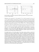
The figure 21 illustrates the advantage of our method to detect changes for real world FDI
applications. Measurements of the stripper level (figure 21 a) are decomposed into 3
components by using filters bank derived from the 'Haar' wavelet packet. From time t
r
= 600
hours, the perturbation IDV16, that corresponds to a random variation of the A, B, C
composition, modifies the dynamical behavior of the system. The detection functions
applied on the 3 components (figure 21 f, g, h) can be compared with the detection function

applied directly on measurement of pressure (figure 21 b). After fusion, the point of change
is calculated to be t
f
= 659. Detection results are considerably improved by using the derived
filters bank as a preprocessor.

Fig. 21. Analysis of the stripper level measurements (%) for TECP with robust adaptive
control and for IDV 16 perturbation from t = 600.
At left: decomposition of the signal into 3 components.
At right: the detection functions of each component.
a) Original signal b) DCS applied directly on the original signal.
c) d) e) Decomposition using filters bank derived from the 'Haar' wavelet packet.
f) g) h) Detection functions applied on the filtered signals (c, d, e).
6. Conclusions and perspectives
The aim of our work is to detect the point of change of statistical parameters in signals
collected from complex industrial systems. This method uses a filters bank derived from a
wavelet packet and combined with DCS to characterize and classify the parameters of a
signal in order to detect any variation of the statistical parameters due to any change in
frequency and energy. The main contribution of this paper is to derive the parameters of a
filters bank that behaves as a wavelet packet. The proposed algorithm provides also good
results for the detection of frequency changes in the signal. The application to the Tennessee
Eastman Challenge Process illustrates the interest of the approach for on–line detection and
real world applications.
Fault Detection Algorithm Based on Filters Bank Derived from Wavelet Packets

203
In the future, our algorithm will be tested with more data issued form several systems in
order to improve and validate it and to compare it to other methods. We will consider
mechanical and electrical machines (Awadallah & Morcos 2003, Benbouzid et al.,1999), and
as a consequence our intend is to develop FDI methods for wind turbines and renewable

multi-source energy systems (Guérin et al., 2005).
7. References
Awadallah M., M.M. Morcos, Application of AI tools in faults diagnosis of electrical
machines and drives – a review, Trans. IEEE Energy Conversion, vol. 18, no. 2, pp.
245-251, june 2003.
Basseville M., Nikiforov I. Detection of Abrupt Changes: Theory and Application. Prentice-
Hall, Englewood Cliffs, NJ, 1993.
Benbouzid M., M. Vieira, C. Theys, "Induction motor's faults detection and localization
using stator current advanced signal processing techniques", IEEE Transaction on
Power Electronics, Vol. 14, N° 1, pp 14 – 22, January1999.
Blanke M., Kinnaert M., Lunze J., Staroswiecki M., Diagnosis and fault tolerant control,
Springer Verlag, New York, 2003.
Coifman R. R., and Wicherhauser M.V. (1992): ‘Entropy based algorithms for best basis selection’,
IEEE Trans. Inform. Theory, 38, pp. 713-718.
Downs, J.J., Vogel, E.F, 1993, A plant-wide industrial control problem, Computers and
Chemical Engineering, 17, pp. 245-255.
Flandrin P. Temps fréquence, édition HERMES, Paris,1993.
Guérin F., Druaux F., Lefebvre D., Reliability analysis and FDI methods for wind turbines: a
state of the art and some perspectives, 3ème French - German Scientific conference
« Renewable and Alternative Energies», December 2005, Le Havre and Fécamp,
France.
Hitti. Eric 3 Sélection d'un banc optimal de filtres à partir d'une décomposition en paquets
d'ondelettes. Application à la détection de sauts de fréquences dans des signaux
multicomposantes » THESE de DOCTORAT, Sciences de l'Ingénieur, Spécialité:
Automatique et Informatique Appliquee, 9 novembre 1999, Ecole Centrale de
Nantes.
Khalil.M, Une approche pour la détection fondée sur une somme cumulée dynamique
associée à une décomposition multiéchelle. Application à l'EMG utérin. Dix-
septième Colloque GRETSI sur le traitement du signal et des images, Vannes,
France,1999.

Khalil M., Duchêne J., Dynamic Cumulative Sum approach for change detection, EDICS NO:
SP 3.7. 1999.
Leclercq, E., Druaux, F. Lefebvre, D., Zerkaoui, S., 2005. Autonomous learning algorithm for
fully connected recurrent networks. Neurocomputing, vol. 63, pp. 25-44.
Mallat S. (1999): ‘A Wavelet Tour of Signal Processing’, Academic Press, San Diego, CA.
Mallat S. Une exploration des signaux en ondelettes, les éditions de l’école
polytechnique, Paris, juillet 2000. http ://www.cmap.polytechnique.fr/~mallat/
Wavetour_fig/.
Chendeb Marwa, Détection et caractérisation dans les signaux médicaux de longue durée par la
théorie des ondelettes. Application en ergonomie, stage du DEA modélisation et
simulation informatique (AUF), octobre 2002.
Robotics, Automation and Control

204
Maquin D. and Ragot J., Diagnostic des systèmes linéaires, Hermes, Paris, 2000.
Mustapha O., Khalil M., Hoblos G, Chafouk H., Ziadeh H., Lefebvre D., About the
Detectability of DCS Algorithm Combined with Filters Bank, Qualita 2007, Tanger,
Maroc, April 2007.
Mustapha O, Khalil M., Hoblos G, Chafouk H., Lefebvre D., Fault detection algorithm using
DCS method combined with filters bank derived from the wavelet transform, IEEE – IFAC
ICINCO 2007, 09- 11 May, Angers, France, 2007.
Nikiforov I. Sequential detection of changes in stochastic systems. Lecture notes in Control and
information Sciences, NY, USA, 1986, pp. 216-228.
Papalambros P. Y, Wilde J. D. Principles of optimal design. Modeling and computation.
Cambridge university press, USA, 2000.
Patton R.J., Frank P.M. and Clarck R., Issue of Fault diagnosis for dynamic systems, Springer
Verlag, 2000.
Rardin L. R. Optimization in operation research. Prentice-Hall, NJ, USA, 1998.
Rustagi S. J. Optimization techniques in statistics. Academic press, USA, 1994.
Saporta G. Probabilités, analyse des données et statistiques, éditions Technip, 1990.

Singhal, A., 2000. Tennessee Eastman Plant Simulation with Base Control System of
McAvoy and Ye., Research report, Department of Chemical Engineering, University
of California, Santa Barbara, USA.
Zerkaoui S., Druaux F., Leclercq E., Lefebvre D., 2007, Multivariable adaptive control for non-
linear systems : application to the Tennessee Eastman Challenge Process, ECC 2007, Kos,
Greece, July 2 – 5.
Zwingelstein G., Diagnostic des défaillances, Hermes, Paris, 1995.
12
Pareto Optimum Design of Robust Controllers
for Systems with Parametric Uncertainties
Amir Hajiloo
1
, Nader Nariman-zadeh
1 2
and Ali Moeini
3
,

1
Dept. of Mechanical Engineering, Faculty of Engineering, University of Guilan
2
Intelligent-based Experimental Mechanics Center of Excellence, School of Mechanical
Engineering, Faculty of Engineering, University of Tehran
3
Dept. of Algorithms & Computations, Faculty of Engineering, University of Tehran
Iran
1. Introduction
The development of high-performance controllers for various complex problems has been a
major research activity among the control engineering practitioners in recent years. In this
way, synthesis of control policies have been regarded as optimization problems of certain

performance measures of the controlled systems. A very effective means of solving such
optimum controller design problems is genetic algorithms (GAs) and other evolutionary
algorithms (EAs) (Porter & Jones, 1992; Goldberg, 1989). The robustness and global
characteristics of such evolutionary methods have been the main reasons for their extensive
applications in off-line optimum control system design. Such applications involve the
design procedure for obtaining controller parameters and/or controller structures. In
addition, the combination of EAs or GAs with fuzzy or neural controllers has been reported
in literature which, in turn, constitutionally formed intelligent control scheme (Porter et al.,
1994; Porter & Nariman-zadeh, 1995; Porter & Nariman-zadeh, 1997). The robustness and
global characteristics of such evolutionary methods have been the main reasons for their
extensive applications in off-line optimum control system design. Such applications involve
the design procedure for obtaining controller parameters and/or controller structures. In
addition to the most applications of EAs in the design of controllers for certain systems,
there are also much research efforts in robust design of controllers for uncertain systems in
which both structured or unstructured uncertainties may exist (Wolovich, 1994). Most of the
robust design methods such as μ-analysis, H
2
or H
∞
design are based on different norm-
bounded uncertainty (Crespo, 2003). As each norm has its particular features addressing
different types of performance objectives, it may not be possible to achieve all the robustness
issues and loop performance goals simultaneously. In fact, the difficult mixed norm-control
methodology such as H
2
/ H
∞
has been proposed to alleviate some of the issue of meeting
different robustness objectives (Baeyens & Khargonekar, 1994). However, these are based on
the worst case scenario considering in the most possible pessimistic value of the

performance for a particular member of the set of uncertain models (Savkin et al., 2000).
Consequently, the performance characteristics of such norm-bounded uncertainties robust
designs often degrades for the most likely cases of uncertain models as the likelihood of the
Robotics, Automation and Control

206
worst-case design is unknown in practice (Smith et al., 2005). Recently, there have been
many efforts for designing robust control methods. In these methods for reducing the
conservatism or accounting more for the most likely plants with respect to uncertainties, the
probabilistic uncertainty, as a weighting factor, propagates through the uncertain parameter
of plants. In fact, probabilistic uncertainty specifies set of plants as the actual dynamic
system to each of which a probability density function (PDF) is assigned (Crespo & Kenny,
2005). Therefore, such additional information regarding the likelihood of each plant allows a
reliability-based design in which probability is incorporated in the robust design. In this
method, robustness and performance are stochastic variables (Stengel & Ryan, 1989).
Stochastic behavior of the system can be simulated by Monte- Carlo Simulation (Ray &
Stengel, 1993). Robustness and performance can be considered as objective functions with
respect to the controller parameters in optimization problem. GAs have also been recently
deployed in an augmented scalar single objective optimization to minimize the probabilities
of unsatisfactory stability and performance estimated by Monte Carlo simulation (Wang &
Stengel, 2001), (Wang & Stengel, 2002). Since conflictions exist between robustness and
performance metrics, choosing appropriate weighting factor in a cost function consisting of
weighted quadratic sum of those non-commensurable objectives is inherently difficult and
could be regarded as a subjective design concept. Moreover, trade-offs existed between
some objectives cannot be derived and it would be, therefore, impossible to choose an
appropriate optimum design reflecting the compromise of the designer’s choice concerning
the absolute values of objective functions. Therefore, this problem can be formulated as a
multi objective optimization problem (MOP) so that trade-offs between objectives can be
derived consequently.
In this chapter, a new simple algorithm in conjunction with the original Pareto ranking of

non-dominated optimal solutions is first presented for MOPs in control systems design. In
this Multi-objective Uniform-diversity Genetic Algorithm (MUGA), a є-elimination diversity
approach is used such that all the clones and/or є-similar individuals based on normalized
Euclidean norm of two vectors are recognized and simply eliminated from the current
population. Such multi-objective Pareto genetic algorithm is then used in conjunction with
Monte-Carlo simulation to obtain Pareto frontiers of various non-commensurable objective
functions in the design of robust controllers for uncertain systems subject to probabilistic
variations of model parameters. The methodology presented in this chapter simply allows
the use of different non-commensurable objective functions both in frequency and time
domains. The obtained results demonstrate that compromise can be readily accomplished
using graphical representations of the achieved trade-offs among the conflicting objectives.
2. Stochastic robust analysis
In real control engineering practice, there exist a variety of typical sources of uncertainty
which have to be compensated through robust control design approach. Those uncertainties
include plant parameter variations due to environmental condition, incomplete knowledge
of the parameters, age, un-modelled high frequency dynamics, and etc. Two categorical
types of uncertainty, namely, structured uncertainty and unstructured uncertainty are
generally used in classification. The structured uncertainty concerns about the model
uncertainty due to unknown values of parameters in a known structure. In conventional
optimum control system design, uncertainties are not addressed and the optimization
process is accomplished deterministically. In fact, it has been shown that optimization
Pareto Optimum Design of Robust Controllers for Systems with Parametric Uncertainties

207
without considering uncertainty generally leads to non-optimal and potentially high risk
solution (Lim et al., 2005). Therefore, it is very desirable to find robust design whose
performance variation in the presence of uncertainties is not high. Generally, there exist two
approaches addressing the stochastic robustness issue, namely, robust design optimization
(RDO) and reliability-based design optimization (RBDO) (Papadrakakis et al., 2004). Both
approaches represent non deterministic optimization formulations in which the probabilistic

uncertainty is incorporated into the stochastic optimal design process. Therefore, the
propagation of a priori knowledge regarding the uncertain parameters through the system
provides some probabilistic metrics such as random variables (e.g., settling time, maximum
overshoot, closed loop poles, …), and random processes (e.g., step response, Bode or
Nyquist diagram, …) in a control system design (Smith et al., 2005). In RDO approach, the
stochastic performance is required to be less sensitive to the random variation induced by
uncertain parameters so that the performance degradation from ideal deterministic
behaviour is minimized. In RBDO approach, some evaluated reliability metrics subjected to
probabilistic constraints are satisfied so that the violation of design requirements is
minimized. In this case, limit state functions are required to define the failure of the control
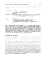
system. Figure (1) depicts the concept of these two design approaches where f is to be
minimized. Regardless the choice of any of these two approaches, random variables and
random processes should be evaluated reflecting the effect of probabilistic nature of
uncertain parameters in the performance of the control system.


Fig. 1. Concepts of RDO and RBDO optimization
With the aid of ever increasing computational power, there have been a great amount of
research activities in the field of robust analysis and design devoted to the use of Monte
Carlo simulation (Crespo, 2003; Crespo & Kenny, 2005; Stengel, 1986; Stengel & Ryan, 1993;
Papadrakakis et al., 2004; Kang, 2005). In fact, Monte Carlo simulation (MCS) has also been
used to verify the results of other methods in RDO or RBDO problems when sufficient
number of sampling is adopted (Wang & Stengel, 2001). Monte Carlo simulation (MCS) is a
direct and simple numerical method but can be computationally expensive. In this method,
random samples are generated assuming pre-defined probabilistic distributions for
Robotics, Automation and Control

208
uncertain parameters. The system is then simulated with each of these randomly generated
samples and the percentage of cases produced in failure region defined by a limit state

function approximately reflects the probability of failure.
Let X be a random variable, then the prevailing model for uncertainties in stochastic
randomness is the probability density function (PDF),
(
)
xf
X
or equivalently by the
cumulative distribution function (CDF),
(
)
xF
X
, where the subscript X refers to the random
variable. This can be given by

() ( ) ()
Pr
x
XX
F
xXxfxdx
−∞
=≤=
∫
(1)
where Pr(.) is the probability that an event (X≤x) will occur. Some statistical moments such
as the first and the second moment, generally known as mean value (also referred to as
expected value) denoted by E(X) and variance denoted by
()

X
2
σ
, respectively, are the most
important ones. They can also be computed by

() () ()
XX
EX xdF x f xdx
∞∞
−∞ −∞
==
∫∫
(2)
and

() ()()()
∫
∞
∞−
−= dxxfXExX
X
2
σ
(3)
In the case of discrete sampling, these equations can be readily represented as
()
∑
=
≅

N
i
i
x
N
XE
1
1

(4)
and
() ()
()
∑
=
−
−
≅
N
i
i
XEx
N
X
1
2
2
1
1
σ

(5)
where
i
x
is the i
th
sample and N is the total number of samples.
In the reliability-based design, it is required to define reliability-based metrics via some
inequality constraints (in time or frequency domain). Therefore, in the presence of uncertain
parameters of plant (p) whose PDF or CDF can be given by f
p
(p) or F
p
(p), respectively, the
reliability requirements can be given as

(
)
(
)
Pr p 0 1, 2, ,
i
fi
P
gik
ε
=≤≤=
(6)
In equation (6),

i
f
P
denotes the probability of failure (i.e.,
(
)
0≤p
i
g
) of the i
th
reliability
measure and k is the number of inequality constraints (i.e., limit state functions) and is the
highest value of desired admissible probability of failure. It is clear that the desirable value
of each
i
f
P
is zero. Therefore, taking into consideration the stochastic distribution of
Pareto Optimum Design of Robust Controllers for Systems with Parametric Uncertainties

209
uncertain parameters ( p ) as
(
)
p
p
f
, equation (6) can now be evaluated for each probability
function as

()
()
()
()
∫
≤
=≤=
0
0Pr
p
p
ppp
i
g
i
i
f
dfgP

(7)
This integral is, in fact, very complicated particularly for systems with complex g(p) (Wang
& Stengel, 2002) and Monte Carlo simulation is alternatively used to approximate equation
(7). In this case, a binary indicator function
I
g(p)
is defined such that it has the value of 1 in
the case of failure (g(p)≤0) and the value of zero otherwise,
()
(
)

()
⎩
⎨
⎧
≤
>
=
01
00
p
p
p
g
g
I
g

(8)
Consequently, for each limit state function, g(p), the integral of equation (7) can be rewritten as
()
()
()
()
()()
∫
∞
∞−
= ppkpp
pp
dfCGIP

gf
,

(9)
where G(p) is the uncertain plant model and C(k) is the controller to be designed in the case
of control system design problems. Based on Monte Carlo simulation (Ray & Stengel, 1993;
Wang & Stengel, 2001; Wang & Stengel, 2002; Kalos, 1986), the probability using sampling
technique can be estimated using
()
()
()
()
()
∑
=
=
N
i
gf
CGI
N
P
i
1
,
1
kpp
p

(10)

where G
i
is the i
th
plant that is simulated by Monte Carlo Simulation. In other words, the
probability of failure is equal to the number of samples in the failure region divided by the
total number of samples. Evidently, such estimation of P
f
approaches to the actual value in
the limit as
∞
→N (Wang & Stengel, 2002). However, there have been many research
activities on sampling techniques to reduce the number of samples keeping a high level of
accuracy. Alternatively, the quasi-MCS has now been increasingly accepted as a better
sampling technique which is also known as Hammersley Sequence Sampling (HSS) (Smith
et al., 2005; Crespo & Kenny, 2005). In this paper, HSS has been used to generate samples for
probability estimation of failures. In a RBDO problem, the probability of representing the
reliability-based metrics given by equation (10) is minimized using an optimization method.
In a multi-objective optimization of a RBDO problem presented in this paper, however,
there are different conflicting reliability-based metrics that should be minimized
simultaneously.
In the multi-objective RBDO of control system problems, such reliability-based metrics
(objective functions) can be selected as closed-loop system stability, step response in time
domain or Bode magnitude in frequency domain, etc. In the probabilistic approach, it is,
therefore, desired to minimize both the probability of instability and probability of failure to
a desired time or frequency response, respectively, subjected to assumed probability
Robotics, Automation and Control

210
distribution of uncertain parameters. In a RDO approach that is used in this work, the lower

bound of degree of stability that is the distance from critical point -1 to the nearest point on
the open lop Nyquist diagram, is maximized. The goal of this approach is to maximize the
mean of the random variable (degree of stability) and to minimize its variance. This is in
accordance with the fact that in the robust design the mean should be maximized and its
variability should be minimized simultaneously (Kang, 2005). Figure (2) depicts the concept
of this RDO approach where
(
)
xf
X
is a PDF of random variable, X. It is clear from figure (2)
that if the lower bound of
X is maximized, a robust optimum design can be obtained.
Recently, a weighted-sum multi-objective approach has been applied to aggregate these
objectives into a scalar single-objective optimization problem (Wang & Stengel, 2002; Kang,
2005).


Fig. 2. Concept of RDO approach
However, the trade-offs among the objectives are not revealed unless a Pareto approach of
the multi-objective optimization is applied. In the next section, a multi-objective Pareto
genetic algorithm with a new diversity preserving mechanism recently reported by some of
authors (Nariman-Zadeh et al., 2005; Atashkari et al., 2005) is briefly discussed for a
combined robust and reliability-based design optimization of a control system.
3. Multi-objective Pareto optimization
Multi-objective optimization which is also called multi-criteria optimization or vector
optimization has been defined as finding a vector of decision variables satisfying constraints
to give optimal values to all objective functions (Atashkari et al., 2005; Coello Coello &
Christiansen, 2000; Coello Coello et al., 2002; Pareto, 1896). In general, it can be
mathematically defined as follows; find the vector

[
]
T
n
xxxX
**
2
*
1
*
, ,,=
to optimize

[
]
T
k
XfXfXfXF )(), ,(),()(
21
=
(11)
Pareto Optimum Design of Robust Controllers for Systems with Parametric Uncertainties

211
subject to m inequality constraints

(
)
miXg
i

10
=
≤
(12)
and
p equality constraints

(
)
pjXhj 10
=
≤
(13)
where,
n
X ℜ∈
*
is the vector of decision or design variables, and
k
XF ℜ∈)(
is the vector of
objective functions. Without loss of generality, it is assumed that all objective functions are
to be minimized. Such multi-objective minimization based on the Pareto approach can be
conducted using some definitions.
Pareto dominance
A vector
[]
k
k
uuu ℜ∈= , ,,

21
U
dominates to vector
[
]
k
k
vvv ℜ∈= , ,,
21
V
(denoted by
VU ≺ ) if and only if
}
{
}
{
jjii
vukjvuki
<
∈
∃
∧
≤
∈
∀
:, ,2,1,, ,2,1
. It means that there is at
least one
u
j

which is smaller than v
j
whilst the rest u’s are either smaller or equal to
corresponding
v’s.
Pareto optimality
A point
Ω∈
*
X
(
Ω
is a feasible region in
n
ℜ ) is said to be Pareto optimal (minimal) with
respect to all
Ω
∈
X
if and only if
)()(
*
XFXF ≺
. Alternatively, it can be readily restated as
}{
ki , ,2,1∈∀
,
},{
*
XX −Ω∈∀

)()(
*
XfXf
ii
≤
∧
}
{
kj , ,2,1
∈
∃
:
)()(
*
XfXf
jj
<
. It means that
the solution
X
*
is said to be Pareto optimal (minimal) if no other solution can be found to
dominate X
*
using the definition of Pareto dominance.
Pareto Set
For a given MOP, a Pareto set Ƥ٭ is a set in the decision variable space consisting of all the
Pareto optimal vectors, Ƥ٭
|{
Ω

∈
=
X
∄
)}()(: XFXFX ≺
′
Ω
∈
′
. In other words, there is no
other
X’ in that dominates any
∈
X
Ƥ٭
Pareto front
For a given MOP, the Pareto front ƤŦ٭ is a set of vectors of objective functions which are
obtained using the vectors of decision variables in the Pareto set Ƥ٭, that is,
ƤŦ٭
∈== XX
k
fXfXfXF :))( ,),(
2
),(
1
()({
Ƥ٭}. Therefore, the Pareto front ƤŦ٭ is a set of
the vectors of objective functions mapped from Ƥ٭.
Evolutionary algorithms have been widely used for multi-objective optimization because of
their natural properties suited for these types of problems. This is mostly because of their

parallel or population-based search approach. Therefore, most difficulties and deficiencies
within the classical methods in solving multi-objective optimization problems are
eliminated. For example, there is no need for either several runs to find the Pareto front or
quantification of the importance of each objective using numerical weights. It is very
important in evolutionary algorithms that the genetic diversity within the population be
preserved sufficiently (Osyezka, 1985). This main issue in MOPs has been addressed by
Robotics, Automation and Control

212
much related research work (Nariman-zadeh et al., 2005; Atashkari et al., 2005; Coello
Coello & Christiansen, 2000; Coello Coello et al., 2002; Pareto, 1896; Osyezka, 1985; Toffolo &
Benini, 2002; Deb et al., 2002; Coello Coello & Becerra, 2003; Nariman-zadeh et al., 2005).
Consequently, the premature convergence of MOEAs is prevented and the solutions are
directed and distributed along the true Pareto front if such genetic diversity is well
provided. The Pareto-based approach of NSGA-II (Osyezka, 1985) has been recently used in
a wide range of engineering MOPs because of its simple yet efficient non-dominance
ranking procedure in yielding different levels of Pareto frontiers. However, the crowding
approach in such a state-of-the-art MOEA (Coello Coello & Becerra, 2003) works efficiently
for two-objective optimization problems as a diversity-preserving operator which is not the
case for problems with more than two objective functions. The reason is that the sorting
procedure of individuals based on each objective in this algorithm will cause different
enclosing hyper-boxes. It must be noted that, in a two-objective Pareto optimization, if the
solutions of a Pareto front are sorted in a decreasing order of importance to one objective,
these solutions are then automatically ordered in an increasing order of importance to the
second objective. Thus, the hyper-boxes surrounding an individual solution remain
unchanged in the objective-wise sorting procedure of the crowding distance of NSGA-II in
the two-objective Pareto optimization problem. However, in multi-objective Pareto
optimization problem with more than two objectives, such sorting procedure of individuals
based on each objective in this algorithm will cause different enclosing hyper boxes. Thus,
the overall crowding distance of an individual computed in this way may not exactly reflect

the true measure of diversity or crowding property for the multi-objective Pareto
optimization problems with more than two objectives.
In our work, a new method is presented to modify NSGA-II so that it can be safely used for
any number of objective functions (particularly for more than two objectives) in MOPs. Such
a modified MOEA is then used for multi-objective robust desing of linear controllers for
systems with parametric uncertainties.

4. Multi-objective Uniform-diversity Genetic Algorithm (MUGA)


The multi-objective uniform-diversity genetic algorithm (MUGA) uses non-dominated
sorting mechanism together with a ε-elimination diversity preserving algorithm to get
Pareto optimal solutions of MOPs more precisely and uniformly (Jamali et.al., 2008.)
4.1 The non-dominated sorting method

The basic idea of sorting of non-dominated solutions originally proposed by Goldberg
(Goldberg, 1989) used in different evolutionary multi-objective optimization algorithms
such as in NSGA-II by Deb (Deb et al., 2002) has been adopted here. The algorithm simply
compares each individual in the population with others to determine its non-dominancy.
Once the first front has been found, all its non-dominated individuals are removed from the
main population and the procedure is repeated for the subsequent fronts until the entire
population is sorted and non-dominately divided into different fronts.
A sorting procedure to constitute a front could be simply accomplished by comparing all the
individuals of the population and including the non-dominated individuals in the front.
Such procedure can be simply represented as following steps:

Pareto Optimum Design of Robust Controllers for Systems with Parametric Uncertainties

213

1-Get the population (pop)
2-Include the first individual {ind(1)} in the front P* as P*(1), let P*_size=1;
3-Compare other individuals {ind (j), j=2, Pop_size)} of the pop with { P*(K), K=1, P*_size}
of the P*;
If ind(j)<P*(K) replace the P*(K) with ind(j)
If P*(K)<ind(K), j=j+1, continue comparison;
Else include ind(j) in P*, P*_size= P*_size+1, j=j+1, continue comparison;
4-End of front P*;

It can be easily seen that the number of non-dominated solutions in P* grows until no further
one is found. At this stage, all the non-dominated individuals so far found in
P* are removed
from the main population and the whole procedure of finding another front may be
accomplished again. This procedure is repeated until the whole population is divided into
different ranked fronts. It should be noted that the first rank front of the final generation
constitute the final Pareto optimal solution of the multi-objective optimization problem.
4.2 The ε-elimination diversity preserving approach
In the ε-elimination diversity approach that is used to replaced the crowding distance
assignment approach in NSGA-II (Deb et al., 2002), all the clones and ε-similar individuals
are recognized and simply eliminated from the current population. Therefore, based on a
value of ε as the elimination threshold, all the individuals in a front within this limit of a
particular individual are eliminated. It should be noted that such ε-similarity must exist both
in the space of objectives and in the space of the associated design variables. This will ensure
that very different individuals in the space of design variables having ε-similarity in the
space of objectives will not be eliminated from the population. The pseudo-code of the ε-
elimination approach is depicted in figure (3). Evidently, the clones and ε-similar


Fig. 3. The ε-elimination diversity preserving pseudo-code
ε-elim= ε-elimination(pop) // pop includes design variables and

objective function
i=1; j=1;
get K (K=1 for the first front);
While i,j <pop_size
e(i,j)= ║X(i,:),X(j,:) ║/║X(i,:) ║; X(i),X(j)
∈
P*
k
Ụ PF*
k
//finding mean value of ε
within pop.
end
ε=mean(e);
i=1;
until i+1<pop_size;
j=i+1
until j<pop_size
if e(i,j)<ε
then {pop}={pop}/ {pop(j)} //remove the ε-similar individual
j=j+1
end
i=i+1
end
Robotics, Automation and Control

214
individuals are replaced from the population by the same number of new randomly
generated individuals. Meanwhile, this will additionally help to explore the search space of
the given MOP more effectively. It is clear that such replacement does not appear when a

front rather than the entire population is truncated for ε-similar individual.
4.3 The main algorithm of MUGA
It is now possible to present the main algorithm of MUGA which uses both non-dominated
sorting procedure and ε-elimination diversity preserving approach and is given in figure (4).


Fig. 4. The pseudo-code of the main algorithm of MUGA
It first initiates a population randomly. Using genetic operators, another same size
population is then created. Based on the ε-elimination algorithm, the whole population is
then reduced by removing ε-similar individuals. At this stage, the population is re-filled by
randomly generated individuals which helps to explore the search space more effectively.
The whole population is then sorted using non-dominated sorting procedure. The obtained
fronts are then used to constitute the main population. It must be noted that the front which
must be truncated to match the size of the population is also evaluated by ε-elimination
procedure to identify the ε-similar individuals. Such procedure is only performed to match
Get N //population size
t=1 ; //set generation number
Random_N(P
t
); //generate the first population (P
1
) randomly
Q
t
=Recomb(P
t
) //generate population Q
t
from P
t

by genetic operators
R
t
=P
t
Ụ Q
t
//union of both parent and offspring population
R
t
′=ε-elimination (R
t
) //remove ε-similar individuals in R
t

R
t
′′= R
t
′ Ụ Random_(R
t_
size-R′
t_
size) (P
t
′) //add random individuals to fill R
t
to 2N

Do non-dominate sorting procedure (R

t
′′) //R
t
′′=P*
1
Ụ P*
2
Ụ…ỤP*
k
where k is total
number of fronts
i=1
P
t+1
=Θ
While not P
t+1_
size>N //includes fronts into new population
P
t+1
= P
t+1
Ụ P*
i

i=i+1
end
N′=N- P
t+1_
size

While not (0.9 N′< P
t+1_
size<1.1 N′) //remove the ε-similar individuals within
the tolerance of ±10 percent
Ғ′=ε-elimination (P*
i-1
)
If Ғ′_size< N′
e=1.1*e
else
e=0.9 * e //adjust the value of threshold to get the right population
size of the last front
end
end
t=t+1 //Start next generation

Pareto Optimum Design of Robust Controllers for Systems with Parametric Uncertainties

215
the size of population within ±10 present deviation to prevent excessive computational
effort to population size adjustment. Finally, unless the number of individuals in the first
rank front is changing in certain number of generations, randomly created individuals are
inserted in the main population occasionally (e.g. every 20 generations of having non-
varying first rank front).
5. Process model and controller evaluation method
In this section, the process models and the robust PI/PID controller design methodologies
are presented using some conflicting objective functions defined in both time and frequency
domains.
5.1 The process model
Many industrial systems can be adequately presented by a first-order lag with time delay

(Toscana, 2005) as
()
Ts
ke
sG
s
+
=
−
1
τ

(14)
In the case of stochastic robust design, parameters of the plant given by equation (14) vary
according to
a priori known probabilistic distribution functions around a nominal set of
parameters. In this work, beta distributions with the coefficients of 2 and 2 with the limits of
%50± of the nominal values of plant parameters, 1
=
=
=
Tk
τ
have been selected,
respectively. Stochastic step response of the 10 samples that are simulated by Monte Carlo
simulation is shown in figure (5). It is clear from figure (5) that the response of the uncertain
system has a large variability and the performance of the system deteriorates significantly
with parameters variation. Consequently, the controller design must be accomplished
robustly.

Fig. 5. Stochastic step response of the uncertain plant
Robotics, Automation and Control

216
5.2 The robust design of PI/PID controllers
Simple structure PI/PID Controllers are widely used for many industrial processes
represented by the transfer function of equation (14). The transfer functions,
C(s), of the
standard PI/PID Controllers of the feedback control system shown in figure (6) are
()
()
⎪
⎩
⎪
⎨
⎧
++=
+=
sK
s
K
KsC
s
K
KsC
d
i
p
i

p

(15)

Fig. 6. Closed loop SISO system with plant G(s) and controller C(s)
The design vector of the PI and PID controllers are k
PI
= [K
p
,
K
i
] and k
PID
= [K
p
,
K
i
,
K
d
],
respectively. They have to be optimally determined based on the mixed robust and
reliability-based multi-objective Pareto approach for the uncertain first-order system using
some stochastic evaluation metrics that are introduced as follows.
Two robust performance metrics have been proposed in this work, performance metrics in
time domain and performance metrics in frequency domain. In this section, design vector of
PI controller is obtained based on time domain performance metrics and design vector of
PID controller is obtained based on frequency domain performance metrics.

The most important goal of robust controller design is the robust stability which implies that
all the closed-loop poles of the system remain in the stable left half-plane (
()
0<
ℜ
i
s
) in the
presence of any uncertainty in the nominal plant’s transfer function. Thus, in the case of
stochastic robust design, the limit state function to define the probability of failure of robust
stability will be represented by

(
)
(
)
(
)
(
)
{
}
Nisssg
i
n
ii
ins
,,2,1,,,max
21
… =ℜℜℜ−=p

(16)
where, g
ins
(p) is the limit state function of the instability,
(
)
i
sℜ
is the real part of the closed-
loop poles of the i
th
uncertain plants, and n is the order of the closed-loop plant.
The probability of failure of stochastic stability can now be computed using by equation (10)
()
()
()
∑
=
=
N
i
igins
CGI
N
ins
1
,
1
Pr kp

(17)
in association with equation (16) employing the quasi Monte Carlo Sampling or HSS for N
samples. For obtaining the acceptable stability, such probability of instability should be
minimized.
In addition to the minimizing the probability of instability, maximizing the stability margin
in the frequency domain is another important measure of good performance of a robust
Pareto Optimum Design of Robust Controllers for Systems with Parametric Uncertainties

217
controller for uncertain systems. The inclusion of the stability margin (to be maximized) in
the vector of the cost functions ensures that stable PI/PID controllers having the most
stability margin are obtained. Such robust stability margin, also referred to as degree of
stability
1−
∞
S
, can be simply computed using the sensitivity transfer function
)(1
1
)()(1
1
)(
sLsGsC
sS
+
=
+
=
(18)
for a unity feedback control system shown in figure (6). In frequency domain, the return

difference
(
)
(
)
ωω
jLjL +=−− 11
simply represents the length of a vector drawn from
critical point -1 to open-loop transfer function in the Nyquist diagram. Consequently, the
inverse of ∞-norm of sensitivity transfer function given by equation (18)
(
)
ω
ω
jLSS +==
−
∞
−
∞
1min
1
1

(19)
represents the minimum distance of the Nyquist diagram to point -1. In the case of
stochastic robust design, the degree of stability for each stochastic system is a random
variable. Therefore, in a RDO problem considered in this study the lower bound of
interested random variable (degree of stability) is maximized using an optimization method.
It should be noted that the degree of stability given by equation (19) also directly represents
the additive disturbance rejection property as follows

)()()()(
)(1
)(
)( sDsSsGsD
sL
sG
sY =
+
=
(20)
where, D(s) is the load disturbance transfer function. It is evident from equation (20) that
maximizing the minimum value of
(
)
ω
jL+1
based on equation (19) will cause a better
disturbance rejection according to equation (20). Therefore, systems with high degree of
stability represent a good ability to reject the load disturbance (Toscana, 2005).
A good step response behavior of the system is one of the performance metrics in controller
design procedure that illustrates how system acts in transient and steady state periods.
Another method to obtain these properties of the step response is Bode magnitude of the
close-loop or complementary transfer function. In the stochastic robust design both step
response and Bode magnitude are random process.
In the reliability- based design approach, it is desired to minimize the probability of a failure
of a random process as a function of
w (w represents time or frequency) due to the uncertain
probabilistic parameters. In this approach, let h(p,w) is the random response (step response
or Bode magnitude) of an uncertain plant due to uncertain parameters p, and let define
()

wh and
()
wh
as upper and lower failure boundary, respectively. Therefore, if the random
process is held within these bounds, the uncertain system has a robust performance.
In this work, step response metrics are used to design PI controller and Bode magnitude
metrics are used to design PID controllers.
The lower and upper failure boundaries to define the corresponding limit state
function,
()
0
≤
p
resp
g
, in time domain is given using the Heaviside function

(
)
(
)
(
)
7H25.03H8.0H1.0
−
+
−
+
−
=

ttth
(21a)

(
)
(
)
7H15.0H2.1 −−= tth
(21b)
Robotics, Automation and Control

218
for a period of
t∈[0, t
f
], t
f
= 15. If
r
and r are defined as
t
i
i
i
kihhr , ,2,1,1
=
<
=

0

=
i
r
otherwise
(22a)
tiii
kihhr , ,2,1,1 =>=

0
=
i
r
otherwise
(22b)
where h is the time response of the plant and k
t
is the number of sample time, the limit state
function indicator can then be computed as
()
(
)
∑
=
+==
t
resp
k
i
i
i

t
g
rr
k
I
1
1
p

(23)
which is used in equation (10) to obtain the probability of failure to the desires time
response boundaries.
The complementary transfer function T(s) can be used to obtain closed-loop system response
which is the transfer function of the reference input
R(s) to the output Y(s) and is given as
() ()
(
)
()
sL
sL
sSsT
+
=−=
1
1

(24)
The quantity
()

ω
jT
represents the magnitude of the closed-loop frequency response. It is
well known that the performance of the closed-loop system response is related to
()
ω
jT
. In
order to select appropriate boundaries for such frequency response behavior, the
relationship between peak value of the closed-loop magnitude response (Nise,
2004),
(
)
ω
ω
jTM
p
max= , and the damping ratio,
ζ
, for a second order system with
nominal parameters is considered here as a reference. Such relations are given by
2
12
1
ζζ
−
=
p
M

(25)
at a frequency of
ω
p
given by
2
21
ζωω
−=
np

(26)
Since
ζ and ω
n
are related to maximum overshoot and settling time of step response, respectively,
for a good transient and steady-state response it is required that
+
≥
ζζ
and
+
≥
nn
ωω
. The
selected values of
+
ζ
and

+
n
ω
in this work are 0.7. In order to achieve a good closed-loop
performance, the complementary transfer function T(s) given by equation (24) is used in
frequency domain using lower and upper failure boundaries to define the corresponding
limit state function
(
)
0
≤
p
resp
g
. If
(
)
ω
jTh ≡
which is a random process having sets of CDFs
varying with frequency (Crespo & Kenny, 2005, Crespo, 2003)], both the upper failure
boundary defined by
(
)
ω
h and the lower failure boundary
(
)
ω
h

are used to compute the
probability of failure to a good frequency response. Based on the previous discussion, the
boundaries are defined as
Pareto Optimum Design of Robust Controllers for Systems with Parametric Uncertainties

219
()
[
]
12
10,101
−−
∈=
ωω
h

(27a)
()
[
]
2
10,5.0
7.0
∈=
ω
ω
ω
h

(27b)

If
r
and r are defined as
ω
kihhr
i
i
i
, ,2,1,1
=
<
=

0
=
i
r otherwise
(28a)
ω
kihhr
iii
, ,2,1,1 =>=

0
=
i
r
otherwise
(28b)
where

h is the frequency response of the plant and k
ω
is the number of sample frequency, the
limit state function indicator can then be computed as
()
(
)
∑
=
+==
ω
ω
k
i
i
i
g
rr
k
I
resp
1
1
p

(29)
which is used in equation (10) to obtain the probability of failure to the desired frequency
response boundaries of the complementary transfer function.
6. Results
The objectives Pr

ins
, Pr
resp
and
1−
∞
S
are now considered simultaneously in a Pareto
optimization process to obtain some important trade-offs among the conflicting objectives.
In a mixed robust and reliability-based design approach, the vector of objective functions to
be optimized in a Pareto sense is given as follows

],Pr,[Pr
1−
∞
= SF
respins

(30)
which are computed using equations (17), (23), (29), and (19), respectively, in the quasi-
Monte Carlo simulation process. The evolutionary process of the Pareto multi-objective
optimization is accomplished using MUGA (Jamali, et.al., 2008) where a population size of
45 has been chosen with crossover probability
P
c
and mutation probability P
m
as 0.85 and
0.09, respectively. The optimization process of the robust PI/PID controllers given by
equation (15) is accomplished by 250 Monte Carlo evaluations using HSS distribution for

each candidate control law during the evolutionary process. The vector of objective
functions given by equation (30) is used to obtain non-dominated optimum PI/PID
controllers to represent the trade-offs among the objective functions.
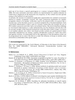
6.1 Pareto optimum PI controllers
A total number of 80 non-dominated optimum design points have been obtained and shown
in figure (7) in the plane of probability of failure to the desired time response (Pr
resp
) and the
degree of stability (). The value of probability of instability (Pr
ins
) of all the non-dominated
optimum points has been obtained zero which demonstrates that all optimum controllers
are stable in the Monte Carlo simulation (Hajiloo et al., 2007).
Robotics, Automation and Control

220

Fig. 7. Pareto fronts of Pr
resp
and degree of stability (
1−
∞
S
)
Since, the value of probability of instability (Pr
ins
) of all non-dominated optimum points has
been found equal to zero, therefore, the result of the 3-objective optimization process
corresponds to a 2-objective optimization process which is shown in figure (7). It can be
observed from the Pareto front of figure (7) that improving one objective will cause another

objective deteriorates accordingly.
The best point obtained for Pr
resp
is point A which corresponds to the worst value of
1−
∞
S
.
These values for time response and degree of stability are 0.0338 and 0.3577, respectively. In
other words, optimum design point A represents 3.38% probability of failure to the desired
time response and its minimum distance to the critical point -1+0j in the Nyquist diagram is
0.3577, representing its degree of stability for 250 Monte Carlo evaluations. Alternatively,
the best value of obtained
1−
∞
S
is that of point C which corresponds to the worst value of
Pr
resp
and are 0.8 and 0.8923, respectively. Figure (8) shows the corresponding 1, 10, 30, 50,
70, 90, 99 percentiles of time responses of both design points A and C which demonstrates
the stochastic behavior of the corresponding PI controllers for 250 Monte Carlo simulations
of the plant subjected to the assumed probabilistic uncertainties. An
m percentiles curve
presents a confidence limit of
m percent probability that the time response behavior would
be below that curve.
By careful investigation of figure (7) an important trade-off can be observed from the Pareto
front of objectives Pr
resp

and
1−
∞
S
. It is clear that the gradient of the Pareto from in section A-
B increases noticeably in section B-C. Apparently, optimum design point B shows a
significant improvement of degree of stability (
1−
∞
S
) in comparison with that of point A
whilst its probability of failure to the desired time response does not degrades significantly
in section A-B as much as it does in section B-C. Thus, optimum design point B representing
a PI controller with K
p
= 0.3 and K
i
= 0.31 can be optimally chosen from a trade-off point of
view for objectives Pr
resp
and
1−
∞
S
. Figure (9) shows percentiles of stochastic time response
behavior of point B which can be compared to those of optimum design points A and C
shown in figure (8).
Pareto Optimum Design of Robust Controllers for Systems with Parametric Uncertainties

221

(a)

(b)
Fig. 8. Step response behaviors of optimum designs (a) point A (b) point C
Table 1 summarizes the values of those objectives together with the corresponding values of
PI controller gains for three optimum design points A, B, and C shown in figure (7).

Design
points
K
p
K
i
Pr
ins
Pr
resp

1−
∞
S

A 0.516 0.454 0 0.0338 0.3577
B 0.3 0.31 0 0.1500 0.5624
C 0.8 0.892 0 0.8 0.8923
Table 1. Optimum values of objective functions and their gains for the PI controller obtained
from 250 Monte Carlo simulations
The robust stability margins of all optimum points have been shown in figure (10). In this
figure, the cumulative distribution functions (CDF) have been shown for all design points. It

is evident that the optimum design point C exhibits the best stability robustness, because
lower bound of its degree of stability is greater than other design points and variance of the
degree of stability of design point C is very small.
Robotics, Automation and Control

222

Fig. 9. Step response behaviors of optimum design B

Fig. 10. CDFs for robust stability margins of different optimum designs
6.2 Pareto optimum PID controllers
A total number of 31 non-dominated optimum design points have been obtained and shown
in figure(11) in the plane of probability of frequency response failure (Pr
resp
) and the degree
of stability (
1−
∞
S
). The value of probability of instability (Pr
ins
) of all the non-dominated
optimum points has been obtained zero which demonstrates that all obtained optimum
controllers are stable in the Monte Carlo simulation. Therefore, the results of the 3-objective
optimization process correspond to those of a 2-objective optimization process excluding the
probability of instability. It can be observed from the Pareto front of figure (11) that improving
one objective will cause another objective deteriorates accordingly. The best point obtained for
Pr
resp
is point A which corresponds to the worst value of

1−
∞
S
. These values for the probability
of frequency response failure and the degree of stability are 0.089 and 0.4815, respectively. In
other words, optimum design point A represents 8.9% probability of frequency response
failure and its minimum distance to the critical point -1+0j in the Nyquist diagram is 0.4815,
representing its degree of stability in 250 Monte Carlo evaluations. Alternatively, the best
value of obtained
1−
∞
S
is that of point C which corresponds to the worst value of Pr
resp
which
are 0.1381 and 0.9798, respectively. In other words, optimum design point C represents
13.81% probability of frequency response failure while its minimum distance to the critical
point -1+0j in the Nyquist diagram is 0.9788 representing its improved degree of stability.
Pareto Optimum Design of Robust Controllers for Systems with Parametric Uncertainties

223

Fig. 11. Pareto fronts of Pr
resp
and degree of stability (
1−
∞
S
)
Figure (12) shows the corresponding 1, 10, 30, 50, 70, 90, 99 percentiles of step response of a

non-dominated optimum design points B which demonstrate the stochastic behavior of the
corresponding PID controllers in 250 Monte Carlo simulations of the plant subjected to the
assumed probabilistic uncertainties in the plant. Figure (13) shows the Nyquist diagram for
the design point B.

Fig. 12. Probabilistic step response behaviors of optimum design B

Fig. 13. Nyquist diagram of optimum design B
Robotics, Automation and Control

224
The robust stability margins of all optimum points have been also shown in figure (14). In
this figure, the cumulative distribution functions (CDF) have been shown for all design
points.

Fig. 14. CDFs for robust stability margins of different optimum designs
Table 2 summarizes the values of those objectives together with the corresponding values of
PID controller gains for three optimum design points A, B, and C shown in figure (11).

Design
points
K
p
K
i
K
d
Pr
ins
Pr

resp

1−
∞
S

A 0.2132 0.4035 0.0572 0 0.0899 0.4815
B 0.2210 0.3879 0.2185 0 0.1299 0.6084
C 0.0130 0.0129 0.0119 0 0.1381 0.9798
Table 2. Optimum values of objective functions and their gains for the PID controller
obtained from 250 Monte Carlo simulations
7. Conclusion
A multi-objective genetic algorithm with a recently developed diversity preserving
mechanism was used to optimally design PI/PID controllers from a reliability-based point
of view in a probabilistic approach. The objective functions which often conflict with each
other were appropriately defined using some probabilistic metrics in time and frequency
domain. The multi-objective optimization of robust PID controllers led to the discovering
some important trade-offs among those objective functions. The framework of such hybrid
application of multi-objective GAs and Monte Carlo Simulation of this work for the Pareto
optimization of both robust and reliability-based approach using some non-commensurable
stochastic objective functions is very promising and can be generally used in the optimum
design of real-world complex control systems with probabilistic uncertainties
8. References
Atashkari, K.; Nariman-zadeh, N.; Jamali A.& Pilechi A. (2005).Thermodynamic Pareto
optimization of turbojet using multi-objective genetic algorithm,
International
Journal of Thermal Science
, Vol. 44, No. 11, 1061-1071, Elsevier
Baeyens, E. & Khargonekar, P. (1994). Some examples in mixed
∞

HH /
2
Control, Proceeding
of American Control Conference
, pp. 1608-1612, USA
Pareto Optimum Design of Robust Controllers for Systems with Parametric Uncertainties

225
Coello Coello, C. A. & Becerra, R. L. (2003). Evolutionary Multi-objective Optimization using
a Cultural Algorithm, IEEE Swarm Intelligence Systems., pp. 6-13, USA
Coello Coello, C. A., & Christiansen, A. D. (2000). Multiobjective optimization of trusses
using genetic algorithms, Computers & Structures, Vol. 75, 647-660
Coello Coello, C. A.; Van Veldhuizen, D. A. & Lamont, G. B. (2002). Evolutionary
Algorithms for Solving Multi-objective problems,
Kluwer Academic Publishers, New
York
Crespo, L.G. & Kenny, S.P. (2005). Robust Control Deign for systems with probabilistic
Uncertainty, NASA report, March 2005, TP-2005-213531
Crespo, L.G. (2003). Optimal performance, robustness and reliability base designs of systems
with structured uncertainty, Proceeding of American Control Conference, pp. 4219-
4224, USA, Denver, Colorado,
Deb, K.; Agrawal, S.; Pratap, A. & Meyarivan, T. (2002). A fast and elitist multi-objective
genetic algorithm: NSGA-II,
IEEE Transaction on Evolutionary Computation, Vol. 6,
No. 2, 182-197
Diwekar, U.M. & Kalagnaman, J.R. (1997). Efficient sampling technique for optimization
under uncertainty, American Institute of Chemical Engineering Journal, Vol. 43, No.2,
440-447
Fleming, P.J. & Purshous, R.C. (2002). Evolutionary algorithms in control systems
engineering; a survey, Control Engineering Practice, 1223-1241

Ge, M.; Chiu, M. & Wang, Q. (2002). Robust PID controller design via LMI approach, Journal
of Process Control
, Vol. 12, 3-13
Goldberg, D.E. (1989). Genetic Algorithms in Search, Optimization, and Machine Learning,
Addison-Wesley
Hajiloo, A.; Nariman-zadeh, N.; Jamali, A.; Bagheri, A. & Alasti, A. (2007). Pareto Optimum
Design of Robust PI Controllers for Systems with Parametric Uncertainty.
International Review of Mechanical Engineering (IREME), November 2007 Vol. 1, No.
6, 628-640, ISSN 1970-8734
Herreros, A.; Baeyens E. & Persan, J.R. (2002). MRCD: a genetic algorithm for multi objective
robust control design, Engineering Application of Artificial Intelligence, Vol. 15, 285-
301
Jamali, A., Nariman-zadeh, N., Atashkari,K., (2008). Multi-objective Uniform-diversity
Genetic Algorithm (MUGA), in Advances in Evolutionary Algorithms, Kordic, V.,
(Ed.), I-Tech Education and Publishing, ISBN 978-3-902613-32-5, Vienna, Austria (in
press)
Kalos, M.H. & Whitlock, P.A. (1986). Monte Carlo Methods, Wiley, New York
Kang, Z. (2005). Robust design of structures under uncertainties, PhD. Thesis, University of
Stuttgart
Kristiansson, B. & Lennartson, B. (2006). Evaluation and simple tuning of PID controllers
with high-frequency robustness,
Journal of Process Control, Vol. 16, 91-102
Lim, D.; Ong, Y.s. & Lee, B.S. (2005).Inverse multi-objective robust evolutionary design
optimization in the presence of uncertainty, GECCO’ 05, Washington, USA, pp.55-
62
Nariman-Zadeh, N.; Atashkari, K.; Jamali, A.; Pilechi, A. & Yao, X. (2005). Inverse modeling
of multi-objective thermodynamically optimized turbojet engine using GMDH-type
neural networks and evolutionary algorithms, Engineering Optimization, Vol. 37, No.
26, 2005, 437-462
Nariman-zadeh, N.; Darvizeh, A.; Jamali, A. & Moeini, A. (2005). Evolutionary Design of

Generalized Polynomial Neural Networks for Modeling and Prediction of