Frontiers in robotics automation and control Part 16 ppt

Network Optimization as a Controllable Dynamic Process 443

(c) (d)
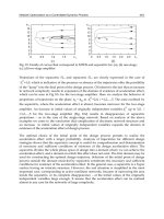
Fig. 10. Family of curves that correspond to MTDS and separatrix for: (a), (b) one-stage;
(c), (d) two-stage amplifier

Projections of the separatrix SL
1
and separatrix SL
2
are clearly expressed in the case of
0
i
x =1,0, which is indicative of the presence or absence of the trajectories offer the possibility
of the “jump” into the final point of the design process. Of interest is the fact that an increase
in network complexity results in expansion of the domain of existence of acceleration effect,
which can be seen in Fig 10c for the two-stage amplifier. Here we analyze the behavior of
projections of trajectories on the plane
105
xx
−
at
0
i
x =2,0, i =1,2,…,5. The zone confined by
the separatrix, where the acceleration effect is absent, becomes narrower for the two-stage
amplifier. An increase in initial values of originally independent variables
0
i
x
up to 3,0, i

=1,2,…,5 for the two-stage amplifier (Fig. 10d) results in disappearance of separatrix
projections – as in the case of the single-stage network. Based on analysis of the above
examples we come to the conclusion that complication of electronic network structure and
an increase in initial values of originally independent variables expands the domain of
existence of the acceleration effect of design process.

The optimal choice of the initial point of the design process permits to realize the
acceleration effect with a larger probability. Analysis of trajectories for different design
strategies shows that the separatrix concept is useful for comprehension and determination
of necessary and sufficient conditions of existence of the design acceleration effect. The
separatrix divides the whole phase space of design into a domain where we can achieve the
acceleration effect, and a domain in which this effect does not exist. The first domain may be
used for constructing the optimal design trajectory. Selection of the initial point of design
process outside the domain encircled by separatrix constitutes the necessary and sufficient
conditions for existence of the acceleration effect. In the general case, a separatrix is a hyper
surface having an intricate structure. However, the real situation is simplified in the most
important case, corresponding to active nonlinear networks, because of narrowing the area
inside the separatrix, or its complete disappearance – at the initial values of the originally
independent variables large enough. It means that the acceleration effect can be realized
almost in any case for the networks of large complexity.

444 Frontiers in Robotics, Automation and Control
6. Stability analysis

Basic concepts of a new methodology in analogue networks optimization in terms of the
control theory were stated in previous sections. It was shown that the new approach
potentially allows to significantly decreasing the processor time used to design the circuit.
This quality appears due to a new possibility of controlling the design process by
redistributing computational burden between the circuit’s analysis and the procedure of
parametric optimization. It may be considered to be a proven fact that traditional design

strategy (TDS) including the circuit’s analysis at every step of its design is not optimal with
respect to time. More over the benefit in time used to design the circuit for some optimal or
more precisely quasi-optimal strategy compared to TDS increases with increasing size and
complexity of the designed circuit. This optimal strategy and corresponding design’s
trajectory were obtained using special search procedure and serve only as a proof existing
strategies which are much more optimal than TDS. However, it is clear that the problem lies
in the ability to move along an optimal trajectory of the circuit’s design process from the
very beginning of designing the circuit. Only in this case it is possible to obtain the
mentioned potentially tremendous advantage in time, which corresponds to the optimal
design strategy. During the building the optimal strategy and its corresponding trajectory at
the present moment it is necessary to analyze their most significant characteristics. The
study of the optimal trajectory’s qualitative characteristics and their differences from those
of the other trajectories appears to be the only possible way to solve the problem.
The discovery of an effect expecting additional acceleration of the design process and
exploration of conditions determining this effect’s existence lead to increased time
advantage and serve as an initial point of quasi-optimal design strategy building. The
analysis of this effect allowed to state three most significant moments: 1) to obtain the
acceleration effect the initial point of the design process should be chosen outside the
domain limited with a special hypersurface (separatrix), 2) the acceleration effect appears
during a transition from a trajectory corresponding to a modified traditional design strategy
(MTDS) to the trajectory which corresponds to TDS and from any trajectory similar to MTDS
to any trajectory similar to the trajectory of TDS, 3) the most significant element of the
acceleration effect is an exact position of the switch point corresponding to a transition from
one strategy to another.
To obtain an optimal sequence of switching points during the design process it is necessary
to select a special criterion, which depends on the internal properties of the design strategy.
The problem of searching for the optimal with respect to time design strategy deals with a
more general problem of convergence and stability of each trajectory. On the basis of
experiment, the design time for each strategy determines by properties of convergence and
stability of corresponding trajectory. One of the common approaches of analysis of dynamic

systems stability is based on the direct Lyapunov method (Barbashin, 1967; Rouche et al.,
1977). We consider that the time design algorithm is a dynamic controlled process. In this
case, the main control aim is determined as minimization problem of transient time of this
process. As result, the analysis of stability and characteristics of transient process (process of
designing is one of these) for each trajectory are possible on the basis of the direct Lyapunov
method. Let’s introduce Lyapunov function of process of designing. It will be used for
analysis of properties and structure of optimal algorithm and for searching of optimal
switch point positions of control vector particularly.
Network Optimization as a Controllable Dynamic Process 445
There is a certain freedom of Lyapunov function choice as the latter has more than one form.
Let’s denote the Lyapunov function of process of designing (1)–(5) in form:


(
)
(
)
∑
−=
i
ii
axXV
2
(22)
where
i
a is a stationary value of coordinate
i
x . The set of all coefficients
i

a is the main
result of process of designing as the minimum of target function
(
)
XC is achieved at these
values of coefficients, i.e. the aim of designing is succeeded. It is clear, that these coefficients
are accurately known only at the end of designing. The other variables
iii
axy −
=
could
be determined instead of
i
x variables. In this case equation (5) takes the form:


(
)
∑
=
i
i
yYV
2
(23)
Taking into account the new variables
i
y , the process of designing (1)–(5) remains the same
form. However, equation (23) satisfies all conditions of Lyapunov function definition.
Indeed, this function is piecewise continuous function having piecewise continuous first

partial derivatives. In addition, three main properties of function (23) V(Y)>0, 2) V(0)=0, and
3)
()
∞→YV
for
∞→Y
) are presented. In this case we obtain the possibility to
analyze the stability of equilibrium position (point Y=0) by Lyapunov theorem. On other
hand, the stability of point
(
)
N
aaaa , ,,
21
=
analyzes on basis of (22). It is clear, both of
these problems are identical. The point
(
)
N
aaaa , ,,
21
=
can be defined only at the end
of the process of designing that is inconvenience of equation (22). As result, we could
analyze the stability of various designing strategies by the equation (22) if the problem’s
solution (i.e. point a) was determined already in another way. Moreover, the possibility to
control the stability of process during optimization procedure is of interest. In this case we
have to determine another form of Lyapunov function which would be irrespective of final
stationary point a. Let’s define Lyapunov function in the form:

(
)
(
)
[
]
r
UXFUXV ,, =
(24)


()
()
∑
⎟
⎟
⎠
⎞
⎜
⎜
⎝
⎛
∂
∂
=
i
i
x

UXF
UXV
2
,
,
(25)

where F( X,U ) is a generalize target function of process of designing and r > 0. Under
446 Frontiers in Robotics, Automation and Control
additional conditions both of these equations determine Lyapunov function having
properties similar to (23) in the sufficiently great neighborhood of stationary point.
Meanwhile the dependence on control vector U appears too. Indeed, we can see that the
value of (24) is equal zero in the stationary point if the target function of this process
()
XC

in the same point is equal zero as well. The equation (24) is positive defined function in all
points distinct from a stationary point as the function
(
)
XC
is nonnegative. The function
()
UXV ,
increases without bound when we are going away from the stationary point.
The equation (25) also determines Lyapunov function if
i
xF
∂
∂

/
= 0 in the stationary point
()
N
aaaa , ,,
21
= and V(a,U)=0. On the other hand, V(X,U)>0 for all X. In conclusion,
Lyapunov function determined by (25) is a function of vector U i.e. all coordinates
i
x
depend on U. The third property of Lyapunov function is proven wrong as the behavior of
function V(X,U) when
∞→X
is unknown. However, as known a posteriori, the
function V(X,U) is the increasing function in the sufficiently great neighborhood of a
stationary point. According to Lyapunov method, the information about trajectory stability
is connected with time derivative of Lyapunov function. Direct calculation of time
derivative of Lyapunov function
•
V
lets estimate the dynamic system stability. The process
of designing and a corresponding trajectory is stable if this derivative is negative. On the
other part, the direct Lyapunov method gives sufficient but not necessary stability
conditions. This implies that the process can lose stability or can remain stable in the case of
positive derivative. The appearance of positive values of derivative
•
V
on set of positive
measure only states the instability displaying in a few growth of Lyapunov function instead
of decreasing latter. If such process exists far from the stationary point, then the process of

designing is divergent function and we cannot obtain the solution of this trajectory. In this
case the initial point of process of designing or strategy should be changed. If the positive
derivative
•
V
appears at the end of process of designing (i.e. not far from the stationary
point), then we could say that the process of designing significantly decelerates. This
designing strategy is going round in a circle and cannot provide required accuracy. As
result, the engineering time substantially grows. This effect is well known in practical
designing. If we obtain the unacceptable accuracy, the strategy of designing or initial point
have to be changed. The detailed behavioral analysis of Lyapunov function and its
derivative for different strategies of designing makes it possible to choose the perspective
strategies. This analysis also allows determining on qualitative level the relationship
between design time and Lyapunov function and its derivative being the main factors of the
process of designing.
Two-stage transistor amplifier, depicted in Fig.3, is used for stability analysis of different
strategies of design. The direct calculation of time derivative
•
V
of Lyapunov function,
determined by (29) for r=0.5, shown that the derivative is negative in the initial point of
design for all trajectories, i.e., all possible design’s strategies and its trajectories are stable at
the beginning if integration step of system (1) is enough small. In the same time, when the
current point of trajectory reaches some
ε
-neighbourhood of the stationary point
Network Optimization as a Controllable Dynamic Process 447
()
N
aaa , ,,

21
, the derivative of Lyapunov function comes positive and the current
design’s strategy loses stability. This implies that this strategy dose not ensure the
convergence of trajectories to the stationary point
(
)
N
aaa , ,,
21
starting from some
value of
ε
-neighbourhood, i.e. achievement of minimum of target function F(X,U) and so
function C(X) with accuracy to
ε
dose not guarantee. In fact, each trajectory has eigen
ε
-
neighbourhood determining maximum available accuracy for this one and the convergence
problem arises inside this area. The process of designing significantly decelerates for current
strategy before approaching of the critical value of
ε
-neighbourhood. Alias, the derivative
•
V
remains negative but has enough small absolute value. The results for two-stage
amplifier are presented in Table 7. The design realized on the basis of strategies coming into
structural basis 2
M
and determined by control vector U. The appearance of positive values of

derivative
•
V
on set of positive measure determines the termination of process of designing.
Process optimization realized on the basis of equation (18) and gradient method with a
variable optimal step
s
t
hereupon this step
s
t could be both small and large. As result, we
have non-smooth behavior of derivative from one step to other.

Table 7. Critical value of the
ε
-neighborhood for design strategies for two-stage amplifier

For smoothing of derivative
•
V
the value averaging on the interval 30 steps was used. The
N Control vector Iterations Computer Critical value of
U(u1,u2,u3,u4,u5) number time (sec) -neighborhood
1 ( 0 0 0 0 0 ) 3177 7.25 2.78E-08
2 ( 0 0 0 0 1 ) 3074 8.02 3.36E-07
3 ( 0 0 0 1 1 ) 11438 26.36 8.18E-07
4 ( 0 0 1 0 1 ) 799 1.16 9.38E-09
5 ( 0 0 1 1 0 ) 1798 2.61 1.61E-08
6 ( 0 1 0 1 1 ) 43431 76.89 3.16E-05
7 ( 0 1 1 0 0 ) 1378 2.25 1.67E-08

8 ( 0 1 1 0 1 ) 571 0.72 6.83E-09
9 ( 0 1 1 1 0 ) 1542 2.03 2.05E-08
10 ( 1 0 0 1 1 ) 11839 21.37 1.68E-05
11 ( 1 0 1 0 0 ) 2097 3.57 5.47E-07
12 ( 1 0 1 1 0 ) 6026 8.31 4.94E-07
13 ( 1 1 1 0 0 ) 6602 8.84 7.41E-07
14 ( 1 1 1 0 1 ) 935 0.71 1.33E-08
15 ( 1 1 1 1 0 ) 2340 2.31 1.62E-07
16 ( 1 1 1 1 1 ) 1502 0.38 1.09E-08
ε
448 Frontiers in Robotics, Automation and Control
analysis of results of Table 7 has shown some important laws. First of all, the strong
correlation between processor time and critical value of
ε
-neighbourhood, after which the
value of derivative
•
V
stays positive, is presented. As a rule, the fewer available value of
ε

-neighbourhood corresponds to the fewer processor time. We could order all strategies in
Table 7. from the smallest processor time (0.38 sec, No. 16) to the longest one (76.89 sec, No.
6).
On the other hand, the strategies in ascending order of critical value of
ε
-neighbourhood
are presented in Table 8.

Table 8. Strategies’ ordering by processor time and by critical value of
ε
-neighborhood

The No. of each strategy in Table 8 determined by two different ways of order is slightly
different. Two strategies (13 and 6) have the same number. Seven strategies have the
difference in one place, four ones – in two places, and three strategies – in three places. The
average difference is equal to 1.5. Taking into account that the critical values of
ε
-
neighbourhood are obtained approximately by the averaging during integration of system
(1) we can see that the correspondence of processor time with critical value of
ε
-
neighbourhood is enough acceptable. Contrariwise, the parameters of
ε
-neighbourhood
are obtained on the basis of Lyapunov function and its derivative analysis. Therefore, we
could say that the strong correlation between processor time and properties of Lyapunov
function is presented.
From the analysis above the assumption is induced: Lyapunov function of process of
designing and its derivative are enough informative source to select more perspective
design strategies.

7. Conclusion

The traditional approach for the analogue network optimization is not time-optimal. The
problem of the minimal-time design algorithm construction can be solved adequately on the
basis of the control theory. The network optimization process in this case is formulated as a
controllable dynamic system. Analysis of the different examples gives the possibility to

conclude that the potential computer time gain of the time-optimal design strategy increases
when the size and complexity of the system increase. The Lyapunov function of the
optimization process and its time derivative include the sufficient information to select more
perspective strategies. The above-described approach gives the possibility to search the
Number 1 2 3 4 5 6 7 8 910111213141516
Number of strategie
s

regulated by the
computer tim 16 14 8 4 9 7 15 5 11 1 2 12 13 10 3 6
Number of strategie
s

regulated by the

-neighborhood 8 4 16 14 5 15 7 9 1 2 12 11 13 3 10 6
ε
Network Optimization as a Controllable Dynamic Process 449
time-optimal algorithm as the approximate solution of the typical problem of the optimal
control theory.

8. References

Barbashin, E.A. (1967). Introduction in Stability Theory, Nauka, Moscow
Brayton, R.K.; Hachtel, G.D. & Sangiovanni-Vincentelli, A.L. (1981). A survey of
optimization techniques for integrated-circuit design. IEEE Proceedings, Vol. 69, pp.
1334-1362
Fedorenko, R.P. (1969). Approximate Solution of Optimal Control Problems, Nauka, Moscow
Fletcher, R. (1980). Practical Methods of Optimization, John Wiley and Sons, New York, N.Y.
George, A. (1984). On block elimination for sparse linear systems. SIAM J. Numer. Anal., Vol.

11, No.3, pp. 585-603
Gill, P.E.; Murray, W. & Wright, M.H. (1981). Practical Optimization, Academic Press, London
Kashirskiy, I.S. (1976). General Optimization Methods. Izvest. VUZ USSR -Radioelectronica,
Vol. 19, No. 6, pp. 21-25
Kashirskiy, I.S. & Trokhimenko, Y.K. (1979). General Optimization for Electronic Circuits,
Tekhnika, Kiev
Massara, R.E. (1991). Optimization Methods in Electronic Circuit Design, Longman Scientific &
Technical, Harlow
Massobrio, G. & Antognetti, P. (1993). Semiconductor Device Modeling with SPICE, Mc. Graw
Hill, Inc., New York, N.Y.
Ochotta, E.S.; Rutenbar, R.A. & Carley, L.R. (1996). Synthesis of high-performance analog
circuits in ASTRX/OBLX”, IEEE Trans. on CAD, Vol. 15, No. 3, pp. 273-294
Osterby, O. & Zlatev, Z. (1983). Direct Methods for Sparse Matrices, Springer-Verlag, New
York, N.Y.
Pontryagin, L.S.; Boltyanskii, V.G.; Gamkrelidze, R.V. & Mishchenko, E.F. (1962). The
Mathematical Theory of Optimal Processes. Interscience Publishers, Inc., New York
Pytlak, R. (1999). Numerical Methods for Optimal Control Problems with State Constraints,
Springer-Verlag, Berlin
Rabat, N; Ruehli, A.E.; Mahoney, G.W. & Coleman, J.J. (1985). A survey of macromodeling.
Proc. IEEE Int. Symp. Circuits Systems, pp. 139-143, April 1985.
Rizzoli, V. Costanzo, A. & Cecchetti, C. (1990). Numerical optimization of broadband
nonlinear microwave circuits. IEEE MTT-S Int. Symp., Vol. 1, pp. 335-338
Rouche, N.; Habets, P. & Laloy, M. (1977). Stability Theory by Liapunov’s Direct Method,
Springer-Verlag, New York, N.Y.
Ruehli(a), A.E.; Sangiovanni-Vincentelli, A. & Rabbat, G. (1982). Time analysis of large-scale
circuits containing one-way macromodels. IEEE Trans. Circuits Syst., Vol. CAS-29,
No. 3, pp. 185-191
Ruehli(b), A.E. (1987). Circuit Analysis, Simulation and Design, Vol. 3, Elsevier Science
Publishers, Amsterdam
Sangiovanni-Vincentelli, A.; Chen, L.K. & Chua, L.O. (1977). An efficient cluster algorithm

for tearing large-scale networks. IEEE Trans. Circuits Syst., Vol. CAS-24, No. 12, pp.
709-717
Wu, F.F. (1976). Solution of large-scale networks by tearing. IEEE Trans. Circuits Syst., Vol.
CAS-23, No. 12, pp. 706-713
450 Frontiers in Robotics, Automation and Control
Zemliak(a), A.M. (2001). Analog system design problem formulation by optimum control
theory. IEICE Trans. on Fundam., Vol. E84-A, No. 8, pp. 2029-2041
Zemliak(b), A.M. (2002). Acceleration Effect of System Design Process. IEICE Trans. on
Fundam., Vol. E85-A, No. 7, pp. 1751-1759