Robotics Automation and Control 2011 Part 10 docx

Control of Redundant Submarine Robot Arms under Holonomic Constraints

261
3.1 The AUV model
The model of a submarine can be obtained with the momentum conservation theory and
Newton’s second law for rigid objects in free space via the Kirchhoff formulation (Fossen),
the inclusion of hydrodynamic effects such as added mass, friction and buoyancy and the
account of external forces/torques like contact effects (Olguín Díaz). The model is then
expressed by the next set of equations:
),,()(),()(
)(
tvFuqgvtvDvvCvM
vv
v
cvvvvvvvvvv
η
++=+++


(1)

(2)
From this set, (1) is called the dynamic equation while (2) is called the kinematic equation.
The generalized coordinates vector q
v
∈ ℜ
6

is given on one hand by the 3D Cartesian position
d
v

= (x
v
, y
v
, z
v
)
T
of the origin of the submarine frame (Σ
v
) with respect to a inertial frame (Σ
0
),
and on the other hand by any set of attitude parameters that represent the rotation of the
vehicle’s frame with respect to the inertial one. Most common sets of attitude representation
such a Euler angles, in particular roll-pitch-yaw (φ, θ, ψ), use only 3 variables (which is the
minimal number of orientation variables). Then, for a submarine, the generalized
coordinates represents its 6 degrees of freedom:

(3)
where ϑ
v
= (φ
v
, θ
v
, ψ
v
)
T

stands for the attitude parameter vector.
The vehicle velocity ν
v
∈ ℜ
6
is the velocity wrench (vector representing both linear and
angular velocity) of the submarine in the vehicle’s frame. This vector is then defined as

The relationship between this vector and the generalized coordinates
is given by the kinematic equation. The linear operator J
v
(q) ∈ℜ
6
×
6
in (2), is built by the
concatenation of two transformations. The first is J
q
(q
v
) ∈ℜ
6
×
6
which converts time
derivatives of generalized coordinates to velocity wrench in the inertial frame. This operator
is necessary because the angular velocity of a body (ω) is not given by the time derivative of
its angular parameters (

≠ ω). However, there is always a transformation operator given by
the very specific type of chosen orientation parameters:

(4)
Then the operator J
q
(q
v
) is defined as:

(5)
The second operator is
Robotics, Automation and Control

262

(6)
which transforms a 6 dimension tensor from the inertial frame to vehicle’s frame. The matrix
R
v
0
(ϑ
v
)

∈ SO
3
is the rotation matrix of the vehicle. Thus, the linear operator is defined as

A detailed discussion on the terms of (1) can be found in (Olguín Díaz & Parra-Vega).

In the dynamic equation (1), matrices M
v
,C
v
(ν),D
v
(·) ∈ℜ
6
×
6
are Inertia matrix, Coriolis matrix
and Damping matrix. M
v
includes the terms of classical inertia plus the hydrodynamic
coefficients of the added mass effect (due to the amount of extra energy needed to displace
the surrounding water when the submarine is moving). The Inertia matrix is constant,
definite positive and symmetric only when the submarine is complete immersed and the
relative water incidence velocity is small (Fossen). This condition is met for a great amounts
of activities. The Coriolis vector C
v
(ν)ν represents the Coriolis and gyroscopic terms, plus the
velocity quadratic terms induced by the added mass. The Coriolis matrix in this
representation does not depend on the position but only on the velocity, in contrast to the
same expression for a Robot Manipulator. It is indeed skew symmetric and fulfills the classic
relationship for Lagrangian systems:
M

v
−2C
v

(ν) = Q; Q+Q
T

= 0. The Damping matrix
represents all the hydrodynamic effects of energy dissipation. For that reason it is a strictly
positive definite matrix, D
v
(q, ν, t) > 0. Its arguments are commonly the vehicle’s orientation
ϑ
v
, the generalized velocity ν, and the velocity of the surrounding water ζ(t). The diagonal
components represents the drag forces while the off-diagonal components represent the lift
forces. Vectors g
v
(q), u,
()
c
F
v
∈ℜ
6
are all force wrenches (force-torque vector) in the vehicle’s
frame. They represent respectively: gravity, input control and the contact force. Gravity
vector includes buoyancy effects and it does not depend on velocity but on the orientation
(attitude) of the submarine with respect to the inertial frame. The contact force wrench is the
one applied by the environment to the submarine. The input control are the forces/torques
induced by the submarine thrusters in the vehicle frame.
The disturbance η
v
(ν, ζ(t),


ζ
(t))of the surrounding fluid depends mainly in the incidence
velocity, i.e. the relative velocity of the vehicle velocity and the fluid velocity. The last is a
non-autonomous function, but an external perturbation. This disturbance has the property
of

(7)
That is that all the disturbances are null when the fluid velocity and acceleration are null.
The dynamic model (1)-(2) can be rearranged by replacing (2) and its time derivative into
(1). The result is one single equation model:

(8)
Control of Redundant Submarine Robot Arms under Holonomic Constraints

263
which, whenever

has the form of any Lagrangian
system. Its components fulfills all properties of such systems i.e. definite positiveness of
inertia and damping matrices, skew symmetry of Coriolis matrix and appropriate bound of
all components (Sagatun & Fossen). The control input in this equation is obtained by a linear
transformation of the real input using the linear operator given by the kinematic equation:

(9)
The contact effect is also obtained by the same transformation. However it can be expressed
directly from the contact wrench in the inertial frame (Σ
0
) by the relationship

(10)
where the contact force
(0)
c
F
is the one expressed in the inertial frame. By simplicity it will be
noted as F
c
from this point further. The relationship with the one expressed in the vehicle’s
frame is given by
This wrench represents the contact forces/torques
exerted by the environment to the submarine as if measured in a non moving frame. These
forces/torques are given by the normal force of an holonomic constraint when in contact
and the friction due to the same contact. For simplicity in this work, tangential friction is not
considered. The equivalent of the disturbance is obtained also with the linear operator given
as:

(11)
3.2 Contact force due to an holonomic constraint
A holonomic constraint (or infinitely rigid contact object) can be expressed as a function of
the generalized coordinates of the submarine as

(12)
with φ(q
v
) ∈ℜ
r
, where r stands for the number of independent contact points between the
SRA and the motionless rigid object. Equation (12) means that stable contact appears while
the SRA submarine does not deattach from the object φ(q

v
) = 0. Evidently all time
derivatives of (12) are zero, which for r = 1

(13)
where
is the constraint jacobian. Last equation means that velocities of
the submarine in the directions of constraint jacobian are restricted to be zero. This
directions are then normal to the constraint surface φ(q
v
) at the contact point. As a
consequence, the normal component of the contact force has exactly the same direction as
those defined by J
φ
(q
v
), consequently, the contact force wrench can be expressed as

(14)
Robotics, Automation and Control

264
where

is a normalized version of the constraint jacobian; λ∈ℜ
r
is the magnitude
of the normal contact force at the origin of vehicle frame: λ =
c
F

. The free moving model
expressed by (1)-(2), when no fluid disturbance and in contact with the holonomic constraint
can be rewritten as:

(15)


(16)


(17)
where
Equivalently, the model (8) is also
expressed as

(18)

(19)
with
Equations (18)- (19) are a set of Differential Algebraic Equations index 2 (DAE-2). To solve
them numerically, a DAE solver is required. This last representation has the same structure
and properties as those reported in (Parra-Vega).
3.3 The robot arm
This section formulates the problem of a manipulator having free mobility on its base. That
means, when the base of the robot arm is no longer inertial and thus does not fulfils
Newton’s laws unless all its dynamic is at new, expressed in a inertial frame.
In order to include the movent of the base of the robot arm, it is necessary to introduce some
extra elements which do not appear in the classical fixed-base model. For this case, the free
moving base, the inertial frame shall be chosen in the same way it is chosen for the vehicle’s:
at some point attached to the earth. It is evident that this two references can be identical for

the fixed base case, but should certainly be different for the free moving base case. Lets use
the inertial reference Σ
0
used for the submarine and define as Σ
b
the base frame of the arm
when its base is no moving, known as the fixed-base condition.
As a result there are two new homogeneous transformations in the kinematic chain: H
v
0
(q
v
)
from

inertial frame Σ
0
to the vehicle’s frame Σ
v
and H
b
v

from Σ
v
to the fixed-base first
reference frame Σ
b
from which all the modelling is obtained.
The homogeneous transformation from inertial frame Σ

0
to the vehicle frame Σ
v
is then given by:


(20)
where d
v
is the inertial position of the vehicle and R
v
0

∈SO
3
represents its orientation. Recall
that the generalized coordinates of the vehicle are given in (3).
Control of Redundant Submarine Robot Arms under Holonomic Constraints

265
The homogeneous transformation from Σ
v
to Σ
b
is then given by:


(21)
where d
b/v

∈ℜ
3

is the position vector of b wrt vehicle’s frame (expressed in Σ
v
) and R
b
v
∈ SO
3
represents the orientation that the arm is attached to the vehicle. With the reasonable
assumption that the vehicle is a rigid body, and that the assembling is as well, this
transformation is constant.
The forward kinematics of the free-base robot arm is given by the concatenation of the
proper homogeneous transformations. For instance, the forward kinematic of the end-
effector x
e
is given by:

where H
e
b

(q
m
) stands for the homogeneous transformation of the manipulator , and q
m
are
the generalized coordinates of the arm chain, both under the fixed-base conditions.
From here on, it is evident that the generalized coordinates for the free-base manipulator

shall be extended to include the vehicle configuration as

(22)
An acceptable interpretation is that the vehicle is an extra link in the manipulator’s chain
that has a six degree-of-freedom articulation.
The forward kinematics of the end-effector are given by:

(23)


(24)
where
is the forward kinematic equation on the the fixed-base condition, and

is the position vector of the end-effector from the origin of the vehicle’s frame,
expressed in that same frame Σ
v
.
From eqs. (23)-(24) the linear inertial velocity of the end-effector is:

(25)
The linear velocity
is the fixed-based condition’s linear velocity of the end-effector
and can be calculated via the linear velocity jacobian:

Then last
relationship can also be expressed as

(26)
Robotics, Automation and Control

266
The angular velocity of the end-effector is the sum of the vehicle’s angular velocity ω
v
plus
the relative angular velocity of the end-effector respect to the base ω
e/b
expressed in the
inertial frame. Then, the angular velocity of the end-effector is:

(27)
where
is the angular velocity jacobian for the fixed-base condition. By replacing
equation (4) in equations (26) and (27), the end-effector velocity wrench can be written as a
function of the extended generalized coordinates and its time derivative as:

(28)
Last equation can also be written in block matrices in the next way:






(29)


(30)
(31)
where the vehicle Jacobian J

v
∈ℜ
6
×
6
is defined as:

(32)
and the manipulator Jacobian J
m
∈ℜ
6
×
n
is defined as:

(33)
In the above definitions, the term [a×] stands for the skew symmetric matrix representation
of the cross product of a vector (Spong & Vidyasagar), J
b
R
∈SO
6
is defined as (6) and J
fb
is the
manipulator fixed-base geometric Jacobian. The geometric version of the vehicle Jacobian
J
v
g

(ϑ
v
, q
m
) and the manipulator Jacobian J
m
(ϑ
v
, q
m
) make up the Mobile Manipulator
Jacobian defined in (Hootsman & Dubowsky). However, in this work we prefer to use this
geometric jacobian because it maps the generalized velocities q

in linear an angular
velocities at any point in the vehicle/ manipulator system.

(34)
The dynamics of the free base manipulator can be obtained using the expressions of the
kinetic and potential energy of any mass, and using expressions (23) and (29). Because the
Control of Redundant Submarine Robot Arms under Holonomic Constraints

267
generalized coordinates vector has a 6 + n dimension, there must be an inertia matrix
H
(q)
of the size (6 + n) × (6 + n) and the vector of generalized forces  should also have a 6 + n
dimension.
The kinetic energy of a free-base manipulator is given by:

(35)

(36)
where the body 0 is the base, that has no movement in the fixed-base conditions. The linear
velocity
d

ci
and ω
i
are given by equations (26) and (27), respectively, but calculating the
distance to the center of mass of the corresponding link.
The resulting solution for this extended inertia matrix can be written as follows:

(37)
which by definition is symmetric and definite positive.

(38)

(39)

(40)
Note that Matrix H
fb
is the inertial matrix of the same robot arm for the fixed-base condition
and it depends only in the manipulator coordinates q
m
.
On the other hand, being the potential energy, gravitational and buoyant is also function of

the vehicle positions, it can be written as a function of the generalized coordinates:

(41)
Then the dynamic equation can be obtained by solving the Euler-Lagrange equation. The
resulting model would be of the form:

(42)
where

is the Coriolis matrix which has the same properties that for
the fixed-base case (i.e.
always true),

is the
Robotics, Automation and Control

268
gravitational vector of the manipulator and its influence over the vehicle’s coordinates and
includes the restoring forces due to the floatability of each link,
τ
q
is the generalized
coordinates force vector, and
τ
hydro
are the generalized forces due to the hydrodynamic
effects.
This last term is somehow complicated to determine. However, a good approximation is to
compute these forces over each link and to translated them to the generalized coordinates,
using the virtual work principle (Spong & Vidyasagar), by means of the Mobile Manipulator

Jacobian (34) of the geometric center of each link. The resulting vector shall have the next
structure (Olguín Díaz):

where the damping matrix D
m
>0 is positive definite, due to the fact that the hydrodynamic
effects are dissipative, and the hydrodynamical perturbation forces
η
m
becomes null when
the current is steady (ζ(t) =

ζ = 0). The Damping matrix D
m
(·) can be also be written in
block submatrices as:

Coriolis, gravitational terms, Hydrodynamic damping and current perturbations are highly
nonlinear so it is very common to write then together as the non-linear vector
Then model (42) can be presented
as a function of vehicle’s and arm’s coordinates q
v
and q
m
:

(43)
Or else, it can be written as two coupled equations as:

(44)

(45)
3.4 The submarine AUV+Robot Arm=SRA
The interaction between the models of the vehicle and the free-base manipulator are forces-
torques at the attaching point. So if the original assumption where this attachment is rigid,
i.e. it does not nave elastic deformation behaviour, this force wrench shall appeared in both
models with opposite direction (due to Newton’s 3rd law).
On one hand, this interaction wrench is given in the vehicle dynamics as an external
perturbation wrench. This can be seen in the dynamic equation (8) as follows:

(46)
where
is the non-linear
vector term and 
arm
is the perturbation produced by the manipulators movements interaction.
Control of Redundant Submarine Robot Arms under Holonomic Constraints

269
On the other hand, the interaction between the vehicle and the arm, seen from the
manipulator is the component 
m/v
on either model (43) or (44). By Newton’s 3
rd
law it can be
seen that the force wrench 
m/v
on the manipulator model is the same but with opposite
direction of the perturbation 
arm

on the vehicle’s model.

(47)
Then by using last equality, a single expression for both model (44) and (46) is found to be:

(48)
Then equations (45) and (48) can be represented by a single whole-system differential
equation in a compact form by a coupled pair of differential equations:

(49)
where the nonlinear terms can also be written in a compact form as
and the overall terms are given by the
next set of relationships [6]:

(50)

(51)


(52)


(53)


(54)

(55)
As well as inthe case of the AUV alone, whenever ζ(t) =
ζ


(t) = 0, then )(·) = 0,and the
dynamic equation (49) has the form of a Lagrangian system. Thus, its components fulfills all
properties of such systems i.e. definite positiveness of inertia and damping matrices, skew
symmetry of Coriolis matrix and appropriate bound of all components.
3.5 SRA in contact
When the end-effector of the SRA gets in contact with the environment, external forces and
torques appear in the dynamics that was not taken into account when the dynamics
Robotics, Automation and Control

270
equations was obtained. Let
express the force wrench due to
contact forces and torques at the end-effector.

From the virtual work principle, this contact
force F
e
will modify the dynamics of the system through the transpose of the Mobile-
Manipulator-Jacobian given by equation (34) as

(56)
Which means that the contact forces are translated to the vehicle coordinates by the vehicle’s
Jacobian and to the joints by the manipulator’s Jacobian.
Then equation (49) is modified by adding 
c
as an external force to the righthand side
yielding to

(57)

In this work, this contact force is also modelled in the same manner as treated in section 3.2, as

(58)
Where the J
φ
(q)=J
φ+
(q)J(q) is the jacobian of the holonomic restriction and λ is the magnitude
of the contact force.
4. Open-loop error equation
The introduction of a so called Orthogonalization Principle has been a key in solving, in a
wide sense, the force control problem of a robot manipulators with fix base. This physical-
based principle states that the orthogonal projection of contact torques and joint generalized
velocities are complementary, and thus its dot product is zero, carrying no power and no
work is done. Relying on this fundamental observation, passivity arises from torque input to
generalized velocities, in open-loop. To preserve passivity in closed-loop, then, the closed-
loop system must satisfy the passivity inequality for a given error velocity function. This is
true for robot manipulators with fixed frame, and here we extend this approach for robots
whose reference frame is not inertial, like SRA. Additionally, we present here the
developments that this holds true also for redundant SRA.
4.1 Orthogonalization principle and linear parametrization
Similar to (Liu et al.), the orthogonal projection of J
φ
(q), which arises onto the tangent space
at the contact point, is given by the following operator
(6+n)x(6+n)

(59)
where I
6+n

∈ℜ
(6+n)x(6+n)
is the identity matrix and , which always exists
since

rank{J
φ
(q)} = r. Notice that
{
}
() (6 )rank Q q n r
=
+−
and Qq q
=

, then Q(q)
t
J
ϕ
(q)=0.
Therefore,

according to the Orthogonalization Principle, the integral of (, q

) is upper
bounded by −H(t
0
), for

H(t) = K + P whenever because
Control of Redundant Submarine Robot Arms under Holonomic Constraints

271
Then passivity arise for the

full constrained SRA, under no fluid disturbances. This
conclusion gives a very useful and promising

theoretical framework, similar to the approach
of passivity-based control for fix-base robot arms. On

the other hand, it is known that the
dynamic equation (49) with no fluid perturbation can be linearly parameterized as follows

(60)
where the regressor
is composed of known nonlinear functions and
Θ∈ℜ
p

by p unknown but constant parameters. This is useful to obtain the fundamental
change of coordinates of the SRA into the controlled error system, the system expressed in
error coordinates, wherein we want to control the system in the trivial equilibria.
4.2 Change of coordinates
In order to design the controller, we need to work out the open loop error equation using
(60), in terms of nominal references
q


r
, as follows. Consider

(61)
where
q

r
is the time derivative of q

r
, to be defined. Then the open loop (49) can be written by
adding and subtracting (61) as

(62)
where s ≡ q

− q

r
is called the extended error. The problem of designing a controller for the
open loop error equation (62) is to find u
q
such that s(
*
) exponentially converges when Y
r
Θ is
not available.
4.3 Kinematic redundancy

Notice that

(63)
Since dimensions of X∈ℜ
m
and q are not the same, jacobian J(q) ∈ℜ
m
×
(6+n)
, then its inverse
does not exists, then to obtain the inverse mapping of (63), we use the pseudoinverse of
Penrouse to get

(64)
where matrix
stands for the orthogonal projection of J(q) and
spans the 6 + n − m kernel of J(q), that is J(q) and Q
k
are orthogonal complements and its dot
product is zero. Now, let consider that Q
k
maps any arbitrary vector v ∈ℜ
(6+n)
into the null
space of J(q). Consider, let

(65)
Robotics, Automation and Control

272

be a vector which belongs to the null space of J(q). This vector yields

(66)
which means that (64) can be written as

(67)
That is, given m values of X, we can complete the remaining 6 + n - m values of q ∈ℜ
6+n
by
designing
z

under a given criteria.
4.4 Orthogonal nominal reference
Since
q

= Q q

, and considering the decomposition (67) to design the extended error
s =
q

−
q

r
≡ Q
q


−
q

r
, and aiming at preserving passivity in closed loop, it is natural to
consider a structure for
q

r
similar to q

, that is the nominal reference q

r
at the velocity level
takes de following form

(68)
with

(69)
where , X
d
(t) and λ
d
(t) are the desired smooth trajectories of position and
contact force
λ

ˆ

=
λ(t) − λ
d
(t) as the position and force tracking errors, respectively.
Parameters β, , γ
1
and γ
2
are constant matrices of appropriate dimensions; and sgn(y) stands
for the entrywise signum function of vector y, and

(70)

(71)

(72)

(73)

(74)

(75)

(76)

(77)
Control of Redundant Submarine Robot Arms under Holonomic Constraints

273
for  > 0, η > 0. Finally, the reference for

z

, that is z

r
introduces a reconfigurable error, such
that tracking errors in the null space will also converge to its desired value and full control
on the redundancy is introduced. To this end, consider

(78)
where
z

r
fulfills Q
k
z

r
= z

r
in such a way that

(79)

(80)

(81)

(82)
for positive definite feedback gains
To complete the definitions, consider

(83)
where
stands for the gradient of a given cost function Ω to be optimized.
According to

this cost function, the redundant degrees of freedom of the full open kinematic
chain tracks
z

d
and z
d
, as it will be proved in the following, where


(84)
for without loss of generality it is assumed that z
d
(t
0
) = q(t
0
). Finally, owing to the fact that
and that s
r
=

q

−
q

r
, we obtain then

(85)

(86)
where s
vp
, s
vF
, and s
vz
respectively, are given by (73), (77) and (82). Notice that J
†
s
vp
and s
vz
are orthogonal complements (J
†
s
vp
)
T
s

vz
= 0 and so does Q(
*
) and
T
J
ϕ
. Notice that although
the time derivative of
q

r
is discontinuous, that is not of any concern because it is not used in
the controller.
5. Model-free second order sliding mode controller
Consider the following nominal continuous control law:


(87)
Robotics, Automation and Control

274
with
(6+n)x(6+n)
.
This nominal control, designed in the q-
space can be

mapped to the original coordinates of the vehicle model, expressed by the set
(1)-(2), using the next

relationship Thus, the physical controller in the
vehicle u
v
is implemented in terms

of a key inverse mapping J
-T
v
.

5.1 Closed-loop system
The open loop system (62) under the continuous model-free second order sliding mode
control (87) yields to

(88)
where
is useful for the passivity analysis.
5.2 Stability analysis
Theorem Consider a constrained SRA (57)under the continuous model-free second order
sliding mode control (87). The Underwater system yields a second order sliding mode
regime with local exponential convergence for the position, and force tracking errors.
Proof. A passivity analysis
indicates that the following candidate Lyapunov function
V qualifies as a Lyapunov function

(89)
for a scalar β > 0. The time derivative of the Lyapunov candidate equation immediately
leads to

(90)
where it has been used the skew symmetric property of
the boundedness of
both the feedback gains and submarine dynamic equation (there exists upper bounds for
the smoothness of φ(q) (so there exists upper bounds for J
φ
and
Q(q)), and finally the boundedness of Z. All these arguments establish the existence of the
functional ε. Then, if K
d
, β and η are large enough such that s converges into a neighborhood
defined by ε centered in the equilibrium s = 0, namely as t →∞, one obtains
s→ε (91)
This result stands for local stability of s provided that the state is near the desired trajectories
for any initial condition. This boundedness in the L
∞
sense, leads to the existence of the
constants ε
3
> 0, ε
4
> 0 and ε
5
> 0 such that

(92)
Control of Redundant Submarine Robot Arms under Holonomic Constraints

275

(93)
(94)
An sketch of the local convergence of s
vp
is as follows
1
. Boundedness of s

means
boundedness of the projected vectors then if we multiply them we get
zero, then we can analyze independently each projected vector. Locally, in the n − r
dimensional image of Q, we have that
Consider now that under an abuse
of notation that
such that for small initial conditions, if we multiply the
derivative of s
vp
in (73) by we obtain

(95)
which have used (92), and γ
1
> ε
3
, to guarantee the existence of a sliding mode at s
qp
(t) = 0 at
time
and according to the definition of s
qp

(72), s
qp
(t
0
) = 0, which
simply means that s
qp
(t) = 0 for all time.
Similar than for s
vp
, if we multiply the derivative of s
vz
in (79) by s
T
qz
, we obtain


(96)
which have used (93), and γ
z
> ε
4
, to guarantee the existence of a sliding mode at s
qz
(t) = 0 at
time and according to the definition of s
qz
in (79)-(82), s
qz

(t
0
) = 0,
which simply means that s
qz
(t) = 0 for all time.
Finally, we see that if we multiply the derivative of (77) by s
T
v
f
, we obtain

(97)
which have used (94), and γ
2
> ε
5
, to guarantee the existence of a sliding mode at s
qp
(t) = 0 at
time
and,according to (77), s
qF
(t
0
) = 0, which simply means that
s
qf
(t) = 0 for all time, which simply implies that λ→λ
d

exponentially fast.
6. Simulation results
Simulations has been made on a simplified and idealized platform of a 6 dof submarine with
a mass of 100 kg, where the floatability point it is assumed to be in the geometrical centre of
the vehicle. It is also assumed that the vehicle has neutral floatability i.e. the buoyancy forces
equals the gravity ones. The submarine vehicle was modeled as a regular cube, so its
principal moments of inertia are represented by a constant diagonal matrix. In order to get a
simple but reliant dynamic model, we considered the base of the robot arm to be in the
geometrical center of the vehicle. This robot arm was based on the 6 DoF Mitsubishi PA-10
with a mass of 30 kg. We also assumed that the spherical wrist only contributes in
orientation, that is, the last link has length zero. The robot arm principal moments of inertia
are as well assumed to be diagonal matrices.

1
The strict analysis follows (Liu, et. al.)
Robotics, Automation and Control

276
Now even when our simulator is simple, it contains most of the coupled dynamics from the
vehicle and the robot arm, which still makes the control problem quite a challenge.
Simulations were realized using the simulation software 20Sim 4.0, on a 64-bit Windows
Vista computer with 4 GB RAM memory at 2.1 GHz Dual-Core processor. Simulator
presents tridimensional results (x, y, z, roll, pitch, yaw), so the generalized coordinates for
the vehicle is given by:

(98)
which represents the cartesian position and orientation of the vehicle. The generalized
coordinate for the robot arm is given by:

(99)

which represents the manipulator joint positions. The generalized coordinates for the SRA
system is composed by the vehicle and robot arm generalized coordinates, and is given by:

(100)
The holonomic constraint is given by a vertical surface located at 1 meter from the origin,
who’s expression is

(101)
It is assumed that the SRA end-effector remains in contact with the environment for all the
time. In order to satisfy the constraint equation, the initial conditions were chosen as:

(102)

(103)
which leads to the following end-effector initial pose:

(104)
Now, the desired end effector position and orientation trajectory task are defined as:

(105)

(106)
On the other hand, the desired force profile applied by the SRA end effector on the contact
surface (holonomic constraint) is represented by:

(107)
Control of Redundant Submarine Robot Arms under Holonomic Constraints

277
The model-free control parameters are as follows:

And the force scalar gains were defined as η = 2, γ
2
= 10
−
1
.
6.1 Numerical considerations
To compute the value of λ, the constrained Lagrangian that fulfils the constrained
movement, can be calculated using the second derivative of the holonomic restriction:

φ
(q) = 0. Then, by using the dynamic equation (49) and after some algebra its expression
becomes either:

(108)
The set of eqns. (49)-(108) describes the constrained motion of the SRA when in contact to
infinitely rigid surface described by (12). Numerical solutions of these sets can be obtained
by simulation, however the numerical solution, using a DAE solver, can take too much
effort to converge due to the fact that these sets of equation represent a highly stiff system.
In order to minimize this numerical drawback, the holonomic constraint has been treated as
a numerically compliant surface which dynamic is represented by

(109)
This is known in the force control literature of robot manipulators as constrained
stabilization method, which bounds the nonlinear numerical error of integration of the
backward integration differentiation formula. With a appropriate choice of parameters P
and D, the solution of φ(, t) → 0 is bounded. This dynamic is chosen to be fast enough to
allow the numerical method to work properly. In this way, it is allowed very small

deviation on the computation of λ, typically in the order of −10
6
or less, which may produce,
according to some experimental comparison, less than 0.001% numerical error. Then, the
value of the normal contact force magnitude becomes:
Robotics, Automation and Control

278

(110)

Figure 1. Holonomic constraint using the constraint stabilizer
6.2 Model free position-force tracking control
Figure 2 shows the end-effector’s cartesian position. It is important to remark that the end-
effector x = 1 position, correspond to the holonomic constraint, which is asumued to be
satisfied for all the time, that because of the infinitely rigid object assumption given in in
(12). On the other hand, the y, z positions are the desired end effector trajectories over the
contact surface. Note that all the end effector positions are given in the inertial frame.


Figure 2. End-effector tracking desired position y, z while remaining in contact with the
holonomic constraint all the time.
On Figure 3 we find the end-effector orientation angles, which were defined as the roll-
pitch-yaw angles around the x-y-z axis of the inertial frame. It can be seen that orientation
tracks a desired orientation with all angles at at constant values of 0 for the roll and yaw
angles, and 3π/4 for the pitch angle.
Control of Redundant Submarine Robot Arms under Holonomic Constraints

279

Figure 3. End-effector’s orientation angles (roll, pitch, yaw), where we can see that set-point
tracking tasks on 0 and 3π/4 rad are being performed by the system.
Figure 4 shows how the end effector linear velocity vector evolves over time. In this Figure,
we can observe that x velocity remains on 0, while the y and z velocities tracks
1/10cos(t/10) and 0.05cos(t/2) respectively. This way, both set-point control and tracking
are being performed by the system.


Figure 4. End-effector linear x-y-z velocities, where both, regulation and tracking are
performed
Given the parameters used to describe the end-effector orientation, Figure 5 shows the time
derivative of these orientation parameters, which in the strictly mathematical sense, are
different form the end-effector angular velocity. In this figure, we can see that the
orientation derivative, after a small transient finally establish at zero radians, that is, the end
effector orientation will remain in the same position for all the time.
Now, let us define X as the 6 dof end-effector pose (position and orientation) vector, and
X

= X − X
d
as the pose error vector. Figure 6 shows the Euclidean norm of the end effector
Robotics, Automation and Control

280
pose error (&
X

&) and the norm of the end effector analytic velocity error (&
X



&), which
must not be confused with the geometric velocity error. In this figure, it is very clear that
the error manifold are nearly zero, because of the controller inner properties.

Figure 5. End-effector variation of angle parameters (
,,
θ

φψ) converge to zero after a small
transient

Figure 6. Euclidian norms of the end-effector’s pose and its time derivative (
X

,
X


), where
it is very clear the stability properties of the controller
Similarly as with the position, we defined a force task which must be accomplished by the
end effector when moving around the contact surface. This task is independent from the
position one, in other words, we can control both position and force simultaneous and
independently. Figure 7 presents the end-effector force tracking trajectory (λ), where a
periodic signal mounted on an offset of 100 N is shown. Additionally, Figure 7 shows on the
right upper frame, a zoom of how the contact force, tracks the desired force profile. On the
right lower frame, we can see the norm of the contact force error which is defined as
&
λ


& = &λ− λ
d
&. This error shows how fast the controller makes the contact force to track,
with very little error, the desired contact force trajectory.
In relation with the control signals, Figure 8 shows the x-y-z linear forces applied to the
vehicle. On this set of figures we can observe that no linear forces present chattering. This
Control of Redundant Submarine Robot Arms under Holonomic Constraints

281
characteristic is very representative of the second order sliding mode controllers. Note that
the biggest control signal belongs to the x linear force, this because of the shared
contribution of the vehicle and the manipulator to achieved the contact force on the
holonomic constraint, positioned along the x axis.


Figure 7. Left frame shows the end-effector contact force trajectory (λ), right upper frame
shows a zoom of this force, and the right lower frame shows the norm of the end effector
contact force ||
λ

||

Figure 8. The x-y-z linear inertial forces applied to the vehicle, where the contact force
contribution is mainly made through the x linear force
The vehicle torque control inputs can be seen in Figure 9, where, just as in the linear force
case, no chattering is present on the signals. In this figure, we can see that x and z torque
inputs are nearly cero, contrary to the y torque input, whose value oscillates around -30 Nm.
due to the torque created by the distance of the contact point to the vehicle’s origin.
Likewise, Figure 10 shows the torques (

i
) applied to the robot arm joints, where torque
inputs 
4
, 
5
, 
6
are nearly cero, this is because these three joints only contribute on the end
effector orientation in other words, the final link connected to them has length zero. Note
that joint torque 2 are the one that mostly contribute to the end effector contact force.
Now, Figures 11-14 show the generalized coordinates sliding surfaces, that is, the vehicle
and manipulator generalized coordinates surfaces. On these figures it can been shown that
the error manifolds converge to a stable bounded neighborhood centered in the origin. We
Robotics, Automation and Control

282
know that even when actual modern actuators have been growing really fast in past few
year, it is still imposible to implement a signum function on them, that is the main reason
why a saturation function is preferred. With the use of this saturation function we may no
get ideal results, instead we get this convergence region where error stabilize.



Figure 9. Input torques (n
x
, n
y
, n
z

) applied to the vehicle, where we can see that n
x
and n
z
are
nearly cero



Figure 10. Input control torques (
i
) applied to the robot-arm, where the contact force
contribution is mainly made through joint 2
On the other hand, Figure 15 shows the force error manifold, on which can be seen that the
force error converge to a stable bounded neighborhood centered in the origin. It is very clear
that this force manifold is the strongest one on the controller.
In consequence of the highly redundancy of the submarine robot arm (12 dof) working in
normal operational conditions (6 dof), some degrees of freedom can be used to perform an
additional task like minimize energy consumption, maximize dexterity, maximize the
Control of Redundant Submarine Robot Arms under Holonomic Constraints

283
distance to the mechanical limits, etc. These additional tasks can be made by projecting a
vector into the null space of the jacobian matrix.
Using the very know result of the gradient descendent, we can locally optimize a
performance criteria like the ones already mentioned.

Figure 11. Generalized coordinates 1-3 position sliding surface




Figure 12. Generalized coordinates 4-6 position sliding surface

Robotics, Automation and Control

284


Figure 13. Generalized coordinates 7-9 position sliding surface





Figure 14. Generalized coordinates 10-12 position sliding surface
Simulations results are presented using the distance to the mechanical limits as the
performance criteria, this criteria is given by:

(111)
where q
iM
(q
im
) represents the maximum (minimum) limit for the generalized coordinate q
i
,

and q
i
is the medium point for a coordinate range.
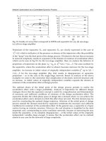
Figure 16 shows the performance criteria locally optimized for the required position-force
trajectory, where curve lower minima represents a local optimal configuration.
Control of Redundant Submarine Robot Arms under Holonomic Constraints

285


Figure 15. Force sliding surface
7. Remarks
There are several discussions that arise in such a complex system. In particular the dynamic
model deserves further discussions related to its structural properties. Also, the simple
control structure highlights its simplicity in contrast to the complex dynamics. Friction at the
contact point is another issue we did not include. Finally redundancy is an additional
structural degree of freedom which could be used to successfully tackle security issues too.



Figure 16. Redundancy resolution performance criteria (ω)
Properties of the Dynamics As it was pointed out in section 3, the model of a submarine
robot can be expressed in either a self space where the inertia matrix is constant for some
conditions that in practice are not difficult to met or in a generalized coordinate space in
which the inertial matrix is no longer constant but the model is expressed by only one