Nonlinear Finite Elements for Continua and Structures Part 4 ppt
Bạn đang xem bản rút gọn của tài liệu. Xem và tải ngay bản đầy đủ của tài liệu tại đây (127.64 KB, 40 trang )
T. Belytschko, Continuum Mechanics, December 16, 1998 28
˙
E =
Aa 0
0 Bb
=
a+ a
2
0
0 b+b
2
(E3.5.12)
Example 3.6 An element is rotated by an angleθ about the origin. Evaluate
the infinitesimal strain (often called the linear strain).
For a pure rotation, the motion is given by (3.2.20),
x = R⋅X
, where the
translation has been dropped and R is given in Eq.(3.2.25), so
x
y
=
cosθ − sinθ
sin θ cosθ
X
Y
u
x
u
y
=
cos θ− 1 −sin θ
sinθ cos θ −1
X
Y
(E3.6.1)
In the definition of the linear strain tensor, the spatial coordinates with respect to
which the derivatives are taken are not specified. We take them with respect to
the material coordinates (the result is the same if we choose the spatial
coordinates). The infinitesimal strains are then given by
ε
x
=
∂u
x
∂X
= cos θ − 1
,
ε
y
=
∂u
y
∂Y
=cos θ − 1
, 2ε
xy
=
∂u
x
∂Y
+
∂u
y
∂X
= 0
(E3.6.2)
Thus, if θ is large, the extensional strains do not vanish. Therefore, the linear
strain tensor cannot be used for large deformation problems, i.e. in geometrically
nonlinear problems.
A question that often arises is how large the rotations can be before a
nonlinear analysis is required. The previous example provides some guidance to
this choice. The magnitude of the strains predicted in (E3.6.2) are an indication of
the error due to the small strain assumption. To get a better handle on this error,
we expand
cos θ
in a Taylor’s series and substitute into (E3.6.2), which gives
ε
x
= cosθ −1=1−
θ
2
2
+O θ
4
( )
−1≈ −
θ
2
2
(3.3.23)
This shows that the error in the linear strain is second order in the rotation. The
adequacy of a linear analysis then hinges on how large an error can be tolerated
and the magnitudes of the strains of interest. If the strains of interest are of order
10
−2
, and 1% error is acceptable (it almost always is) then the rotations can be of
order
10
−2
, since the error due to the small strain assumption is of order
10
−4
. If
the strains of interest are smaller, the acceptable rotations are smaller: for strains
of order
10
−4
, the rotations should be of order
10
−3
for 1% error. These
guidelines assume that the equilibrium solution is stable, i.e. that buckling is not
possible. When buckling is possible, measures which can properly account for
large deformations should be used or a stability analysis as described in Chapter 6
should be performed.
3-28
T. Belytschko, Continuum Mechanics, December 16, 1998 29
1
1
a b
1 2
3 4
5
Fig. 3.7. An element which is sheared, followed by an extension in the y-direction and then
subjected to deformations so that it is returned to its initial configuration.
Example 3.7 An element is deformed through the stages shown in Fig. 3.7.
The deformations between these stages are linear functions of time. Evaluate the
rate-of-deformation tensor
D
in each of these stages and obtain the time integral
of the rate-of-deformation for the complete cycle of deformation ending in the
undeformed configuration.
Each stage of the deformation is assumed to occur over a unit time
interval, so for stage n,
t = n −1
. The time scaling is irrelevant to the results, and
we adopt this particular scaling to simplify the algebra. The results would be
identical with any other scaling. The deformation function that takes state 1 to
state 2 is
x X,t
( )
= X + atY, y X,t
( )
= Y 0 ≤t ≤1
(E3.7.1)
To determine the rate-of-deformation, we will use Eq. (3.3.18),
L =
˙
F ⋅F
−1
so we
first have to determine
F,
˙
F
and
F
−1
. These are
F =
1 at
0 1
,
˙
F =
0 a
0 0
, F
−1
=
1 −at
0 1
(E3.7.2)
The velocity gradient and rate of deformation are then given by (3.3.10):
L =
˙
F ⋅F
−1
=
0 a
0 0
1 −at
0 1
=
0 a
0 0
, D =
1
2
L +L
T
( )
=
1
2
0 a
a 0
(E3.7.3)
Thus the rate-of-deformation is a pure shear, for both elongational components
vanish. The Green strain is obtained by Eq. (3.3.5), its rate by taking the time
derivative
E =
1
2
F
T
⋅F− I
( )
=
1
2
0 at
at a
2
t
2
,
˙
E =
1
2
0 a
a 2a
2
t
(E3.7.4)
The Green strain and its rate include an elongational component, E
22
which is
absent in the rate-of-deformation tensor. This component is small when the
constant a, and hence the magnitude of the shear, is small.
3-29
T. Belytschko, Continuum Mechanics, December 16, 1998 30
For the subsequent stages of deformation, we only give the motion, the
deformation gradient, its inverse and rate and the rate-of-deformation and Green
strain tensors.
configuration 2 to configuration 3
x X,t
( )
= X + aY, y X, t
( )
= 1 +bt
( )
Y, 1≤ t ≤ 2, t = t −1
(E3.7.5a)
F =
1 a
0 1+bt
,
˙
F =
0 0
0 b
, F
−1
=
1
1+bt
1+bt −a
0 1
(E3.7.5b)
L =
˙
F ⋅F
−1
=
1
1+bt
0 0
0 b
, D =
1
2
L +L
T
( )
=
1
1+bt
0 0
0 b
(E3.7.5c)
E =
1
2
F
T
⋅F− I
( )
=
1
2
0 a
a a
2
+ bt bt +2
( )
,
˙
E =
1
2
0 0
0 2b bt +1
( )
(E3.7.5d)
configuration 3 to configuration 4:
x X,t
( )
= X + a 1−t
( )
Y, y X, t
( )
= 1+b
( )
Y , 2≤ t ≤ 3, t = t −2
(E3.7.6a)
F =
1 a 1−t
( )
0 1+b
,
˙
F =
0 −a
0 0
, F
−1
=
1
1+b
1+b a t −1
( )
0 1
(E3.7.6b)
L =
˙
F ⋅F
−1
=
1
1+b
0 −a
0 0
, D=
1
2
L +L
T
( )
=
1
2 1+b
( )
0 −a
−a 0
(E3.7.6c)
configuration 4 to configuration 5:
x X,t
( )
= X, y X,t
( )
= 1+b − bt
( )
Y , 3≤ t ≤ 4, t = t −3
(E3.7.7a)
F =
1 0
0 1+b −bt
,
˙
F =
0 0
0 −b
, F
−1
=
1
1+b− bt
1+b − bt 0
0 1
(E3.7.7b)
L =
˙
F ⋅F
−1
=
1
1+b−bt
0 0
0 −b
, D = L
(E3.7.7c)
The Green strain in configuration 5 vanishes, since at
t = 4
the deformation
gradient is the unit tensor,
F = I
. The time integral of the rate-of-deformation is
given by
D
0
4
∫
t
( )
dt =
1
2
0 a
a 0
+
0 0
0 ln 1 + b
( )
+
1
2 1+b
( )
0 −a
−a 0
+
0 0
0 −ln 1+b
( )
(E3.7.8a)
3-30
T. Belytschko, Continuum Mechanics, December 16, 1998 31
=
ab
2 1+b
( )
0 1
1 0
(E3.7.8b)
Thus the integral of the rate-of-deformation over a cycle ending in the
initial configuration does not vanish. In other words, while the final configuration
in this problem is the undeformed configuration so that a measure of strain should
vanish, the integral of the rate-of-deformation is nonzero. This has significant
repercussions on the range of applicability of hypoelastic formulations to be
described in Sections 5? and 5?. It also means that the integral of the rate-of
deformation is not a good measure of total strain. It should be noted the integral
over the cycle is close enough to zero for engineering purposes whenever a or b
are small. The error in the strain is second order in the deformation, which means
it is negligible as long as the strains are of order 10
-2
. The integral of the Green
strain rate, on the other hand, will vanish in this cycle, since it is the time
derivative of the Green strain E, which vanishes in the final undeformed state.
3 .4 STRESS MEASURES
3.4.1 Definitions of Stresses. In nonlinear problems, various stress
measures can be defined. We will consider three measures of stress:
1. the Cauchy stress
σ
,
2. the nominal stress tensor P;
3. the second Piola-Kirchhoff (PK2) stress tensor S.
The definitions of the first three stress tensors are given in Box 3.1.
3-31
T. Belytschko, Continuum Mechanics, December 16, 1998 32
Box 3.1
Definition of Stress Measures
n
reference
configuration
current
configuration
n
F
-1
0
dΓ
ο
dΓ
Ω
Ω
ο
df
df
df
Cauchy stress:
n⋅σdΓ = df = tdΓ
(3.4.1)
Nominal stress: n
0
⋅PdΓ
0
= df = t
0
dΓ
0
(3.4.2)
2nd Piola-Kirchhoff stress: n
0
⋅SdΓ
0
= F
−1
⋅df = F
−1
⋅t
0
dΓ
0
(3.4.3)
df
= tdΓ = t
0
dΓ
0
(3.4.4)
The expression for the traction in terms of the Cauchy stress, Eq. (3.4.1),
is called Cauchy’s law or sometimes the Cauchy hypothesis. It involves the
normal to the current surface and the traction (force/unit area) on the current
surface. For this reason, the Cauchy stress is often called the physical stress or
true stress. For example, the trace of the Cauchy stress, trace σ
( )
= −pI, gives the
true pressure p commonly used in fluid mechanics. The traces of the stress
measures P and S do not give the true pressure because they are referred to the
undeformed area. We will use the convention that the normal components of the
Cauchy stress are positive in tension. The Cauchy stress tensor is symmetric, i.e.
σ
T
= σ
, which we shall see follows from the conservation of angular momentum.
The definition of the nominal stress P is similar to that of the Cauchy
stress except that it is expressed in terms of the area and normal of the reference
surface, i.e. the underformed surface. It will be shown in Section 3.6.3 that the
nominal stress is not symmetric. The transpose of the nominal stress is called the
first Piola-Kirchhoff stress. (The nomenclature used by different authors for
nominal stress and first Piola-Kirchhoff stress is contradictory; Truesdell and Noll
(1965), Ogden (1984), Marsden and Hughes (1983) use the definition given here,
Malvern (1969) calls P the first Piola-Kirchhoff stress.) Since P is not
symmetric, it is important to note that in the definition given in Eq. (3.4.2), the
normal is to the left of the tensor P.
3-32
T. Belytschko, Continuum Mechanics, December 16, 1998 33
The second Piola-Kirchhoff stress is defined by Eq. (3.4.3). It differs from
P in that the force is shifted by
F
−1
. This shift has a definite purpose: it makes
the second Piola-Kirchhoff stress symmetric and as we shall see, conjugate to the
rate of the Green strain in the sense of power. This stress measure is widely used
for path-independent materials such as rubber. We will use the abbreviations PK1
and PK2 stress for the first and second Piola-Kirchhoff stress, respectively.
3.4.2 Transformation Between Stresses. The different stress tensors are
interrelated by functions of the deformation. The relations between the stresses
are given in Box 3.2. These relations can be obtained by using Eqs. (1-3) along
with Nanson’s relation (p.169, Malvern(1969)) which relates the current normal to
the reference normal by
ndΓ = Jn
0
⋅ F
−1
dΓ
0
n
i
dΓ = Jn
j
0
F
ji
−1
dΓ
0
(3.4.5)
Note that the nought is placed wherever it is convenient: “0” and “e” have
invariant meaning in this book and can appear as subscripts or superscripts!
To illustrate how the transformations between different stress measures are
obtained, we will develop an expression for the nominal stress in terms of the
Cauchy stress. To begin, we equate df written in terms of the Cauchy stress and
the nominal stress, Eqs. (3.4.2) and (3.4.3), giving
df = n ⋅σdΓ= n
0
⋅PdΓ
0
(3.4.6)
Substituting the expression for normal n given by Nanson’s relation, (3.4.5) into
(3.4.6) gives
Jn
0
⋅ F
−1
⋅σdΓ
0
= n
0
⋅PdΓ
0
(3.4.7)
Since the above holds for all n
0
, it follows that
P = JF
−1
⋅ σ or P
ij
= JF
ik
−1
σ
kj
or P
ij
= J
∂X
i
∂x
k
σ
kj
(3.4.8a)
Jσ = F⋅P or Jσ
ij
= F
ik
P
kj
(3.4.8b)
It can be seen immediately from (3.4.8a) that
P ≠ P
T
, i.e. the nominal stress
tensor is not symmetric. The balance of angular momentum, which gives the
Cauchy stress tensor to be symmetric,
σ = σ
T
, is expressed as
F ⋅P = P
T
⋅ F
T
(3.4.9)
The nominal stress can be related to the PK2 stress by multiplying Eq.
(3.4.3) by
F
giving
df = F ⋅ n
0
⋅S
( )
dΓ
0
= F⋅ S
T
⋅n
0
( )
dΓ
0
= F⋅S
T
⋅n
0
dΓ
0
(3.4.10)
3-33
T. Belytschko, Continuum Mechanics, December 16, 1998 34
The above is somewhat confusing in tensor notation, so it is rewritten below in
indicial notation
df
i
= F
ik
n
j
0
S
jk
( )
dΓ
0
= F
ik
S
kj
T
n
j
0
dΓ
0
(3.4.11)
The force df in the above is now written in terms of the nominal stress using
(3.4.2):
df = n
0
⋅PdΓ
0
= P
T
⋅ n
0
dΓ
0
= F⋅S
T
⋅n
0
dΓ
0
(3.4.12)
where the last equality is Eq. (3.4.10) repeated. Since the above holds for all n
0
,
we have
P = S⋅ F
T
or P
ij
= S
ik
F
kj
T
= S
ik
F
jk
(3.4.13)
Taking the inverse transformation of (3.4.8a) and substituting into (3.4.13) gives
σ = J
−1
F⋅S⋅ F
T
or σ
ij
= J
−1
F
ik
S
kl
F
lj
T
(3.4.14a)
The above relation can be inverted to express the PK2 stress in terms of the
Cauchy stress:
S = JF
−1
⋅σ⋅F
−T
or S
ij
= JF
ik
−1
σ
kl
F
lj
−T
(3.4.14b)
The above relations between the PK2 stress and the Cauchy stress, like
(3.4.8), depend only on the deformation gradient F and the Jacobian determinant
J
= det(F)
. Thus, if the deformation is known, the state of stress can always be
expressed in terms of either the Cauchy stress
σ
, the nominal stress P or the PK2
stress S. It can be seen from (3.4.14b) that if the Cauchy stress is symmetric, then
S is also symmetric:
S = S
T
. The inverse relationships to (3.4.8) and (3.4.14) are
easily obtained by matrix manipulations.
3.4.3. Corotational Stress and Rate-of-Deformation. In some
elements, particularly structural elements such as beams and shells, it is
convenient to use the Cauchy stress and rate-of-deformation in corotational form,
in which all components are expressed in a coordinate system that rotates with the
material. The corotational Cauchy stress, denoted by
ˆ
σ
, is also called the rotated-
stress tensor (Dill p. 245). We will defer the details of how the rotation and the
rotation matrix
R
is obtained until we consider specific elements in Chapters 4
and 9. For the present, we assume that we can somehow find a coordinate system
that rotates with the material.
The corotational components of the Cauchy stress and the corotational
rate-of-deformation are obtained by the standard transformation rule for second
order tensors, Eq.(3.2.30):
ˆ
σ =R
T
⋅σ⋅R or
ˆ
σ
ij
= R
ik
T
σ
kl
R
lj
(3.4.15a)
3-34
T. Belytschko, Continuum Mechanics, December 16, 1998 35
ˆ
D =R
T
⋅D⋅R or
ˆ
D
ij
= R
ik
T
D
kl
R
lj
(3.4.15b)
The corotational Cauchy stress tensor is the same tensor as the Cauchy stress, but
it is expressed in terms of components in a coordinate system that rotates with the
material. Strictly speaking, from a theoretical viewpoint, a tensor is independent
of the coordinate system in which its components are expressed. However, such a
fundamentasl view can get quite confusing in an introductory text, so we will
superpose hats on the tensor whenever we are referring to its corotational
components. The corotational rate-of-deformation is similarly related to the rate-
of-deformation.
By expressing these tensors in a coordinate system that rotates with the
material, it is easier to deal with structural elements and anisotropic materials.
The corotational stress is sometimes called the unrotated stress, which seems like
a contradictory name: the difference arises as to whether you consider the hatted
coordinate system to be moving with the material (or element) or whether you
consider it to be a fixed independent entity. Both viewpoints are valid and the
choice is just a matter of preference. We prefer the corotational viewpoint
because it is easier to picture, see Example 4.?.
Box 3.2
Transformations of Stresses
Cauchy Stress
σ
Nominal Stress
P
2nd Piola-
Kirchhoff
Stress S
Corotational
Cauchy
Stress
ˆ
σ
σ
J
−1
F ⋅P
J
−1
F ⋅S⋅ F
T
R⋅
ˆ
σ ⋅R
T
P
JF
−1
⋅σ
S⋅F
T
JU
−1
⋅
ˆ
σ ⋅R
T
S
JF
−1
⋅σ⋅F
−T
P ⋅F
−T
JU
−1
⋅
ˆ
σ ⋅U
−1
ˆ
σ
R
T
⋅ σ⋅R
J
−1
U ⋅P⋅R
J
−1
U ⋅S⋅U
Note: dx=F⋅dX = R⋅U⋅dX in deformation,
U is the strectch tensor, see Sec.5?
dx = R⋅ dX = R⋅d
ˆ
x
in rotation
Example 3.8 Consider the deformation given in Example 3.2, Eq. (E3.2.1).
Let the Cauchy stress in the initial state be given by
σ t = 0
( )
=
σ
x
0
0
0 σ
y
0
(E3.8.1)
Consider the stress to be frozen into the material, so as the body rotates, the initial
stress rotates also, as shown in Fig. 3.8.
3-35
T. Belytschko, Continuum Mechanics, December 16, 1998 36
x
y
Ω
0
σ
y
0
x
y
Ω
σ
x
0
σ
x
0
σ
y
0
σ
y
0
σ
x
0
Figure 3.8. Prestressed body rotated by 90˚.
This corresponds to the behavior of an initial state of stress in a rotating solid,
which will be explored further in Section 3.6 Evaluate the PK2 stress, the
nominal stress and the corotational stress in the initial configuration and the
configuration at t = π 2ω .
In the initial state,
F = I
, so
S = P=
ˆ
σ =σ =
σ
x
0
0
0 σ
y
0
(E3.8.2)
In the deformed configuration at t =
π
2ω
, the deformation gradient is given by
F =
cosπ 2 −sinπ 2
sinπ 2 cosπ 2
=
0 −1
1 0
, J =det F
( )
= 1
(E3.8.3)
Since the stress is considered frozen in the material, the stress state in the rotated
configuration is given by
σ =
σ
y
0
0
0 σ
x
0
(E3.8.4)
The nominal stress in the configuration is given by Box 3.2:
P = JF
−1
σ =
0 1
−1 0
σ
y
0
0
0 σ
x
0
=
0 σ
x
0
−σ
y
0
0
(E3.8.5)
3-36
T. Belytschko, Continuum Mechanics, December 16, 1998 37
Note that the nominal stress is not symmetric. The 2nd Piola-Kirchhoff stress can
be expressed in terms of the nominal stress P by Box 3.2 as follows:
S = P⋅F
−T
=
0 σ
x
0
−σ
y
0
0
0 −1
1 0
=
σ
x
0
0
0 σ
y
0
(E3.8.6)
Since the mapping in this case is a pure rotation,
R = F
, so when t =
π
2ω
,
ˆ
σ =S
.
This example used the notion that an initial state of stress can be
considered in a solid is frozen into the material and rotates with the solid. It
showed that in a pure rotation, the PK2 stress is unchanged; thus the PK2 stress
behaves as if it were frozen into the material. This can also be explained by
noting that the material coordinates rotate with the material and the components
of the PK2 stress are related to the orientation of the material coordiantes. Thus
in the previous example, the component S
11
, which is associated with X-
components, corresponds to theσ
22
components of physical stress in the final
configuration and the components σ
11
in the initial configuration. The
corotational components of the Cauchy stress
ˆ
σ
are also unchanged by the
rotation of the material, and in the absence of deformation equal the components
of the PK2 stress. If the motion were not a pure rotation, the corotational Cauchy
stress components would differ from the components of the PK2 stress in the final
configuration.
The nominal stress at
t = 1
is more difficult to interpret physically. This
stress is kind of an expatriate, living partially in the current configuration and
partially in the reference configuration. For this reason, it is often described as a
two-point tensor, with a leg in each configuration, the reference configuration and
the current configuration. The left leg is associated with the normal in the
reference configuration, the right leg with a force on a surface element in the
current configuration, as seen from in its defintion, Eq. (3.4.2). For this reason
and the lack of symmetry of the nominal stress
P
, it is seldom used in constitutive
equations. Its attractiveness lies in the simplicity of the momentum and finite
element equations when expressed in terms of
P
.
Example 3.9 Uniaxial Stress.
X,x
Y,y
Z,z
a
0
b
0
l
0
Ω
0
Ω
x
y
z
b
a
l
Figure 3.9. Undeformed and current configurations of a body in a uniaxial state of stress.
3-37
T. Belytschko, Continuum Mechanics, December 16, 1998 38
Consider a bar in a state of uniaxial stress as shown in Fig. 3.9. Relate the
nominal stress and the PK2 stress to the uniaxial Cauchy stress. The initial
dimensions (the dimensions of the bar in the reference configuration) are l
0
, a
0
and
b
0
, and the current dimensions are l, a so
x =
l
l
0
X, y =
a
a
0
Y, z =
b
b
0
Z
(E3.9.1)
Therefore
F =
∂x ∂X ∂x ∂Y ∂x ∂Z
∂y ∂X ∂y ∂Y ∂y ∂Z
∂z ∂X ∂z ∂Y ∂z ∂Z
=
l l
0
0 0
0 a a
0
0
0 0 b b
0
(E3.9.2)
J =det F
( )
=
abl
a
0
b
0
l
0
(E3.9.3)
F
−1
=
l
0
l 0 0
0 a
0
a 0
0 0 b
0
b
(E3.9.4)
The state of stress is uniaxial with the x-component the only nonzero component,
so
σ =
σ
x
0 0
0 0 0
0 0 0
(E3.9.5)
Evaluating P as given by Box 3.2 using Eqs. (E3.9.3-E3.9.5) then gives
P =
abl
a
0
b
0
l
0
l
0
l 0 0
0 a
0
a 0
0 0 b
0
b
σ
x
0 0
0 0 0
0 0 0
=
abσ
x
a
0
b
0
0 0
0 0 0
0 0 0
(E3.9.6)
Thus the only nonzero component of the nominal stress is
P
11
=
ab
a
0
b
0
σ
x
=
A
σ
x
A
0
(E3.9.7)
where the last equality is based on the formulas for the cross-sectional area, A=ab
and A
0
= a
0
b
0
; Eq. (E3.9.7) agrees with Eq. (2.2.7). Thus, in a state of uniaxial
stress, P
11
corresponds to the engineering stress.
3-38
T. Belytschko, Continuum Mechanics, December 16, 1998 39
The relationship between the PK2 stress and Cauchy stress for a uniaxial
state of stress is obtained by using Eqs. (E3.9.3-E3.9.5) with Eq. (3.4.14), which
gives
S
11
=
l
0
l
Aσ
x
A
o
(E3.9.8)
where the quantity in the parenthesis can be recognized as the nominal stress. It
can be seen from the above that it is difficult to ascribe a physical meaning to the
PK2 stress. This, as will be seen in Chapter 5, influences the selection of stress
measures for plasticity theories, since yield functions must be described in terms
of physical stresses. Because of the nonphysical nature of the nominal and PK2
stresses, it is awkward to formulate plasticity in terms of these stresses.
3.5 CONSERVATION EQUATIONS
3.5.1 Conservation Laws. One group of the fundamental equations of
continuum mechanics arises from the conservation laws. These equations must
always be satisfied by physical systems. Four conservation laws relevant to
thermomechanical systems are considered here:
1. conservation of mass
2. conservation of linear momentum, often called conservation of
momentum
3. conservation of energy
4. conservation of angular momentum
The conservation laws are also known as balance laws, e.g. the conservation of
energy is often called the balance of energy.
The conservation laws are usually expressed as partial differential
equations (PDEs). These PDEs are derived by applying the conservation laws to
a domain of the body, which leads to an integral equation. The following
relationship is used to extract the PDEs from the integral equation:
if
f ( x,t)
is
C
−1
and
f x,t
( )
dΩ= 0
Ω
∫
for any subdomain
Ω of Ω
and time
t ∈ 0,t
[ ]
, then
f ( x,t) = 0
in
Ω
for
t ∈ 0,t
[ ]
(3.5.1)
In the following,
Ω
is an arbitrary subdomain of the body under consideration.
Prior to deriving the balance equations, several theorems useful for this purpose
are derived.
3.5.2 Gauss’s Theorem. In the derivation of the governing equations,
Gauss's theorem is frequently used. This theorem relates integrals of different
dimensions: it can be used to relate a contour integral to an area integral or a
surface integral to a volume integral. The one dimensional form of Gauss’s
theorem is the fundamental theorem of calculus, which we used in Chapter 2.
3-39
T. Belytschko, Continuum Mechanics, December 16, 1998 40
Gauss’s theorem states that when f(x) is a piecewise continuously
diffrentiable, i.e. C
1
function, then
∂f x
( )
∂x
i
Ω
∫
dΩ= f x
( )
n
i
dΓ
Γ
∫
or ∇f x
( )
dΩ= f x
( )
n
Γ
∫
Ω
∫
dΓ
(3.5.2a)
∂f X
( )
∂X
i
Ω
0
∫
dΩ
0
= f X
( )
n
i
0
dΓ
0
Γ
0
∫
or ∇
X
f X
( )
dΩ
0
= f X
( )
n
0
Γ
0
∫
Ω
0
∫
dΓ
0
(3.5.2b)
As seen in the above, Gauss's theorem applies to integrals in both the current and
reference configurations.
The above theorem holds for a tensor of any order; for example if f(x) is
replaced by a tensor of first order, then
∂g
i
x
( )
∂x
i
Ω
∫
dΩ= g
i
x
( )
n
i
dΓ
Γ
∫
or ∇⋅ g x
( )
dΩ = n⋅g x
( )
Γ
∫
Ω
∫
dΓ
(3.5.3)
which is often known as the divergence theorem. The theorem also holds for
gradients of the vector field:
∂g
i
x
( )
∂x
j
Ω
∫
dΩ= g
i
x
( )
n
j
dΓ
Γ
∫
or ∇g x
( )
dΩ = n⊗g x
( )
Γ
∫
Ω
∫
dΓ
(3.5.3b)
and to tensors of arbitrary order.
If the function f x
( )
is not continuously differentiable, i.e. if its derivatives
are discontinuous along a finite number of lines in two dimensions or on surfaces
in three dimensions, then
Ω
must be subdivided into subdomains so that the
function is C
1
within each subdomain. Discontinuities in the derivatives of the
function will then occur only on the interfaces between the subdomains. Gauss’s
theorem is applied to each of the subdomains, and summing the results yields the
following counterparts of (3.5.2) and (3.5.3):
∂f
∂x
i
Ω
∫
dΩ = fn
i
dΓ+
Γ
∫
fn
i
dΓ
Γ
int
∫
∂g
i
∂x
i
Ω
∫
dΩ = g
i
n
i
dΓ +
Γ
∫
g
i
n
i
dΓ
Γ
int
∫
(3.5.4)
where
Γ
int
is the set of all interfaces between these subdomains and f and
n⋅g are the jumps defined by
f = f
A
− f
B
(3.5.5a)
n⋅g = g
i
n
i
= g
i
A
n
i
A
+ g
i
B
n
i
B
= g
i
A
− g
i
B
( )
n
i
A
= g
i
B
− g
i
A
( )
n
i
B
(3.5.5b)
3-40
T. Belytschko, Continuum Mechanics, December 16, 1998 41
where A and B are a pair of subdomains which border on the interface
Γ
int
, n
A
and n
B
are the outward normals for the two subdomains and f
A
and f
B
are the
function values at the points adjacent to the interface in subdomains A and B,
respectively. All the forms in (3.5.5b) are equivalent and make use of the fact that
on the interface, n
A
=-n
B
. The first of the formulas is the easiest to remember
because of its symmetry with respect to A and B.
3.5.3 Material Time Derivative of an Integral and Reynold’s
Transport Theorem. The material time derivative of an integral is the rate of
change of an integral on a material domain. A material domain moves with the
material, so that the material points on the boundary remain on the boundary and
no flux occurs across the boundaries. A material domain is analogous to a
Lagrangian mesh; a Lagrangian element or group of Lagrangian elements is a nice
example of a material domain. The various forms for material time derivatives of
integrals are called Reynold;s transport theorem, which is employed in the
development of conservation laws.
The material time derivative of an integral is defined by
D
Dt
f dΩ=
∆t→0
lim
Ω
∫
1
∆t
( f x, τ+ ∆t
( )
dΩ
x
Ω
τ +∆t
∫
− f x, τ
( )
dΩ
x
Ω
τ
∫
)
(3.5.6)
where Ω
τ
is the spatial domain at time
τ
and Ω
τ +∆t
the spatial domain occupied
by the same material points at time
τ +∆t
. The notation on the left hand side is a
little confusing because it appears to refer to a single spatial domain. However, in
this notation, which is standard, the material derivative on the integral implies that
the domain refers to a material domain. We now transform both integrals on the
right hand side to the reference domain using (3.2.18) and change the independent
variables to the material coordinates, which gives
D
Dt
f dΩ=
∆t→0
lim
Ω
∫
1
∆t
( f X,τ +∆t
( )
J X,τ +∆t
( )
dΩ
0
−
Ω
0
∫
f X,τ
( )
J X, τ
( )
dΩ
0
Ω
0
∫
)
(3.5.7)
The function is now
f φ X,t
( )
,t
( )
≡ f o φ
, but we adhere to our convention that the
symbol represents the field and leave the symbol unchanged.
Since the domain of integration is now independent of time, we can pull
the limit operation inside the integral and take the limit, which yields
D
Dt
f dΩ=
Ω
∫
∂
∂t
f X,t
( )
J X,t
( )
( )
dΩ
0
Ω
0
∫
(3.5.9)
The partial derivative with respect to time in the integrand is a material time
derivative since the independent space variables are the material coordinates. We
next use the product rule for derivatives on the above:
D
Dt
f dΩ=
Ω
∫
∂
∂t
f X,t
( )
J X,t
( )
( )
dΩ
0
Ω
0
∫
=
∂f
∂t
J + f
∂J
∂t
dΩ
0
Ω
0
∫
3-41
T. Belytschko, Continuum Mechanics, December 16, 1998 42
Bearing in mind that the partial time derivatives are material time derivatives
because the independent variables are the material coordinates and time, we can
use (3.2.19) to obtain
D
Dt
f dΩ
Ω
∫
=
∂f X,t
( )
∂t
J + fJ
∂v
i
∂x
i
dΩ
0
Ω
0
∫
(3.5.12)
We can now transform the RHS integral to the current domain using (3.2.18) and
change the independent variables to an Eulerian description, which gives
D
Dt
f x,t
( )
dΩ
Ω
∫
=
Df x,t
( )
Dt
+ f
∂v
i
∂x
i
dΩ
Ω
∫
(3.5.11)
where the partial time derivative has been changed to a material time derivative
because of the change of independent variables; the material time derivative
symbol has been changed with the change of independent variables, since
Df x,t
( )
Dt ≡∂f X,t
( )
∂t
as indicated in (3.2.8).
An alternate form of Reynold’s transport theorem can be obtained by
using the definition of the material time derivative, Eq. (3.2.12) in (3.5.11). This
gives
D
Dt
f dΩ =
Ω
∫
(
∂f
∂t
+ v
i
∂f
∂x
i
+
∂v
i
∂x
i
f) dΩ
Ω
∫
= (
∂f
∂t
+
∂( v
i
f )
∂x
i
) dΩ
Ω
∫
(3.5.13)
which can be written in tensor form as
D
Dt
f dΩ =
Ω
∫
(
∂f
∂t
+ div( vf ))dΩ
Ω
∫
(3.5.14)
Equation (3.5.14) can be put into another form by using Gauss’s theorem on the
second term of the RHS, which gives
D
Dt
f dΩ=
Ω
∫
∂f
∂t
dΩ
Ω
∫
+ fv
i
n
i
dΓ
Γ
∫
or
D
Dt
f dΩ=
Ω
∫
∂f
∂t
dΩ
Ω
∫
+ fv⋅ndΓ
Γ
∫
(3.5.15)
where the product fv is assumed to be
C
1
in
Ω
. Reynold’s transport theorem,
which in the above has been given for a scalar, applies to a tensor of any order.
Thus to apply it to a first order tensor (vector) g
k
, replace f by g
k
in Eq. (3.5.14),
which gives
D
Dt
g
k
dΩ =
Ω
∫
∂g
k
∂t
+
∂ v
i
g
k
( )
∂x
i
dΩ
Ω
∫
(3.5.16)
3-42
T. Belytschko, Continuum Mechanics, December 16, 1998 43
3.5.5 Mass Conservation. The mass m
Ω
( )
of a material domain
Ω
is given
by
m Ω
( )
= ρ X, t
( )
Ω
∫
dΩ
(3.5.17)
where
ρ X,t
( )
is the density. Mass conservation requires that the mass of a
material subdomain be constant, since no material flows through the boundaries
of a material subdomain and we are not considering mass to energy conversion.
Therefore, according to the principle of mass conservation, the material time
derivative of m
Ω
( )
vanishes, i.e.
Dm
Dt
=
D
Dt
ρdΩ = 0
Ω
∫
(3.5.18)
Applying Reynold’s theorem, Eq. (3.5.11), to the above yields
Dρ
Dt
+ ρdiv v
( )
Ω
∫
dΩ= 0
(3.5.19)
Since the above holds for any subdomain
Ω
, it follows from Eq.(3.5.1) that
Dρ
Dt
+ρ div v
( )
= 0
or
Dρ
Dt
+ρv
i,i
= 0
or
˙
ρ +ρv
i,i
= 0
(3.5.20)
The above is the equation of mass conservation, often called the continuity
equation. It is a first order partial differential equation.
Several special forms of the mass conservation equation are of interest.
When a material is incompressible, the material time derivative of the density
vanishes, and it can be seen from equation (3.5.20) that the mass conservation
equation becomes:
div v
( )
= 0
v
i,i
= 0
(3.5.21)
In other words, mass conservation requires the divergence of the velocity field of
an incompressible material to vanish.
If the definition of a material time derivative, (3.2.12) is invoked in
(3.5.20), then the continuity equation can be written in the form
∂ρ
∂t
+ρ
,i
v
i
+ρv
i,i
=
∂ρ
∂t
+( ρv
i
)
,i
= 0
(3.5.22)
This is called the conservative form of the mass conservation equation. It is often
preferred in computational fluid dynamics because discretizations of the above
form are thouught to more accurately enforce mass conservation.
3-43
T. Belytschko, Continuum Mechanics, December 16, 1998 44
For Lagrangian descriptions, the rate form of the mass conservation
equation, Eq. (3.5.18), can be integrated in time to obtain an algebraic equation
for the density. Integrating Eq. (3.5.18) in time gives
ρ
Ω
∫
dΩ= constant = ρ
0
Ω
0
∫
dΩ
0
(3.5.23)
Transforming the left hand integral in the above to the reference domain by
(3.2.18) gives
ρJ − ρ
0
( )
Ω
0
∫
dΩ
ο
= 0 (3.5.24)
Then invoking the smoothness of the integrand and Eq. (3.5.1) gives the following
equation for mass conservation
ρ X,t
( )
J X,t
( )
= ρ
0
X
( )
or
ρJ = ρ
0
(3.5.25)
We have explicitly indicated the independent variables on the left to emphasize
that this equation only holds for material points; the fact that the independent
variables must be the material coordinates in these equations follows from the fact
that the integrand and domain of integration in (3.5.24) must be expressed for a
material coordinate and material subdomain, respectively.
As a consequence of the integrability of the mass conservation equation in
Lagrangian descriptions, the algebraic equation (3.5.25) are used to enforce mass
conservation in Lagrangian meshes. In Eulerian meshes, the algebraic form of
mass conservation, Eq. (3.5.25), cannot be used, and mass conservation is
imposed by the partial differential equation, (3.5.20) or (3.5.22), i.e. the
continuity equation.
3.5.5 Conservation of Linear Momentum. The equation emanating
from the principle of momentum conservation is a key equation in nonlinear finite
element procedures. Momentum conservation is a statement of Newton’s second
law of motion, which relates the forces acting on a body to its acceleration. We
consider an arbitrary subdomain of the body
Ω
with boundary
Γ
. The body is
subjected to body forces
ρb
and to surface tractions t, where b is a force per unit
mass and t is a force per unit area. The total force on the body is given by
f t
( )
= ρ
Ω
∫
b x,t
( )
dΩ+ t x, t
( )
Γ
∫
dΓ
(3.5.26)
The linear momentum of the body is given by
p t
( )
= ρv x,t
( )
dΩ
Ω
∫
(3.5.27)
where
ρv
is the linear momentum per unit volume.
3-44
T. Belytschko, Continuum Mechanics, December 16, 1998 45
Newton’s second law of motion for a continuum states that the material
time derivative of the linear momentum equals the net force. Using (3.5.26) and
(3.5.27), this gives
Dp
Dt
= f ⇒
D
Dt
ρvdΩ= ρbdΩ
Ω
∫
Ω
∫
+ tdΓ
Γ
∫
(3.5.28)
We now convert the first and third integrals in the above to obtain a single domain
integral so Eq. (3.5.1) can be applied. Reynold’s Transport Theorem applied to
the first integral in the above gives
D
Dt
ρv
Ω
∫
dΩ=
D
Dt
ρv
( )
+ div v
( )
ρv
( )
Ω
∫
dΩ
= (ρ
Dv
Dt
Ω
∫
+ v(
Dρ
Dt
+ ρdiv v
( )
)dΩ
(3.5.29)
where the second equality is obtained by using the product rule of derivatives for
the first term of the integrand and rearranging terms.
The term multiplying the velocity in the RHS of the above can be
recognized as the continuity equation, which vanishes, giving
D
Dt
ρv
Ω
∫
dΩ = ρ
Dv
Dt
Ω
∫
dΩ
(3.5.30)
To convert the last term in Eq. (3.5.28) to a domain integral, we invoke Cauchy’s
relation and Gauss’s theorem in sequence, giving
t
Γ
∫
dΓ= n⋅σ
Γ
∫
dΓ= ∇⋅ σ
Ω
∫
dΩ
or t
j
Γ
∫
dΓ = n
i
σ
ij
Γ
∫
dΓ =
∂σ
ij
∂x
i
Ω
∫
dΩ
(3.5.31)
Note that since the normal is to the left on the boundary integral, the divergence is
to the left and contracts with the first index on the stress tensor. When the
divergence operator acts on the first index of the stress tensor it is called the left
divergence operator and is placed to the left of operand. When it acts on the
second index, it is placed to the right and call the right divergence. Since the
Cauchy stress is symmetric, the left and right divergence operators have the same
effect. However, in contrast to linear continuum mechanics, in nonlinear
continuum mechanics it is important to become accustomed to placing the
divergence operator where it belongs because some stress tensors, such as the
nominal stress, are not symmetric. When the stress is not symmetric, the left and
right divergence operators lead to different results. When Gauss’s theorem is
used, the divergence on the stress tensor is on the same side as the normal in
Cauchy’s relation. In this book we will use the convention that the normal and
divergence are always placed on the left.
Substituting (3.5.30) and (3.5.31) into (3.5.28) gives
ρ
Dv
Dt
−ρb −∇⋅σ
( )
Ω
∫
dΩ= 0
(3.5.32)
3-45
T. Belytschko, Continuum Mechanics, December 16, 1998 46
Therefore, if the integrand is C
-1
, since (3.5.32) holds for an arbitrary domain,
applying (3.5.1) yields
ρ
Dv
Dt
= ∇⋅ σ +ρb ≡ divσ + ρb
or ρ
Dv
i
Dt
=
∂σ
ji
∂x
j
+ ρb
i
(3.5.33)
This is called the momentum equation or the equation of motion; it is also called
the balance of linear momentum equation. The LHS term represents the change
in momentum, since it is a product of the acceleration and the density; it is also
called the inertial term. The first term on the RHS is the net resultant internal
force per unit volume due to divergence of the stress field.
This form of the momentum equation is applicable to both Lagrangian and
Eulerian descriptions. In a Lagrangian description, the dependent variables are
assumed to be functions of the Lagrangian coordinates X and time t, so the
momentum equation is
ρ X,t
( )
∂vX,t
( )
∂t
= divσ φ
−1
x,t
( )
,t
( )
+ρ X,t
( )
bX,t
( )
(3.5.34)
Note that the stress must be expressed as a function of the Eulerian coordinates
through the motion
φ
−1
X,t
( )
so that the spatial divergence of the stress field can
be evaluated; the total derivative of the velocity with respect to time in (3.5.33)
becomes a partial derivative with respect to time when the independent variables
are changed from the Eulerian coordinates x to the Lagrangian coordinates X.
In an Eulerian description, the material derivative of the velocity is written
out by (3.2.9) and all variables are considered functions of the Eulerian
coordinates. Equation (3.5.33) becomes
ρ x, t
( )
∂v x,t
( )
∂t
+(v x, t
( )
⋅grad)v x,t
( )
= divσ x,t
( )
+ ρ x, t
( )
bx,t
( )
(3.5.35)
or
ρ
∂v
i
∂t
+v
i, j
v
j
=
∂σ
ji
∂x
j
+ ρb
i
As can be seen from the above, when the independent variables are all explicitly
written out the equations are quite awkward, so we will usually drop the
independent variables. The independent variables are specified wherever the
dependent variables are first defined, when they first appear in a section or
chapter, or when they are changed. So if the independent variables are not clear,
the reader should look back to where the independent variables were last
specified.
In computational fluid dynamics, the momentum equation is sometimes
used without the changes made by Eqs. (3.5.13-3.5.30). The resulting equation is
D
ρv
( )
Dt
≡
∂ ρv
( )
∂t
+v⋅grad ρv
( )
= divσ +ρb
(3.5.36)
3-46
T. Belytschko, Continuum Mechanics, December 16, 1998 47
This is called the conservative form of the momentum equation with considered
ρv
as one of the unknowns. Treating the equation in this form leads to better
observance of momentum conservation.
3.5.7 Equilibrium Equation. In many problems, the loads are applied
slowly and the inertial forces are very small and can be neglected. In that case,
the acceleration in the momentum equation (3.5.35) can be dropped and we have
∇⋅ σ +ρb = 0 or
∂σ
ji
∂x
j
+ ρb
i
= 0 (3.5.37)
The above equation is called the equilibrium equation. Problems to which the
equilibrium equation is applicable are often called static problems. The
equilibrium equation should be carefully distinguished from the momentum
equation: equilibrium processes are static and do not include acceleration. The
momentum and equilibrium equations are tensor equations, and the tensor forms
(3.5.33) and (3.5.37) represent n
SD
scalar equations.
3.5.8 Reynold's Theorem for a Density-Weighted Integrand.
Equation (3.5.30) is a special case of a general result: the material time derivative
of an integral in which the integrand is a product of the density and the function f
is given by
D
Dt
ρf d
Ω
∫
Ω= ρ
Df
Dt
Ω
∫
dΩ
(3.5.38)
This holds for a tensor of any order and is a consequence of Reynold's theorem
and mass conservation; thus, it can be called another form of Reynold's theorem.
It can be verified by repeating the steps in Eqs. (3.5.29) to (3.5.30) with a tensor
of any order.
3.5.9 Conservation of Angular Momentum. The conservation of
angular momentum provides additional equations which govern the stress tensors.
The integral form of the conservation of angular momentum is obtained by taking
the cross-product of each term in the corresponding linear momentum principle
with the position vector x, giving
D
Dt
x ×ρvdΩ = x ×ρbdΩ
Ω
∫
Ω
∫
+ x× tdΓ
Γ
∫
(3.5.39)
We will leave the derivation of the conditions which follow from (3.5.39) as an
exercise and only state them:
σ = σ
T
or σ
ij
= σ
ji
(3.5.40)
In other words, conservation of angular momentum requires that the Cauchy
stress be a symmetric tensor. Therefore, the Cauchy stress tensor represents 3
distinct dependent variables in two-dimensional problems, 6 in three-dimensional
problems. The conservation of angular momentum does not result in any
additional partial differential equations when the Cauchy stress is used.
3-47
T. Belytschko, Continuum Mechanics, December 16, 1998 48
3.5.10 Conservation of Energy. We consider thermomechanical
processes where the only sources of energy are mechanical work and heat. The
principle of conservation of energy, i.e. the energy balance principle, states that
the rate of change of total energy is equal to the work done by the body forces and
surface tractions plus the heat energy delivered to the body by the heat flux and
other sources of heat. The internal energy per unit volume is denoted by
ρw
int
where
w
int
is the internal energy per unit mass. The heat flux per unit area
is denoted by a vector q, in units of power per area and the heat source per unit
volume is denoted by
ρs
. The conservation of energy then requires that the rate
of change of the total energy in the body, which includes both internal energy and
kinetic energy, equal the power of the applied forces and the energy added to the
body by heat conduction and any heat sources.
The rate of change of the total energy in the body is given by
P
tot
= P
int
+P
kin
, P
int
=
D
Dt
ρw
int
Ω
∫
dΩ, P
kin
=
D
Dt
1
2
ρv⋅v
Ω
∫
dΩ
(3.5.41)
where
P
int
denotes the rate of change of internal energy and
P
kin
the rate of
change of the kinetic energy. The rate of the work by the body forces in the
domain and the tractions on the surface is
P
ext
= v ⋅ρb
Ω
∫
dΩ+ v⋅
Γ
∫
tdΓ= v
i
Ω
∫
ρb
i
dΩ+ v
i
Γ
∫
t
i
dΓ
(3.5.42)
The power supplied by heat sources s and the heat flux q is
P
heat
= ρs
Ω
∫
dΩ− n⋅q
Γ
∫
dΓ = ρsdΩ
Ω
∫
− n
i
q
i
dΓ
Γ
∫
(3.5.43)
where the sign of the heat flux term is negative since positive heat flow is out of
the body.
The statement of the conservation of energy is written
P
tot
= P
ext
+ P
heat
(3.5.44)
i.e. the rate of change of the total energy in the body (consisting of the internal
and kinetic energies) is equal to the rate of work by the external forces and rate of
work provided by heat flux and energy sources. This is known as the first law of
thermodynamics. The disposition of the internal work depends on the material. In
an elastic material, it is stored as elastic internal energy and fully recoverable
upon unloading. In an elastic-plastic material, some of it is converted to heat,
whereas some of the energy is irretrievably dissipated in changes of the internal
structure of the material.
Substituting Eqs. (3.5.41) to (3.5.43) into (3.5.44) gives the full statement
of the conservation of energy
3-48
T. Belytschko, Continuum Mechanics, December 16, 1998 49
D
Dt
ρw
int
+
1
2
ρv⋅ v
( )
Ω
∫
dΩ = v⋅ ρb
Ω
∫
dΩ+ v⋅
Γ
∫
tdΓ + ρs
Ω
∫
dΩ− n⋅q
Γ
∫
dΓ
(3.5.45)
We will now derive the equation which emerges from the above integral statement
using the same procedure as before: we use Reynolds’s theorem to bring the total
derivative inside the integral and convert all surface integrals to domain integrals.
Using Reynold’s Theorem, (3.5.38) on the first integral in Eq. (3.5.45) gives
D
Dt
ρw
int
+
1
2
ρv⋅v
( )
Ω
∫
dΩ= ρ
Dw
int
Dt
+
1
2
ρ
D v⋅v
( )
Dt
Ω
∫
dΩ
= ρ
Dw
int
Dt
+ ρv⋅
Dv
Dt
( )
Ω
∫
dΩ
(3.5.46)
We will use commas in the following to denote spatial derivatives. Applying
Cauchy’s law (3.4.1) and Gauss’s theorem (3.5.12) to the traction boundary
integrals on the RHS of (3.5.45) yields:
v⋅
Γ
∫
tdΓ= n⋅σ⋅v
Γ
∫
dΓ = v
i
σ
ji
( )
Ω
∫
,
j
dΩ= v
i, j
σ
ji
+ v
i
σ
ji, j
( )
Ω
∫
dΩ
= D
ji
σ
ji
+W
ji
σ
ji
+ v
i
σ
ji, j
( )
dΩ
Ω
∫
using (3.3.9)
= D
ji
σ
ji
+v
i
σ
ji, j
( )
dΩ
Ω
∫
symmetry of
σ and
skew symmetry of W
= D:σ+ ∇⋅σ
( )
⋅v
( )
Ω
∫
dΩ
(3.5.47)
Inserting these results into (3.5.44) or (3.5.45), application of Gauss’s theorem to
the heat flux integral and rearrangement of terms yields
ρ
Dw
int
Dt
− D:σ +∇⋅q− ρs+v⋅ ρ
Dv
Dt
−∇⋅σ−ρb
( )
( )
dΩ
Ω
∫
= 0
(3.5.48)
The last term in the integral can be recognized as the momentum equation, Eq.
(3.5.33), so it vanishes. Then invoking the arbitrariness of the domain gives:
ρ
Dw
int
Dt
= D:σ −∇⋅q+ ρs
(3.5.49)
When the heat flux and heat sources vanish, i.e. in a purely mechanical
process, the energy equation becomes
ρ
Dw
int
Dt
= D:σ = σ: D= σ
ij
D
ij
(3.5.50)
3-49
T. Belytschko, Continuum Mechanics, December 16, 1998 50
The above defines the rate of internal energy or internal power in terms of the
measures of stress and strain. It shows that the internal power is given by the
contraction of the rate-of-deformation and the Cauchy stress. We therefore say
that the rate-of-deformation and the Cauchy stress are conjugate in power. As we
shall see, conjugacy in power is helpful in the development of weak forms:
measures of stress and strain rate which are conjugate in power can be used to
construct principles of virtual work or power, which are the weak forms for finite
element approximations of the momentum equation. Variables which are
conjugate in power are also said to be conjugate in work or energy, but we will
use the phrase conjugate in power because it is more accurate.
The rate of change of the internal energy of the system is obtained by
integrating (3.5.50) over the domain of the body, which gives
DW
int
Dt
= ρ
Dw
int
Dt
dΩ
Ω
∫
= D:σ dΩ
Ω
∫
= D
ij
σ
ij
dΩ
Ω
∫
=
∂v
i
∂x
j
σ
ij
dΩ
Ω
∫
(3.5.51)
where the last expression follows from the symmetry of the Cauchy stress tensor.
The conservation equations are summarized in Box 3.3 in both tensor and
indicial form. The equations are written without specifying the independent
variables; they can be expressed in terms of either the spatial coordinates or the
material coordinates, and as we shall see later, they can be written in terms of
other coordinate systems which are neither fixed in space nor coincident with
material points. The equations are not expressed in conservative form because
this does not seem to be as useful in solid mechanics as it is in fluid mechanics.
The reasons for this are not explored in the literature, but it appears to be related
to the mauch smaller changes in density which occur in solid mechanics
problems.
Box 3.3
Conservation Equations
Eulerian description
Mass
Dρ
Dt
+ρ div v
( )
= 0
or
Dρ
Dt
+ρv
i,i
= 0
or
˙
ρ +ρv
i,i
= 0
(B3.3.1)
Linear Motion
ρ
Dv
Dt
= ∇⋅ σ +ρb ≡ divσ + ρb
or ρ
Dv
i
Dt
=
∂σ
ji
∂x
j
+ ρb
i
(B3.3.2)
Angular Momentum
σ = σ
T
or σ
ij
= σ
ji
(B3.3.3)
Energy
ρ
Dw
int
Dt
= D:σ −∇⋅q+ ρs
(B3.3.4)
Lagrangian Description
Mass
ρ X,t
( )
J X,t
( )
= ρ
0
X
( )
or
ρJ = ρ
0
(B3.3.5)
Linear Momentum
3-50
T. Belytschko, Continuum Mechanics, December 16, 1998 51
ρ
0
∂v X,t
( )
∂t
=∇
X
⋅P+ρ
0
b
or
ρ
0
∂v
i
X,t
( )
∂t
=
∂P
ji
∂X
j
+ ρ
0
b
i
(B3.3.6)
Angular Momentum
F⋅ P = P
T
⋅ F
T
F
ik
P
kj
= P
ik
T
F
kj
T
= F
jk
P
ki
(B3.3.7)
S = S
T
(B3.3.8)
Energy
ρ
0
˙
w
int
= ρ
0
∂w
int
X,t
( )
∂t
=
˙
F
T
:P −∇
X
⋅
˜
q +ρ
0
s
(B3.3.9)
3.5.11 System Equations. The number of dependent variables depends on
the number of space dimensions in the model. If we denote the number of space
dimensions by n
SD
, then for a purely mechanical problem, the following
unknowns occur in the equations for a purely mechanical process (a process
without heat transfer, so the energy equation is not used):
ρ, the density 1 unknown
v, the velocity n
SD
unknowns
σ, the stresses n
σ
=n
SD
*(n
SD
+1)/2 unknowns
In counting the number of unknowns attributed to the stress tensor, we have
exploited its symmetry, which results from the conservation of angular
momentum. The combination of the mass conservation (1 equation), and the
momentum conservation (n
SD
equations) gives a total of n
SD
+1 equations. Thus
we are left with n
σ
extra unknowns. These are provided by the constitutive
equations, which relate the stresses to a measure of deformation. This equation
introduces n
σ
additional unknowns, the components of the symmetric rate-of-
deformation tensor. However, these unknowns can immediately be expressed in
terms of the velocities by Eq. (3.3.10), so they need not be counted as additional
unknowns.
The displacements are not counted as unknowns. The displacements are
considered secondary dependent variables since they can be obtained by
integrating the velocities in time using Eq. (3.2.8) at any material point. The
displacements are considered secondary dependent variables, just like the position
vectors. This choice of dependent variables is a matter of preference. We could
just as easily have chosen the displacement as a primary dependent variable and
the velocity as a secondary dependent variable.
3.6. LAGRANGIAN CONSERVATION EQUATIONS
3.6.1 Introduction and Definitions. For solid mechanics applications, it
is instructive to directly develop the conservation equations in terms of the
Lagrangian measures of stress and strain in the reference configuration. In the
continuum mechanics literature such formulations are called Lagrangian, whereas
in the finite element literature these formulations are called total Lagrangian
formulations. For a total Lagrangian formulation, a Lagrangian mesh is always
used. The conservation equations in a Lagrangian framework are fundamentally
identical to those which have just been developed, they are just expressed in terms
3-51
T. Belytschko, Continuum Mechanics, December 16, 1998 52
of different variables. In fact, as we shall show, they can be obtained by the
transformations in Box 3.2 and the chain rule. This Section can be skipped in a
first reading. It is included here because much of the finite element literature for
nonlinear mechanics employs total Lagrangian formulations, so it is essential for a
serious student of the field.
The independent variables in the total Lagrangian formulation are the
Lagrangian (material) coordinates X and the time t. The major dependent
variables are the initial density
ρ
0
X, t
( )
the displacement
u X,t
( )
and the
Lagrangian measures of stress and strain. We will use the nominal stress
P X,t
( )
as the measure of stress. This leads to a momentum equation which is strikingly
similar to the momentum equation in the Eulerian description, Eq. (3.5.33), so it is
easy to remember. The deformation will be described by the deformation gradient
F X,t
( )
. The pair
P
and
F
is not especially useful for constructing constitutive
equations, since F does not vanish in rigid body motion and P is not symmetric.
Therefore constitutive equations are usually formulated in terms of the of the PK2
stress S and the Green strain E. However, keep in mind that relations between S
and E can easily be transformed to relations between P and E or F by use of the
relations in Boxes 3.2.
The applied loads are defined on the reference configuration. The traction
t
0
is defined in Eq. (3.4.2); t
0
is in units of force per unit initial area. As
mentioned in Chapter 1, we place the noughts, which indicate that the variables
pertain to the reference configuration, either as subscripts or superscripts,
whichever is convenient. The body force is denoted by b, which is in units of
force per unit mass; the body force per initial unit volume is given by ρ
0
b, which
is equivalent to the force per unit current volume ρb. This equivalence is shown
in the following
df = ρbdΩ= ρbJdΩ
0
= ρ
0
bdΩ
0
(3.6.1)
where the second equality follows from the conservation of mass, Eq. (3.5.25).
Many authors, including Malvern(1969) use different symbols for the body forces
in the two formulations; but this is not necessary with our convention of
associating symbols with fields.
The conservation of mass has already been developed in a form that
applies to the total Lagrangian formulation, Eq.(3.5.25). Therefore we develop
only the conservation of momentum and energy.
3.6.2 Conservation of Linear Momentum. In a Lagrangian description,
the linear momentum of a body is given in terms of an integral over the reference
configuration by
p
0
t
( )
= ρ
0
v X, t
( )
Ω
0
∫
dΩ
0
(3.6.2)
The total force on the body is given by integrating the body forces over the
reference domain and the traction over the reference boundaries:
3-52