Nonlinear Finite Elements for Continua and Structures Part 5 pptx
Bạn đang xem bản rút gọn của tài liệu. Xem và tải ngay bản đầy đủ của tài liệu tại đây (139.06 KB, 40 trang )
T. Belytschko, Continuum Mechanics, December 16, 1998 68
σ
x
0
( )
=σ
x
0
, σ
y
0
( )
= 0, σ
xy
0
( )
= 0
(E3.12.5)
It can be shown that the solution to the above differential equations is
σ = σ
x
0
c
2
cs
cs s
2
(E3.12.6)
We only verify the solution for σ
x
t
( )
:
dσ
x
dt
= σ
x
0
d cos
2
ωt
( )
dt
=σ
x
0
ω −2cosωt sinωt
( )
=−2ωσ
xy
(E3.12.7)
where the last step follows from the solution for σ
xy
t
( )
as given in Eq. (E3.12.7);
comparing with (E3.14.4a) we see that the differential equation is satisfied.
Examining Eq. (E3.12.6) we can see that the solution corresponds to a
constant state of the corotational stress
ˆ
σ
, i.e. if we let the corotational stress be
given by
ˆ
σ =
σ
x
0
0
0 0
then the Cauchy stress components in the global coordinate system are given by
(e3.12.6) by
σ = R ⋅
ˆ
σ ⋅R
T
according to Box 3.2 with (E3.12.1a) gives the result
(E3.12.6).
We leave as an exercise to show that when all of the initial stresses are nonzero,
then the solution to Eqs. (E3.12.4) is
σ =
c −s
s c
σ
x
0
σ
xy
0
σ
xy
0
σ
y
0
c s
−s c
(E3.12.8)
Thus in rigid body rotation, the Jaumann rate changes the Cauchy stress so that
the corotational stress is constant. Therefore, the Jaumann rate is often called the
corotational rate of the Cauchy stress. Since the Truesdell and Green-Naghdi
rates are identical to the Jaumann rate in rigid body rotation, they also correspond
to the corotational Cauchy stress in rigid body rotation.
Example 3.13 Consider an element in shear as shown in Fig. 3.12. Find the
shear stress using the Jaumann, Truesdell and Green-Naghdi rates for a
hypoelastic, isotropic material.
3-68
T. Belytschko, Continuum Mechanics, December 16, 1998 69
Ω
0
Ω
Figure 3.12.
The motion of the element is given by
x = X + tY
y = Y
(E3.13.1)
The deformation gradient is given by Eq. (3.2.16), so
F =
1 t
0 1
,
˙
F =
0 1
0 0
, F
−1
=
1 −t
0 1
(E3.13.2)
The velocity gradient is given by Eq. (E3.12.1), and the rate-of-deformation and
spin are its symmetric and skew symmetric parts so
L =
˙
F F
−1
=
0 1
0 0
, D =
1
2
0 1
1 0
, W =
1
2
0 1
−1 0
(E3.13.3)
The hypoelastic, isotropic constitutive equation in terms of the Jaumann rate is
given by
˙
σ = λ
J
traceD
( )
I +2µ
J
D + W⋅σ + σ⋅W
T
(E3.13.4)
We have placed the superscripts on the material constants to distinguish the
material constants which are used with different objective rates. Writing out the
matrices in the above gives
˙
σ
x
˙
σ
xy
˙
σ
xy
˙
σ
y
= µ
J
0 1
1 0
+
1
2
0 1
−1 0
σ
x
σ
xy
σ
xy
σ
y
+
1
2
σ
x
σ
xy
σ
xy
σ
y
0 −1
1 0
(E3.13.5)
so
˙
σ
x
= σ
xy
,
˙
σ
y
= −σ
xy
,
˙
σ
xy
= µ
J
+
1
2
σ
y
−σ
x
( )
(E3.13.6)
The solution to the above differential equations is
3-69
T. Belytschko, Continuum Mechanics, December 16, 1998 70
σ
x
= −σ
y
= µ
J
1− cos t
( )
, σ
xy
= µ
J
sin t
(E3.13.7)
For the Truesdell rate, the constitutive equation is
˙
σ = λ
T
trD + 2µ
T
D+ L⋅σ +σ ⋅L
T
− tr D
( )
σ
(E3.13.8)
This gives
˙
σ
x
˙
σ
xy
˙
σ
xy
˙
σ
y
= µ
T
0 1
1 0
+
0 1
0 0
σ
x
σ
xy
σ
xy
σ
y
+
σ
x
σ
xy
σ
xy
σ
y
0 0
1 0
(E3.13.9)
where we have used the results trace D = 0 , see Eq. (E3.13.3). The differential
equations for the stresses are
˙
σ
x
=2σ
xy
,
˙
σ
y
= 0,
˙
σ
xy
= µ
T
+ σ
y
(E3.13.10)
and the solution is
σ
x
= µ
T
t
2
, σ
y
= 0, σ
xy
= µ
T
t
(E3.13.11)
To obtain the solution for the Cauchy stress by means of the Green-Nagdhi rate,
we need to find the rotation matrix R by the polar decomposition theorem. To
obtain the rotation, we diagonalize
F
T
F
F
T
F =
1 t
t 1+ t
2
, eigenvalues λ
i
=
2+t
2
±t 4+t
2
2
(E3.13.12)
The closed form solution by hand is quite involved and we recommend a
computer solution. A closed form solution has been given by Dienes (1979):
σ
x
= −σ
y
= 4µ
G
cos 2βln cos β + β sin 2β − sin
2
β
( )
,
(E3.13.13)
σ
xy
= 2µ
G
cos 2β 2β −2tan 2βln cos β −tan β
( )
, tan β =
t
2
(E.13.14)
The results are shown in Fig. 3.13.
3-70
T. Belytschko, Continuum Mechanics, December 16, 1998 71
Figure 3.13. Comparison of Objective Stress Rates
Explanation of Objective Rates. One underlying characteristic of
objective rates can be gleaned from the previous example: an objective rate of the
Cauchy stress instantaneously coincides with the rate of a stress field whose
material rate already accounts for rotation correctly. Therefore, if we take a stress
measure which rotates with the material, such as the corotational stress or the PK2
stress, and add the additional terms in its rate, then we can obtain an objective
stress rate. This is not the most general framework for developing objective rates.
A general framework is provided by using objectivity in the sense that the stress
rate should be invariant for observers who are rotating with respect to each other.
A derivation based on these principles may be found in Malvern (1969) and
Truesdell and Noll (????).
3-71
T. Belytschko, Continuum Mechanics, December 16, 1998 72
To illustrate the first approach, we develop an objective rate from the
corotational Cauchy stress
ˆ
σ
. Its material rate is given by
D
ˆ
σ
Dt
=
D R
T
σR
( )
Dt
=
DR
T
Dt
σR + R
T
Dσ
Dt
R + R
T
σ
DR
Dt
(3.7.18)
where the first equality follows from the stress transformation in Box 3.2 and the
second equality is based on the derivative of a product. If we now consider the
corotational coordinate system coincident with the reference coordinates but
rotating with a spin W then
R = I
DR
Dt
= W = Ω
(3.7.19)
Inserting the above into Eq. (3.7.18), it follows that at the instant that the
corotational coordinate system coincides with the global system, the rate of the
Cauchy stress in rigid body rotation is given by
D
ˆ
σ
Dt
= W
T
⋅σ+
Dσ
Dt
+σ ⋅W
(3.7.20)
The RHS of this expression can be seen to be identical to the correction terms in
the expression for the Jaumann rate. For this reason, the Jaumann rate is often
called the corotational rate of the Cauchy stress.
The Truesdell rate is derived similarly by considering the time derivative
of the PK2 stress when the reference coordinates instantaneously coincide with
the spatial coordinates. However, to simplify the derivation, we reverse the
expressions and extract the rate corresponding to the Truesdell rate.
Readers familiar with fluid mechanics may wonder why frame-invariant
rates are rarely discussed in introductory courses in fluids, since the Cauchy stress
is widely used in fluid mechanics. The reason for this lies in the structure of
constitutive equations which are used in fluid mechanics and in introductory fluid
courses. For a Newtonian fluid, for example,
σ = 2µD' − pI
, where
µ
is the
viscosity and
D'
is the deviatoric part of the rate-of-deformation tensor. A major
difference between this constitutive equation for a Newtonian fluid and the
hypoelastic law (3.7.14) can be seen immediately: the hypoelastic law gives the
stress rate, whereas in the Newtonian consititutive equation gives the stress. The
stress transforms in a rigid body rotation exactly like the tensors on the RHS of
the equation, so this constitutive equation behaves properly in a rigid body
rotation. In other words, the Newtonian fluid is objective or frame-invariant.
REFERENCES
T. Belytschko, Z.P. Bazant, Y-W Hyun and T P. Chang, "Strain Softening
Materials and Finite Element Solutions," Computers and Structures, Vol 23(2),
163-180 (1986).
D.D. Chandrasekharaiah and L. Debnath (1994), Continuum Mechanics,
Academic Press, Boston.
3-72
T. Belytschko, Continuum Mechanics, December 16, 1998 73
J.K. Dienes (1979), On the Analysis of Rotation and Stress Rate in Deforming
Bodies, Acta Mechanica, 32, 217-232.
A.C. Eringen (1962), Nonlinear Theory of Continuous Media, Mc-Graw-Hill,
New York.
P.G. Hodge, Continuum Mechanics, Mc-Graw-Hill, New York.
L.E. Malvern (1969), Introduction to the Mechanics of a Continuous Medium,
Prentice-Hall, New York.
J.E. Marsden and T.J.R. Hughes (1983), Mathematical Foundations of Elasticity,
Prentice-Hall, Englewood Cliffs, New Jersey.
G.F. Mase and G.T. Mase (1992), Continuum Mechanics for Engineers, CRC
Press, Boca Raton, Florida.
R.W. Ogden (1984), Non-linear Elastic Deformations, Ellis Horwood Limited,
Chichester.
W. Prager (1961), Introduction to Mechanics of Continua, Ginn and Company,
Boston.
M. Spivak (1965), Calculus on Manifolds, W.A. Benjamin, Inc., New York.
C, Truesdell and W. Noll, The non-linear field theories of mechanics, Springer-
Verlag, New York.
3-73
T. Belytschko, Continuum Mechanics, December 16, 1998 74
LIST OF FIGURES
Figure 3.1 Deformed (current) and undeformed (initial) configurations of a
body. (p 3)
Figure 3.2 A rigid body rotation of a Lagrangian mesh showing the material
coordinates when viewed in the reference (initial, undeformed)
configuration and the current configuration on the left. (p 10)
Figure 3.3 Nomenclature for rotation transformation in two dimensions.
(p 10)
Figure 3.4 Motion descrived by Eq. (E3.1.1) with the initial configuration at
the left and the deformed configuration at t=1 shown at the right.
(p 14)
Figure 3.5 To be provided (p 26)
Figure 3.6. The initial uncracked configuration and two subsequent
configurations for a crack growing along x-axis. (p 18)
Figure 3.7. An element which is sheared, followed by an extension in the y-
direction and then subjected to deformations so that it is returned to
its initial configuration. (p 26)
Figure 3.8. Prestressed body rotated by 90˚. (p 33)
Figure 3.9. Undeformed and current configuration of a body in a uniaxial state
of stress. (p. 34)
Fig. 3.10. Rotation of a bar under initial stress showing the change of Cauchy
stress which occurs without any deformation. (p 59)
Fig. 3.11 To be provided (p 62)
Fig. 3.12 To be provided (p 64)
Fig. 3.13 Comparison of Objective Stress Rates (p 66)
LIST OF BOXES
Box 3.1 Definition of Stress Measures. (page 29)
Box 3.2 Transformations of Stresses. (page 32)
Box 3.3 incomplete — reference on page 45
Box 3.4 Stress-Deformation (Strain) Rate Pairs Conjugate in Power.
(page 51)
Box 3.5 Objective Rates. (page 57)
3-74
T. Belytschko, Continuum Mechanics, December 16, 1998 75
Exercise ??. Consider the same rigid body rotation as in Example ??>. Find the
Truesdell stress and the Green-Naghdi stress rates and compare to the Jaumann
stress rate.
Starting from Eqs. (3.3.4) and (3.3.12), show that
2dx⋅D⋅ dx = 2dxF
−T
˙
E
˙
F
−1
dx
and hence that Eq. (3.3.22) holds.
Using the transformation law for a second order tensor, show that
R =
ˆ
R
.
Using the statement of the conservation of momentum in the Lagrangian
description in the initial configuration, show that it implies
PF
T
= FP
T
Extend Example 3.3 by finding the conditions at which the Jacobian
becomes negative at the Gauss quadrature points for
2 × 2
quadrature when the
initial element is rectangular with dimension
a ×b
. Repeat for one-point
quadrature, with the quadrature point at the center of the element.
Kinematic Jump Condition. The kinematic jump conditions are derived from the
restriction that displacement remains continuous across a moving singular surface.
The surface is called singular because ???. Consider a singular surface in one
dimension.
t
X
X
2
X
1
X
S
Figure 3.?
Its material description is given by
X =X
S
t
( )
3-75
T. Belytschko, Continuum Mechanics, December 16, 1998 76
We consider a narrow band about the singular surface defined by
3-76
T. Belytschko, Lagrangian Meshes, December 16, 1998
CHAPTER 4
LAGRANGIAN MESHES
by Ted Belytschko
Departments of Civil and Mechanical Engineering
Northwestern University
Evanston, IL 60208
©Copyright 1996
4.1 INTRODUCTION
In Lagrangian meshes, the nodes and elements move with the material. Boundaries and
interfaces remain coincident with element edges, so that their treatment is simplified. Quadrature
points also move with the material, so constitutive equations are always evaluated at the same
material points, which is advantageous for history dependent materials. For these reasons,
Lagrangian meshes are widely used for solid mechanics.
The formulations described in this Chapter apply to large deformations and nonlinear
materials, i.e. they consider both geometric and material nonlinearities. They are only limited by
the element's capabilities to deal with large distortions. The limited distortions most elements can
sustain without degradation in performance or failure is an important factor in nonlinear analysis
with Lagrangian meshes and is considered for several elements in the examples.
Finite element discretizations with Lagrangian meshes are commonly classified as updated
Lagrangian formulations and total Lagrangian formulations. Both formulations use Lagrangian
descriptions, i.e. the dependent variables are functions of the material (Lagrangian) coordinates and
time. In the updated Lagrangian formulation, the derivatives are with respect to the spatial
(Eulerian) coordinates; the weak form involves integrals over the deformed (or current)
configuration. In the total Lagrangian formulation, the weak form involves integrals over the initial
(reference ) configuration and derivatives are taken with respect to the material coordinates.
This Chapter begins with the development of the updated Lagrangian formulation. The key
equation to be discretized is the momentum equation, which is expressed in terms of the Eulerian
(spatial) coordinates and the Cauchy (physical) stress. A weak form for the momentum equation is
then developed, which is known as the principle of virtual power. The momentum equation in the
updated Lagrangian formulation employs derivatives with respect to the spatial coordinates, so it is
natural that the weak form involves integrals taken with respect to the spatial coordinates, i.e. on
the current configuration. It is common practice to use the rate-of-deformation as a measure of
strain rate, but other measures of strain or strain-rate can be used in an updated Lagrangian
formulation. For many applications, the updated Lagrangian formulation provides the most
efficient formulation.
The total Lagrangian formulation is developed next. In the total Lagrangian formulation,
we will use the nominal stress, although the second Piola-Kirchhoff stress is also used in the
formulations presented here. As a measure of strain we will use the Green strain tensor in the total
Lagrangian formulation. A weak form of the momentum equation is developed, which is known
as the principle of virtual work. The development of the toal Lagrangian formulation closely
parallels the updated Lagrangian formulation, and it is stressed that the two are basically identical.
Any of the expressions in the updated Lagrangian formulation can be transformed to the total
Lagrangian formulation by transformations of tensors and mappings of configurations. However,
the total Lagrangian formulation is often used in practice, so to understand the literature, an
4-1
T. Belytschko, Lagrangian Meshes, December 16, 1998
advanced student must be familiar with it. In introductory courses one of the formulations can be
skipped.
Implementations of the updated and total Lagrangian formulations are given for several
elements. In this Chapter, only the expressions for the nodal forces are developed. It is stressed
that the nodal forces represent the discretization of the momentum equation. The tangential
stiffness matrices, which are emphasized in many texts, are simply a means to solving the
equations for certain solution procedures. They are not central to the finite element discretization.
Stiffness matrices are developed in Chapter 6.
For the total Lagrangian formulation, a variational principle is presented. This principle is
only applicable to static problems with conservative loads and hyperelastic materials, i.e. materials
which are described by a path-independent, rate-independent elastic constitutive law. The
variational principle is of value in interpreting and understanding numerical solutions and the
stability of nonlinear solutions. It can also sometimes be used to develop numerical procedures.
4.2 GOVERNING EQUATIONS
We consider a body which occupies a domain Ω with a boundary Γ. The governing
equations for the mechanical behavior of a continuous body are:
1. conservation of mass (or matter)
2. conservation of linear momentum and angular momentum
3. conservation of energy, often called the first law of thermodynamics
4. constitutive equations
5. strain-displacement equations
Γ
0
Γ
int
Ω
0
Ω
Γ
int
Γ
Φ
(X, t)
Figure 4.0. Deformed and undeformed body showing a set of admissible lines of interwoven discontinuities Γ
int
and
the notation.
We will first develop the updated Lagrangian formulation. The conservation equations have been
developed in Chapter 3 and are given in both tensor form and indicial form in Box 4.1. As can be
4-2
T. Belytschko, Lagrangian Meshes, December 16, 1998
seen, the dependent variables in the conservation equations are written in terms of material
coordinates but are expressed in terms of what are classically Eulerian variables, such as the
Cauchy stress and the rate-of-deformation.
We next give a count of the number of equations and unknowns. The conservation of
mass and conservation of energy equations are scalar equations. The equation for the conservation
of linear momentum, or momentum equation for short, is a tensor equation which consists of n
SD
partial differential equations, where n
SD
is the number of space dimensions. The constitutive
equation relates the stress to the strain or strain-rate measure. Both the strain measure and the
stress are symmetric tensors, so this provides n
σ
equations where
n
σ
≡ n
SD
n
SD
+1
( )
/ 2
(4.2.1)
In addition, we have the n
σ
equations which express the rate-of-deformation D in terms of the
velocities or displacements. Thus we have a total of 2n
σ
+ n
SD
+1
equations and unknowns. For
example, in two-dimensional problems (n
SD
= 2) without energy transfer, so we have nine partial
differential equations in nine unknowns: the two momentum equations, the three constitutive
equations, the three equations relating D to the velocity and the mass conservation equation. The
unknowns are the three stress components (we assume symmetry of the stress), the three
components of D, the two velocity components, and the density
ρ
, for a total of 9 unknowns.
Additional unknown stresses (plane strain) and strains (plane stress) are evaluated using the plane
strain and plane stress conditions, respectively. In three dimensions (n
SD
= 3, n
σ
= 6
), we have
16 equations in 16 unknowns.
When a process is neither adiabatic nor isothermal, the energy equation must be appended
to the system. This adds one equation and n
SD
unknowns, the heat flux vector q
i
. However, the
heat flux vector can be determined from a single scalar, the temperature, so only one unknown is
added; the heat flux is related to the temperature by a type of constitutive law which depends on the
material. Usually a simple linear relation, Fourier's law, is used. This then completes the system
of equations, although often a law is needed for conversion of some of the mechanical energy to
thermal energy; this is discussed in detail in Section 4.10.
The dependent variables are the velocity
v X, t
( )
, the Cauchy stress
σ X,t
( )
, the rate-of-
deformation
D X,t
( )
and the density
ρ X,t
( )
. As seen from the preceding a Lagrangian description
is used: the dependent variables are functions of the material (Lagrangian) coordinates. The
expression of all functions in terms of material coordinates is intrinsic in any treatment by a
Lagrangian mesh. In principle, the functions can be expressed in terms of the spatial coordinates
at any time t by using the inverse of the map
x = φ X,t
( )
. However, inverting this map is quite
difficult. In the formulation, we shall see that it is only necessary to obtain derivatives with respect
to the spatial coordinates. This is accomplished by implicit differentiation, so the map
corresponding to the motion is never explicitly inverted.
In Lagrangian meshes, the mass conservation equation is used in its integrated form
(B4.1.1) rather than as a partial diffrential equation. This eliminates the need to treat the continuity
equation, (3.5.20). Although the continuity equation can be used to obtain the density in a
Lagrangian mesh, it is simpler and more accurate to use the integrated form (B4.1.1)
The constitutive equation (Eq. B4.1.5), when expressed in rate form in terms of a rate of
Cauchy stress, requires a frame invariant rate. For this purpose, any of the frame-invariant rates,
4-3
T. Belytschko, Lagrangian Meshes, December 16, 1998
such as the Jaumann or the Truesdell rate, can be used as described in Chapter 3. It is not
necessary for the constitutive equation in the updated Lagrangian formulation to be expressed in
terms of the Cauchy stress or its frame invariant rate. It is also possible to use constitutive
equations expressed in terms of the PK2 stress and then to convert the PK2 stress to a Cauchy
stress using the transformations developed in Chapter 3 prior to computing the internal forces.
The rate-of-deformation is used as the measure of strain rate in Eq. (B4.1.5). However,
other measures of strain or strain-rate can also be used in an updated Lagrangian formulation. For
example, the Green strain can be used in updated Lagrangian formulations. As indicated in
Chapter 3, simple hypoelastic laws in terms of the rate-of-deformation can cause difficulties in the
simulation of cyclic loading because its integral is not path independent. However, for many
simulations, such as the single application of a large load, the errors due to the path-dependence of
the integral of the rate-of-deformation are insignificant compared to other sources of error, such as
inaccuracies and uncertainties in the material data and material model. The appropriate selection of
stress and strain measures depends on the constitutive equation, i.e. whether the material response
is reversible or not, time dependence, and the load history under consideration.
The boundary conditions are summarized in Eq. (B4.1.7). In two dimensional problems,
each component of the traction or velocity must be prescribed on the entire boundary; however the
same component of the traction and velocity cannot not be prescribed on any point of the boundary
as indicated by Eq. (B.4.1.8). Traction and velocity components can also be specified in local
coordinate systems which differ from the global system. An identical rule holds: the same
components of traction and velocity cannot be prescribed on any point of the boundary. A velocity
boundary condition is equivalent to a displacement boundary condition: if a displacement is
specified as a function of time, then the prescribed velocity can be obtained by time differentiation;
if a velocity is specified, then the displacement can be obtained by time integration. Thus a velocity
boundary condition will sometimes be called a displacement boundary condition, or vice versa.
The initial conditions can be applied either to the velocities and the stresses or to the
displacements and velocities. The first set of initial conditions are more suitable for most
engineering problems, since it is usually difficult to determine the initial displacement of a body.
On the other hand, initial stresses, often known as residual stresses, can sometimes be measured or
estimated by equilibrium solutions. For example, it is almost impossible to determine the
displacements of a steel part after it has been formed from an ingot. On the other hand, good
estimates of the residual stress field in the engineering component can often be made. Similarly, in
a buried tunnel, the notion of initial displacements of the soil or rock enclosing the tunnel is quite
meaningless, whereas the initial stress field can be estimated by equilibrium analysis. Therefore,
initial conditions in terms of the stresses are more useful.
BOX 4.1
Governing Equations for Updated Lagrangian Formulation
conservation of mass
ρ X
( )
J X
( )
= ρ
0
X
( )
J
0
X
( )
= ρ
0
X
( )
(B4.1.1)
conservation of linear momentum
∇⋅ σ + ρb = ρ
˙
v ≡ ρ
Dv
Dt
or
∂σ
ji
∂x
j
+ρb
i
= ρ
˙
v
i
≡ ρ
Dv
i
Dt
(B4.1.2)
conservation of angular momentum:
σ = σ
T
or σ
ij
=σ
ji
(B4.1.3)
4-4
T. Belytschko, Lagrangian Meshes, December 16, 1998
conservation of energy:
ρ
˙
w
int
= D:σ −∇⋅q+ ρs
or
ρ
˙
w
int
= D
ij
σ
ji
−
∂q
i
∂x
i
+ ρs
(B4.1.4)
constitutive equation:
σ
∇
= S
t
σD
D, σ, etc.
( )
(B4.1.5)
rate-of-deformation: D = sym ∇v
( )
D
ij
=
1
2
∂v
i
∂x
j
+
∂v
j
∂x
i
(B4.1.6)
boundary conditions
n
j
σ
ji
= t
i
on
Γ
t
i
v
i
= v
i
on
Γ
v
i
(B4.1.7)
Γ
t
i
∩ Γ
v
i
= 0
Γ
t
i
∪ Γ
v
i
= Γ
i =1
to
n
SD
(B4.1.8)
initial conditions
v x,0
( )
= v
0
x
( )
σ x, 0
( )
= σ
0
x
( )
(B4.1.9)
or
v x,0
( )
= v
0
x
( )
u x,0
( )
= u
0
x
( )
(B4.1.10)
interior continuity conditions (stationary)
on
Γ
int
: n⋅σ = 0 or n
i
σ
ij
≡ n
i
A
σ
ij
A
+ n
i
B
σ
ij
B
= 0 (B4.1.11)
We have also included the interior continuity conditions on the stresses in Box 4.1as Eq.
(B4.1.11). In this equation, superscripts A and B refer to the stresses and normal on two sides of
the discontinuity: see Section 3.5.10. These continuity conditions must be met by the tractions
wherever stationary discontinuites in certain stress and strain components are possible, such as at
material interfaces. They must hold for bodies in equilibrium and in transient problems. As
mentioned in Chapter 2, in transient problems, moving discontinuities are also possible; however,
moving discontinuities are treated in Lagrangian meshes by smearing them over several elements.
Thus the moving discontinuity conditions need not be explicitly stated. Only the stationary
continuity conditions are imposed explicitly by a finite element approximation.
4.3 WEAK FORM: PRINCIPLE OF VIRTUAL POWER
In this section, the principle of virtual power, is developed for the updated Lagrangian
formulation. The principle of virtual power is the weak form for the momentum equation, the
traction boundary conditions and the interior traction continuity conditions. These three are
collectively called generalized momentum balance. The relationship of the principle of virtual
power to the momentum equations will be described in two parts:
1. The principle of virtual power (weak form) will be developed from the generalized
momentum balance (strong form), i.e. strong form to weak form.
2. The principle of virtual power (weak form) will be shown to imply the generalized
momentum balance (strong form), i.e. weak form to strong form.
We first define the spaces for the test functions and trial functions. We will consider the
minimum smoothness required for the functions to be defined in the sense of distributions, i.e. we
allow Dirac delta functions to be derivatives of functions. Thus, the derivatives will not be defined
4-5
T. Belytschko, Lagrangian Meshes, December 16, 1998
according to classical definitions of derivatives; instead, we will admit derivatives of piecewise
continuous functions, where the derivatives include Dirac delta functions; this generalization was
discussed in Chapter 2.
The space of test functions is defined by:
δv
j
( X) ∈U
0
U
0
= δv
i
δv
i
∈C
0
X
( )
,δv
i
= 0 on Γ
v
i
{ }
(4.3.1)
This selection of the space for the test functions
δv
is dictated by foresight from what will ensue in
the development of the weak form; with this construction, only prescribed tractions are left in the
final expression of the weak form. The test functions
δv
are sometimes called the virtual
velocities.
The velocity trial functions live in the space given by
v
i
( X,t) ∈U
U = v
i
v
i
∈C
0
X
( )
, v
i
= v
i
on Γ
v
i
{ }
(4.3.2)
The space of displacements in
U
is often called kinematically admissible displacements or
compatible displacements; they satisfy the continuity conditions required for compatibility and the
velocity boundary conditions. Note that the space of test functions is identical to the space of trial
functions except that the virtual velocities vanish wherever the trial velocities are prescribed. We
have selected a specific class of test and trial spaces that are applicable to finite elements; the weak
form holds also for more general spaces, which is the space of functions with square integrable
derivatives, called a Hilbert space.
Since the displacement
u
i
X, t
( )
is the time integral of the velocity, the displacement field
can also be considered to be the trial function. We shall see that the constitutive equation can be
expressed in terms of the displacements or velocities. Whether the displacements or velocities are
considered the trial functions is a matter of taste.
4.3.1 Strong Form to Weak Form. As we have already noted, the strong form, or
generalized momentum balance, consists of the momentum equation, the traction boundary
conditions and the traction continuity conditions, which are respectively:
∂σ
ji
∂x
j
+ ρb
i
= ρ
˙
v
i
in
Ω
(4.3.3a)
n
j
σ
ji
= t
i
on
Γ
t
i
(4.3.3b)
n
j
σ
ji
= 0 on
Γ
int
(4.3.3c)
where
Γ
int
is the union of all surfaces (lines in two dimensions) on which the stresses are
discontinuous in the body.
Since the velocities are C
0
X
( )
, the displacements are similarly C
0
X
( )
; the rate-of-
deformation and the rate of Green strain will then be C
−1
X
( )
since they are related to spatial
derivatives of the velocity. The stress
σ
is a function of the velocities via the constitutive equation
(B4.1.4relates the rate-of-deformation to the velocities) and Eq. (B4.1.5), which or the Green
4-6
T. Belytschko, Lagrangian Meshes, December 16, 1998
strain to the displacement. It is assumed that the constitutive equation leads to a stress that is a
well-behaved function of the Green strain tensor, so that the stresses will also be C
−1
X
( )
.
Note that the stress rate is often not a continuous function of the rate-of-deformation; for example,
it is discontinuous at the transition between plastic behavior and elastic unloading.
The first step in the development of the weak form, as in the one-dimensional case in
Chapter 2, consists of taking the product of a test function
δv
i
with the momentum equation and
integrating over the current configuration:
δv
i
Ω
∫
∂σ
ji
∂x
j
+ ρb
i
− ρ
˙
v
i
dΩ =0
(4.3.4)
In the intergral, all variables must be implicitly transformed to be functions of the Eulerian
coordinates by (???). However, this transformation is never needed in the implementation. The
first term in (4.3.4) is next expanded by the product rule, which gives
δv
i
Ω
∫
∂σ
ji
∂x
j
dΩ =
∂
∂x
j
δv
i
σ
ji
( )
−
∂ δv
i
( )
∂x
j
σ
ji
Ω
∫
dΩ
(4.3.5)
Since the velocities are
C
0
and the stresses are
C
−1
, the termδv
i
σ
ji
on the RHS of the above is
C
−1
. We assume that the discontinuities occur over a finite set of surfaces
Γ
int
, so Gauss's
theorem, Eq. (3.5.4) gives
∂
∂x
j
Ω
∫
δv
i
σ
ji
( )
dΩ = δv
i
n
j
σ
ji
Γ
int
∫
dΓ+ δv
i
Γ
∫
n
j
σ
ji
dΓ
(4.3.6)
From the strong form (4.3.3c), the first integral on the RHS vanishes. For the second integral on
the RHS we can use another part of the strong form, the traction boundary conditions (4.3.3b) on
the prescribed traction boundaries. Since the test function vanishes on the complement of the
traction boundaries, (4.3.6) gives
∂
∂x
j
Ω
∫
δv
i
σ
ji
( )
dΩ= δv
i
Γ
t
i
∫
t
i
dΓ
i=1
n
SD
∑
(4.3.7)
The summation sign is included on the RHS to avoid any confusion arising from the presence of a
third index i in Γ
t
i
; if this index is ignored in the summation convention then there is no need for a
summation sign.
If (4.3.7) is substituted into (4.3.4) we obtain
δv
i
Ω
∫
∂σ
ji
∂x
j
dΩ = δv
i
Γ
t
i
∫
t
i
dΓ
i=1
n
SD
∑
−
∂ δv
i
( )
∂x
j
σ
ji
Ω
∫
dΩ
(4.3.8)
4-7
T. Belytschko, Lagrangian Meshes, December 16, 1998
The process of obtaining the above is called integration by parts. If Eq. (4.3.8) is then substituted
into (4.3.4), we obtain
∂ δv
i
( )
∂x
j
Ω
∫
σ
ji
dΩ− δv
i
Ω
∫
ρb
i
dΩ− δ
Γ
t
i
∫
i=1
n
SD
∑
v
i
t
i
dΓ + δv
i
Ω
∫
ρ
˙
v
i
dΩ= 0
(4.3.9)
The above is the weak form for the momentum equation, the traction boundary conditions and the
interior continuity conditions. It is known as the principle of virtual power, see Malvern (1969),
for each of the terms in the weak form is a virtual power; see Section 2.5.
4.3.2. Weak Form to Strong Form. It will now be shown that the weak form (4.3.9)
implies the strong form or generalized momentum balance: the momentum equation, the traction
boundary conditions and the interior continuity conditions, Eqs. (4.3.3). To obtain the strong
form, the derivative of the test function must be eliminated from (4.3.9). This is accomplished by
using the derivative product rule on the first term, which gives
∂ δv
i
( )
∂x
j
σ
ji
Ω
∫
dΩ =
∂ δv
i
σ
ji
( )
∂x
j
Ω
∫
dΩ− δv
i
∂σ
ji
∂x
j
Ω
∫
dΩ
(4.3.10)
We now apply Gauss’s theorem, see Section 3.5.2, to the first term on the RHS of the above
∂ δv
i
σ
ji
( )
∂x
j
Ω
∫
dΩ= δv
i
n
j
σ
ji
Γ
∫
dΓ+ δv
i
n
j
σ
ji
Γ
int
∫
dΓ=
δv
i
Γ
t
i
∫
n
j
σ
ji
dΓ
i=1
n
SD
∑
+ δv
i
n
j
σ
ji
Γ
int
∫
dΓ
(4.3.11)
where the second equality follows because δv
i
= 0 on Γ
v
i
, (see Eq. (4.3.1) and Eq. (B4.1.7)).
Substituting Eq. (4.3.11) into Eq. (4.3.10) and in turn to (4.3.9), we obtain
δv
i
Ω
∫
∂σ
ji
∂x
j
+ ρb
i
− ρ
˙
v
i
dΩ− δv
i
Γ
t
i
∫
i=1
n
SD
∑
n
j
σ
ji
−t
i
( )
dΓ− δv
i
Γ
int
∫
n
j
σ
ji
dΓ =0
(4.3.12)
We will now prove that the coefficients of the test functions in the above integrals must
vanish. For this purpose, we prove the following theorem
if α
i
X
( )
, β
i
X
( )
,γ
i
X
( )
∈C
−1
and δv
i
X
( )
∈U
0
and δv
i
α
i
dΩ
Ω
∫
+ δv
i
β
i
dΓ
Γ
t
i
∫
+ δv
i
γ
i
dΓ
Γ
int
∫
= 0
i=1
n
SD
∑
∀δv
i
X
( )
then α
i
X
( )
= 0 in Ω , β
i
X
( )
=0 on Γ
t
i
,γ
i
X
( )
= 0 on Γ
int
(4.3.13)
where the integral is either transformed to the reference configuration or the variables are expressed
in terms of the Eulerian coordinates by the inverse map prior to evaluation of the integrals.
4-8
T. Belytschko, Lagrangian Meshes, December 16, 1998
In functional analysis, the statement in (4.3.13) is called the density theorem, Oden and
Reddy (1976, p.19). It is also called the fundamental theorem of variational calculus;
sometimes we call it the function scalar product theorem since it is the counterpart of the scalar
product theorem given in Chapter 2. We follow Hughes [1987, p.80] in proving (4.3.13). As a
first step we show that α
i
X
( )
= 0
in
Ω
. For this purpose, we assume that
δv
i
X
( )
=α
i
X
( )
f X
( )
(4.3.14)
where
1. f X
( )
> 0 on
Ω
but f X
( )
= 0 on
Γ
int
and f X
( )
= 0 on Γ
t
i
2. f X
( )
is
C
−1
Substituting the above expression for
δv
i
into (4.3.13) gives
α
i
X
( )
α
i
X
( )
Ω
∫
f X
( )
dΩ =0
(4.3.15)
The integrals over the boundary and interior surfaces of discontinuity vanish because the arbitrary
function f X
( )
has been chosen to vanish on these surfaces. Since f X
( )
> 0, and the functions
f X
( )
and α
i
X
( )
are sufficiently smooth, Equation (4.3.15) implies α
i
X
( )
= 0
in
Ω
for
i =1
to
n
SD
To show that the γ
i
X
( )
= 0
, let
δv
i
X
( )
=γ
i
X
( )
f X
( )
(4.3.16)
where
1. f x
( )
> 0 on
Γ
int
; f x
( )
= 0 on Γ
t
i
;
2. f x
( )
is
C
−1
Substituting (4.3.16) into (4.3.13) gives
γ
i
x
( )
γ
i
x
( )
f x
( )
dΓ
Γ
int
∫
= 0
(4.3.17)
which implies γ
i
x
( )
= 0
on
Γ
int
(since f x
( )
> 0 ).
The final step in the proof, showing that β
i
x
( )
= 0
is accomplished by using a function
f x
( )
> 0 on Γ
t
i
. The steps are exactly as before. Thus each of the α
i
x
( )
, β
i
x
( )
, and γ
i
x
( )
must
vanish on the relevant domain or surface. Thus Eq. (4.3.12) implies the strong form: the
momentum equation, the traction boundary conditions, and the interior continuity conditions, Eqs.
(4.3.3).
Let us now recapitulate what has been accomplished so far in this Section. We first
developed a weak form, called the principle of virtual power, from the strong form. The strong
form consists of the momentum equation, the traction boundary conditions and jump conditions.
4-9
T. Belytschko, Lagrangian Meshes, December 16, 1998
The weak form was obtained by multiplying the momentum equation by a test function and
integrating over the current configuration. A key step in obtaining the weak form is the
elimination of the derivatives of the stresses, Eq. (4.3.5-6). This step is crucial since as a result,
the stresses can be C
-1
functions. As a consequence, if the constitutive equation is smooth, the
velocities need only be C
0
.
Equation (4.3.4) could also be used as the weak form. However, since the derivatives of
the stresses would appear in this alternate weak form, the displacements and velocities would have
to be C
1
functions (see Chapter 2); C
1
functions are difficult to construct in more than one
dimension. Furthermore, the trial functions would then have to be constructed so as to satisfy the
traction boundary conditions, which would be very difficult. The removal of the derivative of the
stresses through integration by parts also leads to certain symmetries in the linearized equations, as
will be seen in Chapter 6. Thus the integration by parts is a key step in the development of the
weak form.
Next we started with the weak form and showed that it implies the strong form. This,
combined with the development of the weak form from the strong form, shows that the weak and
strong forms are equivalent. Therefore, if the space of test functions is infinite dimensional, a
solution to the weak form is a solution of the strong form. However, the test functions used in
computational procedures must be finite dimensional. Therefore, satisfying the weak form in a
computation only leads to an approximate solution of the strong form. In linear finite element
analysis, it has been shown that the solution of the weak form is the best solution in the sense that
it minimizes the error in energy, Strang and Fix (1973). In nonlinear problems, such optimality
results are not available in general.
4.3.3. Physical Names of Virtual Power Terms. We will next ascribe a physical name
to each of the terms in the virtual power equation. This will be useful in systematizing the
development of finite element equations. The nodal forces in the finite element discretization will
be identified according to the same physical names.
To identify the first integrand in (4.3.9), note that it can be written as
∂ δv
i
( )
∂x
j
σ
ji
= δL
ij
σ
ji
= δD
ij
+ δW
ij
( )
σ
ji
= δD
ij
σ
ji
=δD:σ
(4.3.18)
Here we have used the decomposition of the velocity gradient into its symmetric and skew
symmetric parts and that δW
ij
σ
ij
= 0 since δW
ij
is skew symmetric while
σ
ij
is symmetric.
Comparison with (B4.1.4) then indicates that we can interpret δD
ij
σ
ij
as the rate of virtual internal
work, or the virtual internal power, per unit volume. Observe that
˙
w
int
in (B4.1.4) is power per
unit mass, so
ρ
˙
w
int
= D:σ
is the power per unit volume. The total virtual internal power
δ P
int
is
defined by the integral of δD
ij
σ
ij
over the domain, i.e.
δ P
int
= δD
ij
Ω
∫
σ
ij
dΩ=
∂ δv
i
( )
∂x
j
σ
ij
dΩ≡
Ω
∫
δL
ij
σ
ij
dΩ
Ω
∫
= δD:
Ω
∫
σdΩ
(4.3.19)
where the third and fourth terms have been added to remind us that they are equivalent to the
second term because of the symmetry of the Cauchy stress tensor.
The second and third terms in (4.3.9) are the virtual external power:
4-10
T. Belytschko, Lagrangian Meshes, December 16, 1998
δ P
ext
= δv
i
Ω
∫
ρb
i
dΩ+ δv
j
Γ
tj
∫
j=1
n
SD
∑
t
j
dΓ= δv
Ω
∫
⋅ρbdΩ + δv
j
e
j
Γ
t
j
∫
j=1
n
SD
∑
⋅ t dΓ
(4.3.20)
This name is selected because the virtual external power arises from the external body forces
b x, t
( )
and prescribed tractions
t x,t
( )
.
The last term in (4.3.9) is the virtual inertial power
δ P
inert
= δv
i
Ω
∫
ρ
˙
v
i
dΩ
(4.3.21)
which is the power corresponding to the inertial force. The inertial force can be considered a body
force in the d’Alembert sense.
Inserting Eqs. (4.3.19-4.3.21) into (4.3.9), we can write the principle of virtual power as
δ P =δ P
int
− δ P
ext
+ δ P
inert
= 0 ∀δv
i
∈U
0
(4.3.22)
which is the weak form for the momentum equation. The physical meanings help in remembering
the weak form and in the derivation of the finite element equations. The weak form is summarized
in Box 4.2.
BOX 4.2
Weak Form in Updated Lagrangian Formulation:
Principle of Virtual Power
Ifσ
ij
is a smooth function of the displacements and velocities and
v
i
∈U
, then if
δ P
int
− δ P
ext
+ δ P
inert
= 0
∀δv
i
∈U
0
(B4.2.1)
then
∂σ
ji
∂x
j
+ ρb
i
= ρ
˙
v
i
in
Ω
(B4.2.2)
n
j
σ
ji
= t
i
on
Γ
t
i
(B4.2.3)
n
j
σ
ji
= 0 on
Γ
int
(B4.2.4)
where
δ P
int
= δD:
Ω
∫
σdΩ = δD
ij
Ω
∫
σ
ij
dΩ =
∂ δv
i
( )
∂x
j
σ
ij
Ω
∫
dΩ
(B4.2.5)
4-11
T. Belytschko, Lagrangian Meshes, December 16, 1998
δ P
ext
= δv⋅
Ω
∫
ρbdΩ+ δv⋅e
j
( )
Γ
t
j
∫
j=1
n
SD
∑
t ⋅e
j
dΓ = δv
i
Ω
∫
ρb
i
dΩ+ δv
j
Γ
t
j
∫
j=1
n
SD
∑
t
j
dΓ
(B4.2.6)
δ P
inert
= δ
Ω
∫
v ⋅ρ
˙
v dΩ= δ
Ω
∫
v
i
ρ
˙
v
i
dΩ
(B4.2.7)
4.4 UPDATED LAGRANGIAN FINITE ELEMENT DISCRETIZATION
4.4.1 Finite Element Approximation. In this section, the finite element equations for the
updated Lagrangian formulation are developed by means of the principle of virtual power. For this
purpose the current domain
Ω
is subdivided into elements
Ω
e
so that the union of the elements
comprises the total domain,
Ω =
e
∪
Ω
e
. The nodal coordinates in the current configuration are
denoted by
x
iI
, I = 1 to n
N
. Lower case subscripts are used for components, upper case subscripts
for nodal values. In two dimensions,
x
iI
= x
I
, y
I
[ ]
, in three dimensions
x
iI
= x
I
, y
I
, z
I
[ ]
. The
nodal coordinates in the undeformed configuration are X
iI
.
In the finite element method, the motion
x X, t
( )
is approximated by
x
i
X,t
( )
= N
I
X
( )
x
iI
t
( )
or
x X, t
( )
= N
I
X
( )
x
I
t
( )
(4.4.1)
where N
I
X
( )
are the interpolation (shape) functions and x
I
is the position vector of node I.
Summation over repeated indices is implied; in the case of lower case indices, the sum is over the
number of space dimensions, while for upper case indices the sum is over the number of nodes.
The nodes in the sum depends on the entity considered: when the total domain is considered, the
sum is over all nodes in the domain, whereas when an element is considered, the sum is over the
nodes of the element.
Writing (4.4.1) at a node with initial position X
J
we have
x X
J
, t
( )
= x
I
t
( )
N
I
X
J
( )
= x
I
t
( )
δ
IJ
= x
J
t
( )
(4.4.3)
where we have used the interpolation property of the shape functions in the third term. Interpreting
this equation, we see that node
J
always corresponds to the same material point X
J
: in a
Lagrangian mesh, nodes remain coincident with material points.
We define the nodal displacements by using Eq. (3.2.7) at the nodes
u
iI
t
( )
= x
iI
t
( )
− X
iI
or u
I
t
( )
= x
I
t
( )
−X
I
(4.4.4a)
The displacement field is
u
i
X, t
( )
= x
i
X,t
( )
− X
i
= u
iI
t
( )
N
I
X
( )
or
u X,t
( )
= u
I
t
( )
N
I
X
( )
(4.4.4b)
4-12
T. Belytschko, Lagrangian Meshes, December 16, 1998
which follows from (4.4.1), (4.4.2) and (4.4.3).
The velocities are obtained by taking the material time derivative of the displacements,
giving
v
i
X,t
( )
=
∂u
i
X,t
( )
∂t
=
˙
u
iI
t
( )
N
I
X
( )
= v
iI
t
( )
N
I
X
( )
or
v X, t
( )
=
˙
u
I
t
( )
N
I
X
( )
(4.4.5)
where we have written out the derivative of the displacement on the left hand side to stress that the
velocity is a material time derivative of the displacement, i.e., the partial derivative with respect to
time with the material coordinate fixed. Note the velocities are given by the same shape function
since the shape functions are constant in time. The superposed dot on the nodal displacements is
an ordinary derivative, since the nodal displacements are only functions of time.
The accelerations are similarly given by the material time derivative of the velocities
˙ ˙
u
i
X, t
( )
=
˙ ˙
u
iI
t
( )
N
I
X
( )
or
˙ ˙
u X,t
( )
=
˙ ˙
u
I
t
( )
N
I
X
( )
(4.4.6)
It is emphasized that the shape functions are expressed in terms of the material coordinates in the
updated Lagrangian formulation even though we will use the weak form in the current
configuration. As pointed out in Section 2.8, it is crucial to express the shape functions in terms of
material coordinates when a Lagrangian mesh is used because we want the time dependence in the
finite element approximation of the motion to reside entirely in the nodal variables.
The velocity gradient is obtained by substituting Eq. (4.4.5) into Eq. (3.3.7), which yields
L
ij
= v
i, j
= v
iI
∂N
I
∂x
j
= v
iI
N
I, j
or
L = v
I
N
I, j
(4.4.7)
and the rate-of-deformation is given by
D
ij
=
1
2
L
ij
+ L
ji
( )
=
1
2
v
iI
N
I, j
+ v
jI
N
I,i
( )
(4.4.7b)
In the construction of the finite element approximation to the motion, Eq. (4.4.1), we have
ignored the velocity boundary conditions, i.e. the velocities given by Eq. (4.4.5) are not in the
space defined by Eq. (4.3.2). We will first develop the equations for an unconstrained body with
no velocity boundary conditions, and then modify the discrete equations to account for the velocity
boundary conditions.
In Eq. (4.4.1), all components of the motion are approximated by the same shape
functions. This construction of the motion facilitates the representation of rigid body rotation,
which is an essential requirement for convergence. This is discussed further in Chapter 8.
The test function, or variation, is not a function of time, so we approximate the test
function as
δv
i
X
( )
=δv
iI
N
I
X
( )
or δv X
( )
= δv
I
N
I
X
( )
(4.4.8)
where δv
iI
are the virtual nodal velocities.
4-13
T. Belytschko, Lagrangian Meshes, December 16, 1998
As a first step in the construction of the discrete finite element equations, the test function is
substituted into principle of virtual power giving
δv
iI
∂N
I
∂x
j
σ
ji
dΩ−δv
iI
N
I
Ω
∫
ρb
i
dΩ− δv
iI
N
I
t
i
Γ
t
i
∫
dΓ
i=1
n
SD
∑
Ω
∫
+δv
iI
N
I
Ω
∫
ρ
˙
v
i
dΩ= 0
(4.4.9a)
The stresses in (4.4.9a) are functions of the trial velocities and trial displacements. From the
definition of the test space, (4.3.4), the virtual velocities must vanish wherever the velocities are
prescribed, i.e. δv
i
= 0 on Γ
v
i
and therefore only the virtual nodal velocities for nodes not on
Γ
v
i
are arbitrary, as indicated above. Using the arbitrariness of the virtual nodal velocities everywhere
except on
Γ
v
i
, it then follows that the weak form of the momentum equation is
∂N
I
∂x
j
σ
ji
dΩ− N
I
Ω
∫
ρb
i
dΩ− N
I
t
i
Γ
t
j
∫
dΓ
j=1
n
SD
∑
Ω
∫
+ N
I
Ω
∫
ρ
˙
v
i
dΩ = 0 ∀I,i ∉Γ
v
i
(4.4.9b)
However, the above form is difficult to remember. For purposes of convenience and for a better
physical interpretation, it is worthwhile to ascribe physical names to each of the terms in the above
equation.
4.4.2. Internal and External Nodal Forces. We define the nodal forces corresponding to
each term in the virtual power equation. This helps in remembering the equation and also provides
a systematic procedure which is found in most finite element software. The internal nodal forces
are defined by
δ P
int
= δv
iI
f
iI
int
=
∂ δv
i
( )
∂x
j
Ω
∫
σ
ji
dΩ= δv
iI
∂N
I
∂x
j
σ
ji
Ω
∫
dΩ
(4.4.10)
where the third term is the definition of internal virtual power as given in Eqs. (B4.2.5) and
(4.4.8) has been used in the last term. From the above it can be seen that the internal nodal forces
are given by
f
iI
int
=
∂N
I
∂x
j
σ
ji
Ω
∫
dΩ
(4.4.11)
These nodal forces are called internal because they represent the stresses in the body. These
expressions apply to both a complete mesh and to any element or group of elements, as has been
described in Chapter 2. Note that this expression involves derivatives of the shape functions with
respect to spatial coordinates and integration over the current configuration. Equation (4.4.11) is a
key equation in nonlinear finite element methods for updated Lagrangian meshes; it applies also to
Eulerian and ALE meshes.
The external nodal forces are defined similarly in terms of the virtual external power
4-14
T. Belytschko, Lagrangian Meshes, December 16, 1998
δ P
ext
= δv
iI
f
iI
ext
= δv
i
Ω
∫
ρb
i
dΩ + δ
Γ
t
i
∫
i =1
n
SD
∑
v
i
t
i
dΓ
= δv
iI
N
I
Ω
∫
ρb
i
dΩ+ δv
iI
i =1
n
SD
∑
N
I
t
i
Γ
t
i
∫
dΓ
(4.4.12)
so the external nodal forces are given by
f
iI
ext
= N
I
Ω
∫
ρb
i
dΩ+ N
I
Γ
t
i
∫
t
i
dΓ or f
I
ext
= N
I
Ω
∫
ρbdΩ+ N
I
Γ
t
i
∫
e
i
⋅t dΓ (4.4.13)
4.4.3. Mass Matrix and Inertial Forces. The inertial nodal forces are defined by
δ P
inert
= δv
iI
f
iI
inert
= δv
i
Ω
∫
ρ
˙
v
i
dΩ =δv
iI
N
I
Ω
∫
ρ
˙
v
i
dΩ
(4.4.14)
so
f
iI
inert
= ρN
I
Ω
∫
˙
v
i
dΩ
or
f
I
inert
= ρN
I
Ω
∫
˙
v dΩ
(4.4.15)
Using the expression (4.4.6) for the accelerations in the above gives
f
iI
inert
= ρN
I
N
J
dΩ
Ω
∫
˙
v
iJ
(4.4.16)
It is convenient to define these nodal forces as a product of a mass matrix and the nodal
accelerations. Defining the mass matrix by
M
ijIJ
= δ
ij
ρ
Ω
∫
N
I
N
J
dΩ
(4.4.17)
it follows from (4.4.16) and (4.4.17) that the inertial forces are given by
f
iI
inert
= M
ijIJ
˙
v
jJ
or
f
I
inert
= M
IJ
˙
v
J
(4.4.18)
4.4.4. Discrete Equations. With the definitions of the internal, external and inertial nodal
forces, Eqs. (4.4.10), (4.4.12) and (4.4.17), we can concisely write the discrete approximation to
the weak form (4.4.9a) as
δv
iI
f
iI
int
− f
iI
ext
+ M
ijIJ
˙
v
jJ
( )
= 0
for ∀δv
iI
∉Γ
v
i
(4.4.19)
Invoking the arbitrariness of the unconstrained, virtual nodal velocities gives
M
ijIJ
˙
v
jJ
+ f
iI
int
= f
iI
ext
∀I,i ∉Γ
v
i
or
M
IJ
˙
v
J
+ f
I
int
= f
I
ext
(4.4.20)
4-15
T. Belytschko, Lagrangian Meshes, December 16, 1998
The above are the discrete momentum equations or the equations of motion; they are also called
the semidiscrete momentum equations since they have not been discretized in time. The implicit
sums are over all components and all nodes of the mesh; any prescribed velocity component that
appears in the above is not an unknown. The matrix form on the left depends on the interpretation
of the indices: this is discussed further in Section 4.5.
The semidiscrete momentum equations are a system of n
DOF
ordinary differential equations
in the nodal velocities, where n
DOF
is the number of nodal velocity components which are
unconstrained; n
DOF
is often called the number of degrees of freedom. To complete the system of
equations, we append the constitutive equations at the element quadrature points and the expression
for the rate-of-deformation in terms of the nodal velocities. Let the n
Q
quadrature points in the
mesh be denoted by
x
Q
t
( )
= N
I
X
Q
( )
x
I
t
( )
(4.4.21)
Note that the quadrature points are coincident with material points. Let n
σ
be the number of
independent components of the stress tensor: in a two dimensional plane stress problem, n
σ
= 3
,
since the stress tensor
σ
is symmetric; in three-dimensional problems, n
σ
= 6
.
The semidiscrete equations for the finite element approximation then consist of the
following ordinary differential equations in time:
M
ijIJ
˙
v
jJ
+ f
iI
int
= f
iI
ext
for I,i
( )
∉Γ
v
i
(4.4.22)
σ
ij
∇
X
Q
( )
= S
ij
D
kl
X
Q
( )
, etc
( )
∀X
Q
(4.4.23)
where D
ij
X
Q
( )
=
1
2
L
ij
+ L
ji
( )
and
L
ij
= N
I, j
X
Q
( )
v
iI
(4.4.24)
This is a standard initial value problem, consisting of first-order ordinary differential equations in
the velocities v
iI
t
( )
and the stresses
σ
ij
X
Q
, t
( )
. If we substitute (4.4.24) into (4.4.23) to eliminate
the rate-of-deformation from the equations, the total number of unknowns is n
DOF
+ n
σ
n
Q
. This
system of ordinary differential equations can be integrated in time by any of the methods for
integrating ordinary differential equations, such as Runge-Kutta methods or the central difference
method; this is discussed in Chapter 6.
The nodal velocities on prescribed velocity boundaries, v
iI
, I,i
( )
∈Γ
v
i
, are obtained from
the boundary conditions, Eq. (B4.1.7b). The initial conditions (B4.1.9) are applied at the nodes
and quadrature points
v
iI
0
( )
= v
iI
0
(4.4.25)
σ
ij
X
Q
, 0
( )
=σ
ij
0
X
Q
( )
(4.4.26)
4-16