Environmental Modelling with GIs and Remote Sensing - Chapter 3 pot

New environmental remote sensing
systems
F.
van der Meer, K.S. Schmidt,
W.
Bakker and
W.
Bijker
3.1
INTRODUCTION
Remote sensing can be defined as the acquisition of physical data of an object with
a sensor that has no direct contact with the object itself. Photography of the Earth's
surface dates back to the early 1800s, when in 1839 Louis Daguerre publicly
reported results of images from photographic experiments. In 1858 the first aerial
view from a balloon was produced and in 1910 Wilber Smith piloted the plane that
acquired motion pictures of Centocelli in Italy. Image photography was collected
on a routine basis during both world wars; during World War I1 non-visible parts of
the electromagnetic (EM) spectrum were used for the first time and radar
technology was introduced. In 1960s, the first meteorological satellite was
launched, but actual image acquisition from space dates back to earlier times with
various spy satellites. In 1972, with the launch of the earth observation land
satellite Landsat 1 (renamed from ERTS-l), repetitive and systematic observations
were acquired. Many dedicated earth observation missions followed Landsat 1 and
in 1980 NASA started the development of high spectral resolution instruments
(hyperspectral remote sensing) covering the visible and shortwave infrared portions
of the EM spectrum, with narrow bands allowing spectra of pixels to be imaged
(Goetz
et
ul.
1985). Simultaneously in the field of active microwave remote
sensing, research led to the development of multi-polarization radar systems and

interferometric systems (Massonnet
et
ul. 1994). The turn of the millennium marks
the onset of a new era in remote sensing when many experimental sensors and
system approaches will be mounted on satellites, thereby providing ready access to
data on a global scale. Interferometric systems will provide global digital elevation
models, while spaceborne hyperspectral systems will allow detailed spectrophysical
measurements at almost any part of the earth's surface.
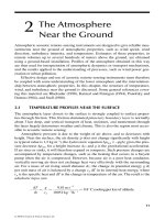
This chapter provides an overview of existing and planned satellite-based
systems subdivided into the categories of high spatial resolution systems, high
spectral resolution systems, high temporal resolution systems and radar systems
(Figure 3.1). More technical details of some of these systems can be found in
Kramer (1996). For readers requiring details of existing remote sensing systems as
well as historical image archives, please refer to the references and internet links
provided at the end of the chapter. The different sensor systems are catalogued
within the internet links provided according to the order in which they are treated in
the text.
A
brief discussion on the various application fields for the sensor types
will follow the technical description of the instruments. The chapter provides a few
classical references that serve as a starting point for further studies without
Copyright 2002 Andrew Skidmore
New environmental remote sen.ring systems
27
attempting to be complete. In addition, cross references to other chapters in this
book serve as a basis for a better understanding of the diversity of applications.
Swath width
(km)
Figure 3.1:
Classification

of
sensors.
3.2
HIGH SPATIAL RESOLUTION SENSORS
3.2.1
Historical overview
High spatial resolution sensors have a resolution of less than
5
m and were once the
exclusive domain of spy satellites. In the
1960s, spy satellites existed that had a
resolution better than 10 meters. Civil satellites had to wait until the very last days
of the
2oth century. The major breakthrough was one of policy rather than
technology. The US Land Remote Sensing Act of 1992 concluded that a robust
commercial satellite remote-sensing industry was important to the welfare of the
USA and created a process for licensing private companies to develop, own,
operate, and sell high-resolution data from Earth-observing satellites. Two years
later four licences for one-meter systems were granted, and currently the first
satellite, IKONOS, is in space. This innovation promises to set off an explosion in
the amount and use of high resolution image data.
High-resolution imaging requires a change in instrument design to a
pushbroom and large telescope, as well as a new spacecraft design. In contrast to
the medium-resolution satellites, high-resolution systems have limited multispectral
coverage, or even just panchromatic capabilities. They do have extreme pointing
capabilities to increase their potential coverage. The pointing capability can also be
used for last minute reprogramming of the satellite in case of cloud cover.
The private sector has shown an almost exclusive interest in high-resolution
systems. Obviously, it is believed that these systems represent the space capability
needed to create commercially valuable products. On the other hand, pure

commercial remote sensing systems, with no government funding, implies a high
Copyright 2002 Andrew Skidmore
28
Environmental Modelling with GIS and Remote Sensing
risk, especially to data users. Most companies in the high-resolution business have
a back-up satellite in store, in order to be able to launch a replacement satellite at
short notice. But still, the loss of one satellite means a loss of millions of dollars,
which may be considerable for a business just starting in this field. The
characteristics of high-resolution satellites include a spatial resolution of less than 5
m, 1 to
4
spectral bands, a swath less than 100
km
and a revisiting time of better
than 3 days.
3.2.2 Overview sensors
An overview of high-resolution sensors to be discussed is given in Table 3.1.
Table
3.1:
Typical high-resolution satellites.
Platform Sensor Spatial Multi- Swath Pointing Revisit
resolution spectral width capability time
IRS- PAN 5.8 m 4 bands 70 km
f26" 5 days
IC&D*
Cosmos* KVR-1000 -2 m No 160km No N/A
OrbView-3 PAN
I
m 4 bands
8

km 1-45" 3 days
Ikonos 1 OSA I m 4 bands I l km ?30° 1-3 days
QuickBird QBP I m
4
bands 27 km 1-30" 1-3 days
EROS A+ CCD 1.8 m No 12.5 km
3.2.3
IRS-1C
and
IRS-1D
Having been the seventh nation to successfully launch an orbiting remote sensing
satellite in July 1980, India is pressing ahead with an impressive national
programme aimed at developing launchers as well as nationally produced
communications, meteorological and Earth resources satellites. The IRS-
1C and 1D
offer improved spatial and spectral resolution over the previous versions of the
satellite, as well as on-board recording, stereo viewing capability and more frequent
revisits. They carry three separate imaging sensors, the WiFS, the LISS, and the
high-resolution panchromatic sensor.
The Wide Field Sensor (WiFS) provides regional imagery acquiring data with
800
km
swaths at a coarse 188 m resolution in two spectral bands, visible (620-680
nm) and near infrared (770-860 nm), and is used for vegetation index mapping. The
WiFS offers a rapid revisit time of 3 days.
The Linear Imaging Self-scanning Sensor 3 (LISS-3) serves the needs of
multispectral imagery clients, possibly the largest of all current data user groups.
LISS-3 acquires four bands (520-590, 620-680, 770-860, and 1550-1750 nm) with
*
IRS-I, Pan and Cosmos do not meet the strict definition of 'high resolution imagery', but is

considered to be an example of this genre.
Copyright 2002 Andrew Skidmore
New environmental remote sensing systems
29
a 23.7 m spatial resolution, which makes it an ideal complement to data from the
aging
Landsat 5 Thematic Mapper
(TM)
sensor.
The most interesting of the three sensors is the panchromatic sensor with a
resolution of 5.8 m. With its 5.8 m resolution, the
IRS-1C and IRS-1D can cover
applications that require spatial detail and scene sizes between the 10 m SPOT
satellites and the
1 m systems. The PAN sensor is steerable up to plus or minus 26
degrees and thus offers stereo capabilities and a possible frequent revisit of about 5
days, depending on the latitude. Working together, the
IRS-1C and ID will also
cater to users who need a rapid revisiting rate.
IRS-1C was launched on 28
December 1995,
IRS-1D on 28 September 1997. Both sensors have a 817
km
orbit,
are sun-synchronous with a
10:30 equator crossing, and a 24-day repeat cycle.
India will initiate a high-resolution mapping programme with the launch of
the
IRS-P5, which has been dubbed Cartosat-I. It will acquire 2.5 m resolution
panchromatic imagery. There seem to be plans to futher improve the planned

Cartosat-2 satellite to achieve 1 m resolution.
Data from the Russian KVR-1000 camera, flown on a Russian Cosmos satellite, is
marketed under the name of SPIN-2 (Space Information
-
2 m). It provides high-
resolution photography of the USA in accordance with a Russian-American
contract. Currently SPIN-2 offers some of the world's highest resolution,
commercially available satellite imagery. SPIN-2 panchromatic imagery has a
resolution of about 2 m. The data is single band with a spectral range between 5 10
and 760 nm. Individual scenes cover a large area of 40
km
by 180
km.
Typically,
the satellite is launched and takes images for 45 days, before it runs out of fresh
film; the last mission was in February-March 1998. The KVR-1000 is in a
low-
earth orbit and provides 40
x
160
km
scenes with a resolution.
OrbView-3 will produce 1 m resolution panchromatic and 4 m resolution
multispectral imagery.
OrbView-3 is in a 470
km
sun-synchronous orbit with a
10:30 equator crossing. The spatial resolution is 1 m for a swath of 8 km and a 3
day revisit time. The panchromatic channel covers the spectral range from 450 nm
to 900 nm. The four multispectral channels cover 450-520 nm, 520-600 nm,

625-695 nm, and 760-900 nm respectively. The design lifetime of the satellite is
5
years. In Europe, Spot Image will have the exclusive right to sell the imagery of
OrbImage's planned OrbView-3 and OrbView-4 satellites. OrbView-3 and
OrbView 4 are planned to be launched in 2001.
3.2.6
Ikonos
The Ikonos satellite system was initiated as the Commercial Remote Sensing
System (CRSS). The satellite will routinely collect 1 m panchromatic and 4 m
Copyright 2002 Andrew Skidmore
30
Environmental Modelling with CIS and Remote Sensing
multispectral imagery. Mapping North America's largest 100 cities is an early
priority. The sensor OSA (Optical Sensor Assembly) features a telescope with a 10
m focal length (folded optics design) and pushbroom detector technology.
Simultaneous imaging in the panchromatic and multispectral modes is provided. A
body pointing technique of the entire spacecraft permits a pointing capability of
?3O0 in any direction. Ikonos is in a 680
km,
98.2", sun-synchronous orbit with a
14 days repeat cycle and a 1-3 day revisit time. The sensor has a panchromatic
spectral band with 1 m resolution (0.45-0.90) and 4 multispectral bands
(0.45-0.52,
0.52-0.60,0.63-0.69, 0.76-0.90) with 4 m resolution. The swath is 11
km.
3.2.7
QuickBird
QuickBird is the next-generation satellite of the EarlyBird satellite. Unfortunately,
EarlyBird was lost shortly after launch in December 1997. Its follow-up QuickBird
(QuickBird-1 was launched on 20 November 2000, and also failed). The system

has a planed panchromatic channel (0.45-0.90) with 1 m resolution at nadir and
four multispectral channels
(0.45-0.52,0.53-0.59, 0.63-0.69, 0.77-0.90) with 4 m
resolution.
3.2.8
Eros
Eros (12.5 km swath) is the result of a joint venture between the US and Israel. The
Eros A+ satellite will have a resolution of about 1.8 m. The follow-up satellite Eros
B will have a resolution of about 80 cm.
EROS satellites are light, low earth orbiting, high resolution satellites. There
are two classes of EROS satellite, A and B. EROS
A1 and A2 will weigh 240 kg at
launch and orbit at an altitude of 480 km. They will each carry a camera with a
focal plane of CCD (Charge Coupled Device) detectors with more than 7,000
pixels per line. The expected lifetime of EROS A satellites is at least 4 years.
EROS B 1-B6 will weigh under 350 kg at launch and orbit at an altitude of 600 km.
They carry a camera with a
CCDITDI (Charge Coupled DeviceITime Delay
Integration) focal plane that enables imaging even under weak lighting conditions.
The camera system provides 20,000 pixels per line and produces an image
resolution of 0.82 m. The expected lifetime of EROS B satellites is at least 6 years.
EROS satellites will be placed in a polar orbit. Both satellites are sun-
synchronous. The light, innovative design of the EROS satellites allows for a great
degree of platform agility. Satellites can turn up to 45 degrees in any direction as
they orbit, providing the power to take shots of many different areas during the
same pass. The satellites' ability to point and shoot their cameras also allows for
stereo imaging during the same orbit. The satellites will be launched using
refurbished Russian ICBM rocket technology, now called Start-1. Satellites will be
launched from 2000-2005;
EROS-A1 was launched on 5 December 2000.

Copyright 2002 Andrew Skidmore
New environmental remote sensing systems
3.2.9
Applications and perspectives
Satellite images have traditionally been used for military surveillance, to search for
oil and mineral deposits, infrastructure mapping, urban planning, forestry,
agriculture and conservation research. Agricultural applications may benefit from
the increased resolution. The health of agricultural crops can be monitored by
analyzing images of near-infrared radiation. Known as 'precision agriculture',
farmers are able to compare images one or two days apart and apply water,
fertilizer or pesticides to specific areas of a field, based on coordinates from the
satellite image, and a Global Positioning System (GPS). In forestry, individual trees
could be identified and mapped over large areas (see Chapter 6 by Woodcock
et
al.).
Geographic information systems (GIs) databases may be constructed using 1
m images, reducing reliance on out-of-date paper maps. Highly accurate elevation
maps (or Digital Elevation Models
-
DEMs), may be also be developed from the
images and added to the databases. Because they cover large areas, high-resolution
satellite images could replace aerial photographs for certain types of detailed
mapping; for example, gas pipeline routing, urban planning and real estate. This
includes the use of high resolution imagery for three-dimensional drapes that can be
used to visualize and simulate land-management activities.
3.3
HIGH
SPECTRAL RESOLUTION SATELLITES
3.3.1
Historical overview

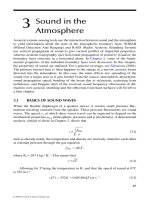
Imaging spectrometry satellites use a near-continuous radiance or reflectance to
capture all spectral information over the spectral range of the sensor. Imaging
spectrometers typically acquire images in a large number of channels (over
40),
which are narrow (typically 10 to 20 nm in width) and contiguous (i.e., adjacent
and not overlapping
-
see Figure 3.2). The resulting reflectance spectra, at a pixel
scale, can be directly compared with similar spectra measured in the field, or
laboratory. This capability promises to make possible entirely new applications and
to improve the accuracy of current multispectral analysis techniques. The demand
for imaging spectrometers has a long history in the geophysical field; aircraft-based
experiments have shown that measurements of the continuous spectrum allow
greatly improved mineral identification (Van der Meer and Bakker 1997). The first
civilian airborne spectrometer data were collected in 1981 using a one-dimensional
profile spectrometer developed by the Geophysical Environmental Research
Company. These data comprised 576 channels covering the 4 to 2.5
pm wavelength
range (Chiu and Collins 1978). The first imaging device was the Fluorescence Line
Imager
(FLI; also known as the Programmable Line Imager, PMI) developed by
Canada's Department of Fisheries and Oceans in 1981. The Airborne Imaging
Spectrometer (AIS), developed at the NASA Jet Propulsion Laboratory was
operational from 1983 onward. This instrument acquired data in 128 spectral bands
in the range of 1.2-2.4 ym. with a field-of-view of 3.7 degrees resulting in images
of 32 pixels width (Vane and Goetz 1988). A later version of the instrument, AIS-
2, covered the 0.8-2.4
pm region acquiring images 64 pixels wide (LaBaw 1987).
In 1987 NASA began operating the Airborne
VisibleIInfrared Imaging

Copyright 2002 Andrew Skidmore
32
Environmental Modelling with GIs and Remote Sensing
Spectrometer (AVIRIS; Vane
et
al.
1993).
AVIRIS was developed as a facility that
would routinely supply well-calibrated data for many different purposes. The
AVIRIS scanner simultaneously collects images in
224
contiguous bands resulting
in a complete reflectance spectrum for each
20
by
20
m. pixel in the
0.4
to
2.5
pm
region with a sampling interval of
10
nm (Goetz
et
al.
1983;
Vane and Goetz
1993).
The field-of-view of the AVIRIS scanner is

30
degrees resulting in a ground
field-of-view of
10.5km.
Private companies now recognize the potential of imaging
spectrometry and have built several sensors for specific applications. Examples are
the GER imaging spectrometer (operational in
1986),
and the ITRES CASI that
became operational in
1989.
Currently operational airborne instruments include the
NASA instruments (AVIRIS, TIMS and MASTER), the DAIS instrument operated
by the German remote sensing agency DLR, as well as private companies such as
HyVISTA who operate the HyMAP scanner or the Probe series of instruments
operated by Earth Search Sciences, Inc.
Imaging Spectroscopy is the acquisition of images where for each spatial
resolution element in the image a spectrum of the energy arriving at the sensor
is
measured. These spectra are used to derive information based on the signature of
the interaction of matter and energy expressed in the spectrum. This spectroscopic
approach has been used in the laboratory and in astronomy for more than
100
years, but is a relatively new application when images are formed from aircraft or
spacecraft.
each oixel has an
assoctated, continuous
spectrum that can be
Figure
3.2:

Concept of
imaging
spectroscopy.
Copyright 2002 Andrew Skidmore
New environmental remote sensing sysrems
33
3.3.2
Overview hyperspectral imaging sensors
An overview of imaging spectrometry sensors that are discussed here is given in
Table 3.2.
Table
3.2:
Some imaging spectrometry satellites.
Platform Sensor Spatial Spectral Spectral Swath Revisit
resolution bands range
(pn)
width time
ENVISAT-1 MERIS 300
rn
15
EOS-AM1 ASTER 15-90
rn
14 0.52-1 1.65 60
km
Orbview 4
8rn
200 0.45-2.5 5
km
3
days

NMPIEO-
1
Hyperion
30
rn
220 0.4-2.5 7.5
LAC 250
rn
256 0.9-1.6 185
krn
Aries-
1
30
rn
64 0.4-1.1 15
km
7
days
The European Space Agency (ESA) is developing two spaceborne imaging
spectrometers: The Medium Resolution Imaging Spectrometer (MERIS) and the
High Resolution Imaging Spectrometer (HRIS); now renamed to PRISM, the
Process Research by an Imaging Space Mission (Posselt
et
al.
1996). MERIS,
currently planned as payload for the satellite
Envisat-1 to be launched in 2002, is
designed mainly for oceanographic application and covers the 0.39-1.04
ym
wavelength region with 1.25 nm bands at a spatial resolution of 300 m or 1200 m.

(Rast and Bezy 1995). PRISM, currently planned for Envisat-2 to be launched
around the year 2003, will cover the 0.4-2.4
pm wavelength range with a 10 nm
contiguous sampling interval at a 32 m ground resolution.
The EOS (Earth Observing System) is the centerpiece of NASA's Earth Science
mission. The EOS AM-1 satellite, later renamed to Terra, is the main platform that
was launched on 18 December 1999. It carries five remote sensing instruments
(including
MODIS and ASTER). EOS-AM1 orbits at 705 km, is sun-synchronous
with a
10:30 equator crossing and a repeat cycle of 16 days. ASTER (the Advanced
Spaceborne Thermal Emission and Reflectance Radiometer) has three bands in the
visible and near-infrared spectral range with a 15 m spatial resolution, six bands in
the short wave infrared with a 30 m spatial resolution, and five bands in the thermal
infrared with a 90 m spatial resolution. The VNIR and SWIR bands have a spectral
resolution in the order of 10 nm. Simultaneously, a single band in the near-infrared
will be provided along track for stereo capability. The swath width of an image will
be 60
km
with 136
km
crosstrack and a temporal resolution of less than 16 days.
Also on the
EOS-AM1, the Moderate resolution imaging spectroradiometer
(MODIS) is planned as a land remote sensing instrument with high revisting time.
MODIS is mainly designed for global change research (Justice
et
al.,
1998).
Copyright 2002 Andrew Skidmore

34
Environmental Modelling with CIS and Remote Sensing
ASTER carries three telescopes: VNIR 0.56, 0.66, 0.81
pm;
SWIR 1.65, 2.17,
2.21, 2.26, 2.33, 2.40
ym; TIR 8.3, 8.65, 9.10, 10.6, 11.30 ym with spatial
resolutions of VNIR
15 m, SWIR 30 m, TIR 90 m.
OrbView-4 will be the successor of the OrbView-3 high-resolution satellite. As
with
OrbView-3, OrbView-4's high-resolution camera will acquire 1 m resolution
panchromatic and 4 m resolution multispectral imagery. In addition,
OrbView-4
will acquire hyperspectral imagery. The sensor will cover the 450 to 2500 nm
spectral range with 8 m nominal resolution and a 10 nm spectral resolution in 200
spectral bands. The data available to the public will be resampled to 24 m. The 8 m
data will only be used for military purposes. OrbView-4 will be launched on 31
March 2001. The satellite will revisit each location on Earth in less than three days
with an ability to turn from side-to-side up to 45 degrees from a polar orbital path.
NASA's New Millennium Program Earth Observer 1
(NMPIEO-1; see Table 3.3)
is an experimental satellite carrying three advanced instruments as a technology
demonstration (EO-1 is now called Earth Observing-1). It carries the Advanced
Land Imager
(ALI),
which will be used in conjunction with the ETM+ sensor (see
Landsat
7
below for a comparison of the two sensors). Next to the multispectral

instrument it carries two hyperspectral instruments, the
Hyperion and the LEISA
Atmospheric Corrector (LAC). The focus of the
Hyperion instrument is to provide
high-quality calibrated data that can support the evaluation of hyperspectral
technology for spaceborne Earth observing missions. It provides hyperspectral
imagery in the 0.4 to 2.5 ym region at continuous 10 nm intervals. Spatial
resolution will be 30 m. The LAC is intended to correct mainly for water vapour
variations in the atmosphere using the information in the 890 to 1600 nm region at
2 to 6 nm intervals. In addition to atmospheric monitoring, LAC will also image the
Earth at a spatial resolution of 250 m. The imaging data will be cross-referenced to
the
Hyperion data where the footprints overlap.
The EO-1 was successfully
launched on 21 November 2000.
Table 3.3: Characteristics
of
EO-1.
Hyperion
LAC
Spectral range 0.4-2.5 m
0.9-1.6 m
Spatial resolution
30 m 250 m
Swath width
7.5
km
185 km
Spectral resolution
10 nm 2-6 nm

Spectral coverage continuous continuous
Number of bands
220 256
Copyright 2002 Andrew Skidmore
New environmental remote sensing systems
Aries-1 is a purely Australian initiative to build a hyperspectral satellite, mainly
targeted at geological applications for the (Australian) mining business. The
ARIES-1 will be operated from a 500
krn
sun-synchronous orbit. The system will
have a VNIR and SWIR hyperspectral, and
PAN
band setting with 128 bands in the
0.4
-
1.1 ym and 2.0
-
2.5
ym regions. The
PAN
band will have 10 m resolution,
the hyperspectral bands will have 30 m resolution. The swath width is 15 km with a
revisit time of
7
days.
3.3.3
Applications and perspectives
The objective of imaging spectrometry is to measure quantitatively the components
of the Earth from calibrated spectra acquired as images for scientific research and
applications. In other words, imaging spectrometry will measure physical quantities

at the Earth's surface such as upwelling radiance, emissivity, temperature and
reflectance. Based upon the molecular absorptions and constituent scattering
characteristics expressed in the spectrum, the following objectives will be
researched and solution found to:
Detect and identify the surface and atmospheric constituents present
Assess and measure the expressed constituent concentrations
Assign proportions to constituents in mixed spatial elements
Delineate spatial distribution of the constituents
Monitor changes in constituents through periodic data acquisitions
Simulate, calibrate and intercompare sensors.
Through measurement of the solar reflected spectrum, a wide range of scientific
research and application is being pursed using signatures of energy, molecules and
scatterers in the spectra measured by imaging spectrometers. Atmospheric science
includes the use of hyperspectral sensors for the prediction of various constituents
such as gases and water vapour. In ecology, some use has been made of the data for
quantifying photosynthetic and non-photsynthetic constituents. In geology and soil
science, the emphasis has been on mineral mapping to guide in mineral
prospecting. Water quality studies have been the focus of coastal zone studies.
Snow cover fraction and snow grain size can be derived from hyperspectral data.
Review papers on geological applications can be found in van der Meer (1999).
Cloutis (1996) provides a review of analytical techniques in imaging spectrometry
while Van der Meer (2000) provides a general review of imaging spectrometry.
Clevers (1999) provides a review of applications of imaging spectrometry in
agriculture and vegetation sciences.
Copyright 2002 Andrew Skidmore
36
Environmental Modelling with
GIS
and Remote Sensing
3.4 HIGH TEMPORAL RESOLUTION SATELLITES

3.4.1 Low spatial resolution satellite systems with high revisiting time
Typically, these satellites (Table 3.4) have a spatial resolution larger than 100 m.
They trade reduced spatial and spectral resolution against high frequency visits. A
global system of geo-stationary and polar orbiting satellites is used to observe
global weather. Other satellites are used for oceanography, and for mapping
phenomena on a continental or even global scale. Typical low-resolution satellite
systems have a spatial resolution of 100 m or lower, few (3-7) spectral bands, large
(>500
km)
swath width and daily revisit capability.
Table
3.4:
A
selection of low-resolution satellites with high revisiting time.
Platform Orbit Sensor Spatial Spectral Swath Revisit
resolution bands width time
Meteosat
GEO
VISSR
2.5
km
3
Earth Disc
30
min
NO A A Polar AVHRR 1
7
3000
km
Daily

Resurs-Ol Sun-sync MSU-SKI
200-300
rn
4
760
km
3-5
days
SeaStar
Sun-sync
SeaWiFS 1.1
km
8
2800
km
Daily
3.4.1.1 Meteosat
Meteosat 1 was the first European meteorological geo-stationary satellite. Meteosat
5
is currently the primary satellite, with Meteosat 6 as standby. Meteosat is
controlled by Eumetsat, an international organization representing 17 European
states. Meteosat Second Generation (MSG) will appear in the year 2000, together
with the first polar orbiting
Metop satellite. Meteosat is in a geo-stationary orbit at
0" longitude. The sensor has spectral bands at 0.5-0.9 pm (VIS), 5.7-7.1 pm
(WV), and 10.5-12.5 pm (TIR) with spatial resolutions of 2.5 km VIS and WV and
5 km TIR. The revisit time is 30 minutes.
3.4.1.2
NOAA
The NOAA satellite program, designed primarily for meteorological applications,

has evolved over several generations of satellites (TIROS, ESSA, TIROS-M, and
TIROS-N, to NOAA-KLM series), starting with TIROS-1 through to the most
recent NOAA-15. These satellites have provided different instruments for
measuring the atmosphere's temperature and humidity profiles, the Earth's
radiation budget, space environment, instruments for distress signal detection
(search and rescue), instruments for relaying data from ground-based and airborne
stations, and more.
For Earth observation the most interesting instrument is the Advanced Very
High Resolution Radiometer (AVHRR) scanner. The AVHRR scans the Earth in
five spectral bands: band 1 in the visible red around 0.6
pm, band 2 in the near
infrared around 0.9
pm, band 3 in the mid-wave infrared around 3.7 pm, and band
4 and
5
in the thermal infrared around 11 and 12 pm respectively. This
combination of bands makes the AVHRR suitable for a wide range of applications,
Copyright 2002 Andrew Skidmore
New environmental remote sensing systems
37
from measurement of cloud cover, to sea surface temperature, vegetation, land and
sea ice. The disadvantage of the AVHRR is its coarse resolution of about 1
km
at
nadir. But the major benefit of the AVHRR lies in its high temporal frequency of
coverage.
The NOAA satellites are operated in a two-satellite system. Both satellites are
in a sun-synchronous orbit, one satellite will always pass around noon and
midnight, the other always passing in the morning and in the evening. The AVHRR
sensors have an extreme field of view of

1 lo0, and together they give a global
coverage each day! Every spot on Earth is imaged at least twice each day,
depending on latitude. It is
the
instrument for observation of phenomena on a
global scale. Owing to its frequent revisit time, it is being used for many monitoring
projects on a regional scale.
The imagery of the AVHRR is also known by other names. The HRPT (High
Resolution Picture Transmission) is the digital real-time reception of the imagery
by a ground station. There are over 500 HRPT receiving stations registered by the
World Meteorological Organization (WMO) worldwide. The satellite can also be
programmed to record a number of images. Such images, although having the same
characteristics as HRPT, are called LAC (Local Area Coverage). Next to the 1
km
resolution LAC, the satellite can resample the data on the fly to 4 km resolution
GAC (Global Area Coverage). Finally, two bands of 4 km resolution imagery are
transmitted by an analogue weather fax signal from the satellite, which can be
received by relatively simple and low-cost equipment. This is called the APT
(Automatic Picture Transmission). Two excellent sources of information on NOAA
are Cracknell (1997) and
D'Souza
et
al.
(1996).
NOAA-14 (since 30
Dec 1994) and NOAA-15 (since 13 May 1998) are in a
850
km,
98.9", sun-synchronous (afternoon or morning) orbit. The spatial
resolution is

1
km
at nadir, 6
km
at limb of sensor. Spectral bands include band 1 at
580-680 nm, band 2 at 725-1 100 nm, band 3 at 3.55-3.93
pm, band 4 at 10.3-1 1.3
pm and band 5 at 11.4-12.4 pm. The revisit time is 2-14 times per day, depending
on latitude. NOAA-16 was launched on
21
September 2000.
Launched on 10 July 1998, the
Resurs-Ol#4 is the fourth operational remote
sensing satellite in the Russian
Resurs-01 series. Maybe it is not altogether fair to
list the Russian Resurs under the low-resolution category as
it
is actually equivalent
to the US
Landsat. But the satellite is best known for its relatively cheap large
coverage images of the MSU-SK conical scanner. There are only two receiving
stations located in Russia and in Sweden. The Swedish Space Corporation
Satellitbild also processes and distributes the images. With a swath of 760
km
and
resolution of about 250 m Resurs fills the gap between the
1
km
resolution NOAA
images and the 30 m resolution

Landsat images. Resurs-01 is in a 835
km,
98.75",
sun-synchronous orbit. The sensor has spectral bands at 0.5-0.6 pm, 0.6-0.7 pm,
0.7-0.8
pm, 0.8-1.1
pm
and 10.4-12.6 pm with a 30 m (MSU-E) and 200-300 m
(MSU-SK) spatial resolution. The swath width is 760
km
with a 3-5 day revisit
time.
Copyright 2002 Andrew Skidmore
38
Environmental Modelling
with
CIS and Remote Sensing
3.4.1.4
OrbView-2, a.k.a. SeaStar/Sea WiFS
Launched on 1 August 1997, SeaStar delivers multispectral ocean-colour data to
NASA until 2002. This is the first time that the US Government has purchased
global environmental data from a privately designed and operated remote sensing
satellite. SeaStar carries the SeaWiFS Sea-viewing Wide Field Sensor, which is a
next generation of the Nimbus 7's Coastal Zone Color Scanner (CZCS). SeaWiFS
measures ocean surface-level productivity of phytoplankton and chlorophyll.
However, SeaStar was originally designed for ocean colour but later changed to be
able also to measure the higher radiances from land. Thus, it provides a more
environmentally stable vegetation index than the one derived from
NOAA's
AVHRR, which is inaccurate under hazy atmospheric conditions because of its

single visible and near infrared channels. Band
1
looks at gelbstoffe, bands 2 and 4
at chlorophyll, band 3 at pigment, band 5 at suspended sediments. Bands 6,7 and 8
look at atmospheric aerosols, and are provided for atmospheric corrections.
Orbview-2 is in a 705
km,
98.2", sun-synchronous, equator crossing (at noon)
orbit. The spatial resolution of the data is 1.1 km, the swath width is 2800 km with
a 1 day revisit time. Spectral bands of the system include: 402-422 nm, 433-453
nm, 480-500 nm, 500-520 nm, 545-565 nm, 660-680 nm, 745-785 nm, 845-885
nm.
3.4.2
Medium spatial resolution satellite systems with high revisiting time
These satellites (Table 3.5) all have medium area coverage, a medium spatial
resolution, a moderate revisit capability, and multispectral bands characteristic of
the current
Landsat and Spot satellites. The scale of the images of these satellites
makes them especially suited for land management and land-use planning for
extended areas (regions, countries, continents). Most of these medium-resolution
satellites are in a sun-synchronous orbit.
Characteristics of medium-resolution and satellites with high revisiting time
include:
Spatial resolution between 10 m and 100
m
3 to 7 spectral bands
Swath between 50
km
and 200
km

Incidence angles
Revisit 3 days and more.
Copyright 2002 Andrew Skidmore
New environmental remote sensing systems
39
Table
3.5:
Some medium-resolution satellites.
Platform Sensor Spatial Spectral Swath Pointing Revisit
resolution bands width capability time
Landsat
4&5
TM
30 m 7 185 km No 16
davs
Landsat
7
ETM+
15 m (PAN) 8 185 km No 16
davs
S~ot 1-3 HRV lOm(PAN\ 3 60 km 227" 4-6
davs
Spot 4 HRVIR 10 m (PAN) 4 60 km f 27" 4-6
days
Resource2 1
M
10 I0 m (PAN) 6 205 km i30° 3-4
days
Earth observation is often associated with the Landsat satellites, having been in
operation since 1972, while

Landsat 5 has been in operation for 15 years! The
Landsat satellites were developed in the 1960s. Landsats 1, 2 and 3 were enhanced
versions of the Nimbus weather and research satellites, and originally known as the
Earth Resources Technology Satellites (ERTS). The moment
Landsat 1 became
operational its images were regarded as sensational by early investigators. The
quality of the images led to the information being put to immediate practical use. It
became clear that they were directly relevant to the management of the world's
food, energy and environment. The
Landsat satellites have flown the following
sensors:
The Return Beam Vidicon (RBV) Camera
Multi-spectral Scanner (MSS)
Thematic Mapper (TM).
Landsat 4 was launched on 16 July 1982, and a failing power system on Landsat 4
prompted the launch of
Landsat 5 two years later on 1 March 1984. The loss of
Landsat
6
in October 1993 was a severe blow to the system. Both Landsat 4 and 5
suffer from degrading sub-systems and sensors and are expected to fail any
moment. At present,
Landsat 7 is in operation.
The characteristics of Landsats 4 and 5 include:
Operational: Landsat 5 (since 1 March 1984!)
Orbit: 705 km, 98.2", sun-synchronous 09:45
AM
local time equator crossing
Repeat cycle: 16 days
Sensor: Thematic Mapper (TM), electro-mechanical oscillating mirror scanner

Spatial resolution TM: 30 m (band
6:
120 m)
Spectral bands TM (pm): band 1 0.45-0.52; band 2 0.52-0.60; band 3
0.63-0.69; band 4 0.76-0.90; band 5
1.55-1.75;band
6
10.4-12.50; band 7
2.08-2.35
Field of view (FOV): 15", giving 185
km
swath width.
Copyright 2002 Andrew Skidmore
40
Environmental Modelling with GIS and Remote Sensing
Characteristics of Landsat 7 include:
Operational:
Landsat 7 Orbit: 705
km,
98.2", sun-synchronous 10
AM
local
time equator crossing
Repeat cycle: 16 days
Sensor: Enhanced Thematic Mapper+
(ETM+), electro-mechanical oscillating
mirror scanner; imagery can be collected in low- or high-gain modes; high gain
doubles the sensitivity
Spatial resolution: 30 m (PAN: 15 m, band 6: 60 m)
Spectral bands

(pm): band 1 0.45-0.52; band 2 0.52-0.60; band 3 0.63-0.69;
band 4 0.76-0.90; band 5 1.55-1.75; band 6 10.4-12.50; band 7 2.08-2.35;
band 8 (PAN) 0.50-0.90
Field of view (FOV):
15", 185
km
Downlink: X-band, 2x150 Mbit/s, 300 Mbit/s playback
Onboard recorder: 375 Gbit Solid State Recorder for about 100 ETM+ scenes.
3.4.2.2
SPOT
1/2/3
(Systkme Pour I'Obsewation de la Terre)
First named Systkme Probatoire d70bservation de la Terre (Test System for Earth
Observation), but later renamed to
Systkme Pour l'observation de la Terre (System
for Earth Observation), the Spot system has been in operation since 1986. The Spot
satellites each carry two identical
HRV (High-Resolution Visible) sensors,
consisting of CCD (Charge-Coupled Device) linear arrays. Essentially, all the
points of one line are imaged at the same time by the many detectors of the linear
array. The Spot sensors can be tilted from the normal downward viewing mode by
plus or minus 27 degrees, which offers the possibility to view objects from two
different sides. These stereo images can be used to determine the height of objects,
or even the height of the terrain. Spot 1 was already put in standby mode, but
reactivated after Spot 3 failed on 14 November 1996. Spot 3 ran out of power when
an incorrect series of commands was sent to the satellite, and could not be
recovered. An important addition to Spot 4 is the VEGETATION instrument. With
resolution of 1.15
km
at nadir, and a swath width of 2,250 kilometers, the

VEGETATION instrument will cover almost all of the globe's landmasses while
orbiting the Earth 14 times a day. Characteristics of Spot
11213 include:
Orbit: 832
km,
98.7", sun-synchronous 10:30
AM
local time equator crossing
Repeat cycle: 26 days
Sensor:
2xHRV
(High Resolution Visible), pushbroom linear CCD array
Spatial resolution: MS mode 20 m,
PAN
10 m
Spectral bands MS (nm): band 1 500-590; band 2 610-680; band 3 790-890
Panchromatic mode: 5 10-730 nm
Swath width: 60
km
Steerable:
f
27" left and right from nadir
Of-nadir Revisit time: 4-6 days.
Copyright 2002 Andrew Skidmore
New environmental remote sensing systems
41
Characteristics of Spot 4 include:
Orbit: same as SPOT 1-2-3
Sensors: 2xHRVIR (High-Resolution Visible and Infrared), pushbroom linear
CCD array, VEGETATION

Spatial resolution: MS mode 20 m, PAN 10 m, VEGETATION 1.15
km
Spectral bands MS (nm): band 1 500-590; band 2 610-680; band 3 790-890;
band 4
1.58-1.75 ym
Panchromatic mode: 610-680 nm (same as MS band 2!)
VEGETATION bands: band 1 0.43, bands 21314 same as HRVIR
VEGETATION swath: 2250
km.
Resource21 is the name of a commercial remote sensing information services and
services company based in the US. Resource21 will combine satellite and aircraft
remote sensing to provide twice-weekly information products within hours of data
collection, based on 10 m resolution multispectral. The complete system will
consist of four satellites. All areas on Earth will be visited by one of the satellites
every three or four days, resulting in a revisit twice a week. In other words, the
constellation will give a global coverage every three or four days at 10 m
resolution. The main application areas of Resource21 are agriculture ('precision
farming'), and environment and natural resource monitoring.
Resource21 is at a 740
km,
98.6", sun-synchronous, 10:30 crossing at
ascending node orbit. The sensor has spectral bands (ym) at 0.45-0.52 blue,
0.53-0.59 green, 0.63-0.69 red, 0.76-0.90 NIR, 1.55-1.68 SWIR, and 1.23-1.53
cirrus clouds with a 10 m resolution in the VNIR, a 20 m resolution in the SWIR,
and a 100
m+
resolution for the cirrus band. The swath width is 205
km
with a 3-4
day revisit time. The status of the Resource21 programme is unclear. It has been on

hold for some time because of budget considerations, but Boeing continues to work
towards a realization of the programme.
3.5
RADAR
3.5.1 Historical overview
RADAR (Radio Detection And Ranging) remote sensing has been used
operationally since the 1960s. The technique uses the microwave and radio part of
the spectrum, with frequencies between 0.3
GHz and 300 GHz roughly
corresponding to wavelengths between 1 mm and 1 m, with wavelengths between
0.5 and 50 cm being widely utilized. Table 3.6 summarizes the available
wavelengths, their usage and the availability in terms of sensors.
Copyright 2002 Andrew Skidmore
Environmental Modelling with
CIS
and Remote Sensing
Table
3.6:
Radar bands used in Earth observation, with corresponding frequencies.
Sources: Hoekrnan
(1990)
and van der Sanden
(1997).
Band Frequency
(GHz)
Available in
Ka 35.5
-
35.6 Airborne sensors
K 24.05

-
24.25 Airborne sensors
Ku 17.2
-
17.3 Airborne sensors
Ku 13.4
-
14.0 Airborne sensors
X
9.50
-
9.80 Airborne sensors
X
8.55
-
8.65 Airborne sensors
C
5.25
-
5.35 Airborne sensors, ERS-
I,
-2, RADARSAT
S 3.1 -3.3 ALMAZ
L
1.215
-
1.3 Airborne sensors, SEASAT, JERS-
1
(out
of

use)
P 0.44 (central frequency) Airborne sensors
The first airborne systems were called SLAR (Side Looking Airborne Radar), as
the instrument looked at an area that was not directly under, but on one side of, an
aircraft. These radar systems are also called RAR (Real Aperture Radar), as the real
length of the antenna was used (Hussin
et
al.
1999).
Further technical developments made it possible to increase the antenna
length virtually by using the Doppler effect. These systems are called SAR
(Synthetic Aperture Radar). This new technique made it possible to increase the
spatial resolution without increasing the antenna length (with the sensor flying at
the same height) or to mount the sensor on a satellite without loosing too much of
the spatial resolution. SAK systems also look at one side of the aircraft or the
satellite, however, the term 'SLAR' is never used to describe these radar systems.
The latest development in radar technology is the so-called active phased
array antenna, presently only operational in the airborne version in the PHARUS
system (PHased AKray Universal SAR), but in future it may be also available in
spaceborne systems (i.e., the ASAR instrument of the planned ENVISAT satellite).
'I'he advantage of this system is that it is relatively small and lightweight.
Most imaging radar systems use an antenna that generates a horizontal
waveform, referred to as horizontal polarization. After backscattering from an object,
a portion of the returned energy may still retain in the same polarization as that of the
transmitted signal. However, some objects tend to depolarize (the vibration of the
wave deviates from its original direction) a portion of the microwave energy. The
portion of the signal that is depolarized is a function of surface roughness and
structural orientation. The switching mechanism in the emitting and receiving system,
alternating between two receiver or emitter channels, permits both the horizontal and
the vertical signals to be emitted or echoes to be received and recorded. The notation

HH is used to denote that the signal is horizontally emitted and the ccho horizontally
received, while HV indicates horizontal emission and vertical reception. In the same
way the notations VV and VH are used. HH and VV represent like polarization,
while HV and VH are called cross-polarization return. HV and VH tend to produce
similar results, therefore they are not used simultaneously. The like, or cross-
polarization is an important factor when considering the orientation of the ground
Copyright 2002 Andrew Skidmore
New environmental remote sensing systems
43
objects or their geometric properties, e.g. a vertical stump of a tree returns more
vertical than horizontally polarized signals.
Radar remote sensing is now used with interferometry. For example, the use
of SAR as an interferometer, the so-called SAR interferometry
(InSAR; Massonnet
et
al.,
1994), is technically difficult due to stringent requirements for stability of the
satellite orbit. Interferometry coupled with satellite SAR offers the possibility to
map the Earth's land and ice topography and to measure small displacements over
large temporal and spatial scales with subcentimeter accuracy, independent of sun
illumination and cloud coverage. Interferometric SAR makes use mainly of the
phase measurements in two or more SAR images of the same scene, acquired at
two different moments and at two slightly different locations. By interference of the
two images, very small slant range of the same surface can be inferred. These slant
range changes can be related to topography and/or surface deformations.
The most important drawback of radar images is that the reflections of radar
signals are very complex functions of the physical and structural properties, as well
as water content of the target objects. This means that the interpretation of radar
images is completely different than the interpretation of optical images.
Characteristics of radar satellites include:

Spatial resolution between 10 m to 100 m
Single or multiple (up to
3)
radar frequencies
Single or multiple polarization modes (HH, VV, HV, VH)
Wavelengthslfrequencies (see Table 3.6).
3.5.2
Overview
of
sensors
3.5.2.1 ERS-1
and
2
The European Remote Sensing (ERS 1) satellite has three primary all-weather
instruments providing systematic, repetitive global coverage of ocean, coastal
zones and polar ice caps, monitoring wave height and wavelengths, wind speed and
direction, precise altitude, ice parameters, sea surface temperature, cloud top
temperature, cloud cover, and atmospheric water vapour content. ERS-1 was
launched on 17 July 1991, it went out of service on 10 March 2000 due to a failure
of the attitude control system. ERS-2 was launched on 21 April 1995.
The Active Microwave Instrument (AMI) can operate as a wind scatterometer
or SAR. The Along-Track Scanning Radiometer
&
Microwave Sounder (ATSR-M)
provides the most accurate sea surface temperature to date. The Radar Altimeter
(RA) measures large-scale ocean and ice topography and wave heights. In addition
to these instruments, the ERS
2
also carried a Global Ozone Monitoring
Experiment

(GOME) to determine ozone and trace gases in troposphere and
stratosphere.
The ERS 2 satellite has provided continuity of data until the launch of Envisat
1. ERS 1 and 2 operated simultaneously from 15 August to May 1996, the first time
that two identical civil
SARs worked in tandem. The orbits were carefully phased
to provide 1 day revisits, allowing the collection of interferometric
SAR image
pairs and improving temporal sampling. Although still working perfectly, a lack of
funding required ERS 1 to be put on standby from May 1996.
Copyright 2002 Andrew Skidmore
44
Environmental Modelling
with
GIs
and Remote Sensing
ERS is a C-band radar system with a 100 km swath and a VV polarization.
The orbital parameters include a 771x797
km,
98.55", sun-synchronous orbit with a
168-day repeat cycle.
3.5.2.2 Radarsat
Radarsat was launched on 4 November 1995. The Boeing Company will launch
Canada's Radarsat-2 Earth-observation satellite,
synthetic aperture radar (SAR)
system in 2003. Radarsat-2, follow-on to
Radarsat-1, is a jointly funded programme
between the Canadian Space Agency (CSA) and
MacDonald Dettwiler. It is part of
a public-private sector partnership and a further step towards commercialization of

the spaceborne radar
imaging business.
Designed, constructed, launched, and operated by the CSA,
Radarsat is a
commercial radar remote sensing satellite dedicated to operational applications. Its
C-band SAR has seven different modes of 10 to 100 m resolution and 50 to 500
km
swath widths combined with 25 beam positions ranging from 10 to 60 degrees
incidence angles. Thus, a wide variety of products can be offered. The
Radarsat
system is designed to operate with no backlog, so that all imagery can be processed
and distributed within 24 hours and be available to a customer within 3 days of
acquisition.
3.5.2.3 Envisat
In 2002 the European Space Agency will launch Envisat-1, an advanced polar-
orbiting Earth observation satellite, which will provide measurements of the
atmosphere, ocean, land, and ice. Envisat-1, will be placed in a 800
km,
98.55",
orbit with a crossing at the equator at 10:OO and a 35 day repeat cycle, are a large
satellite carrying a substantial number of sensors. The most important sensors for
land applications are the Advanced Synthetic Aperture Radar (ASAR), the Medium
Resolution Imaging Spectrometer (MERIS), and the Advanced Along-Track
Scanning Radiometer (AATSR).
An ASAR, operating at C-band, ensures continuity with the image mode
(SAR) and the wave mode of the
ERS-112
AMI.
It features enhanced capability in
terms of coverage, range of incidence angles, polarization, and modes of operation.

The ERS-1 and 2 could only be switched on for 10 minutes each orbit, while the
ASAR can take up to 30 minutes of high resolution imagery each revolution.
In normal image mode the ASAR will generate high spatial resolution
products (30 m) similar to the ERS SAR. It will image one of the seven swaths
located over a range of incidence angles spanning from 15 to 45 degrees in HH or
VV polarization. As well as cross-polarization modes (HV and VH). In addition to
the 30 m resolution it offers wide swath modes, providing images of a wider strip
(405
krn)
with medium resolution (150 m). The SAR system on Envisat, AS-, is
a C-band system with HH and VV, or
HHIHV, or VVIVH modes of polarization.
The spatial resolutions are 30 m or 150 m with a swath width of 56-100 km.
Copyright 2002 Andrew Skidmore
New mvironmental remote sensing .sy.\tem.s
4
5
Together the Shuttle Imaging Radar C (SIR-C, built by JPLINASA), and the X-
band Synthetic Aperture Radar (X-SAR, jointly built by Germany and Italy) allow
radar images to be collected at 3 different wavelengths (X,
C,
and L-band) and 4
different polarization modes (HH, VV, HV, and VH). The first mission was flown
on board the Space Shuttle flight STS-59 in April 1994. The second mission was
aboard STS-68 in September-October 1994. Roughly 20 per cent of the Earth was
imaged at up to 10 m resolution. SIR-C and X-SAR have a spatial resolution of 25
m and use the X,
C,
and L-band frequencies with HH, VV, I-IV, VH, polarizations
on SIR-C and VV for X-SAR. The swath width is 15-60 km (15-45 km X-SAR).

NASA has launched the Shuttle Radar Topography Mission (SRTM;
launched on I1 February 2000) to map a digital elevation map with
16
m height
accuracy at 30
m
horizontal intervals.
SRTM
uses the SIR-C antenna working
interferometrically with additional antenna on a 60 m long deployable mast.
Approximately 80 per cent of the Earth's landmass (everything between 60" north
and 56" south latitude) will be imaged in 1000 scenes.
JERS-1 is the Japanese Earth Resources Satellite, launched on I1 February 1992.
In addition to the SAK system, it carries the OPS (Optical Sensor), which has
7
downward looking bands and one forward viewing band for stereo viewing and
uses the L-band frequency with HH polarization. The spatial resolution is 18 m at a
75 km swadth width. The original design lifetime was
2
years, but JERS-1 operated
until 1998, when a short-circuit in its solar panels immobilized it. The next
Japanese radar system will be on the ALOS (Advanced Land Observing Satellite).
ALOS will be launched in the summer of 2003.
An overview of spaceborne radar remote sensing sensors is given in Table
3.7.
Copyright 2002 Andrew Skidmore
Envzronrnentul Modelling
with
GIS
and Remote Sensing

Table
3.7:
A
selection of spaceborne radar remote sensing instruments.
Platform Sensor Spatial Frequency Polarization Swath Incidence
resolution band width angle
ERS-I&2 AMVS 30
m
C-hand VV 100
km
23"
(up
to
AR 35")
Radarsat-1 SAK 8-100
m
C-band HH 50-500 10-60"
km
Envisat-1 ASAK 30
m
C-band HH+VV, 56-100 17-45"
HWHV,
km
150
m
VVIVH 405
km
Space SIR-C 25
m
C

+
L hand HH,VV,HV, 15-60 20-55"
Shuttle VH
km
(2x ~n X-SAR X-band VV 15-45
1994)
km
JERS-I SAR 18
m
L-hand HH 75
km
35"
3.5.3
Applications
and
perspectives
Although some passive radar systems exist, using only the radiation emitted or
reflected by the Earth, most radar sensors are active sensors that emit a signal and
receive the portion of that signal that is scattered back to the sensor. Therefore,
active radar sensors are independent of solar radiation and can operate both day
and night. Because they utilize longer wavelengths, radar remote sensing is not
obstructed by clouds or by rain. Heavy rainstorms may affect the radar image,
especially if a small wavelength was used.
Radar provides information that is different from that obtained from optical
and near infrared (NIR) remote sensing. Optical/NIR remote sensing for vegetation
is based on differential scattering and absorption by the chlorophyll and leaf area,
structural characteristics and chemical composition. In contrast, the radar return
signal, or backscatter, is determined by the structure and roughness of the canopy,
the spatial distribution of the parts of the plants as well as the moisture content of
the plants, and the soil surface characteristics, such as roughness and moisture

content. The longer radar wavelengths can penetrate tree canopies and topsoil. The
use of SAR as an interferometer opens the possibility of accurate measuring of
terrain height and height differences in time leading to estimates of surface
deformation with applications in tectonics, volcanology, ice sheet mapping and so
on.
Copyright 2002 Andrew Skidmore
New environmental remote sensing systems
3.6
OTHER SYSTEMS
3.6.1 Altimetry
Altimeters use the ranging capability of radar to measure the surface topographic
profile, by simply emitting a pulse and measuring the time elapsed between
emission and reception. The height h carries a linear relationship with the time
lapse t:
h=ct/2 (Elachi, 1987). Altimeters have been flown on a number of
spacecraft, including
Seasat, ERS 1&2, and TOPEXPoseidon. Seasat produced the
first images of the
tbpography of the ocean floor, as a dip in the ocean floor causes
a dip in the water surface due to reduced gravitational pull. The ocean surface can
vary by up to 150
m. Knowing the mean water level of the oceans, minor variations
around the mean level can be measured.
TOPEXPoseidon measures ocean
temperature by these changes. There appears to be a direct relationship between
temperature and water height. The sea surface temperature reflects the temperature
in the top few centimeters of water. The sea surface measured by altimetry is
related to the temperature at all depths, as well as other parameters, such as the
water salinity and ocean currents. Note that, in general, the movement of currents
has a bigger effect on sea level

(t
1
m) than heating andor winds
(+
12 cm). All
spaceborne radar altimeters have been wide-beam systems, limited in accuracy by
their pulse duration. Such altimeters are useful for smooth surfaces (oceans),
but
are ineffective over continental terrain with relatively high relief. A fundamental
problem in narrow-beam spaceborne radar altimetry is the physical constraint of
antenna size. Again, large antennas are required for small radar footprints.
Scatterometers are radar sensors that provide the backscattering cross section of the
surface area illuminated by the sensor. They are particularly useful in measuring the
ocean backscatter in order to derive the near-surface wind vector. The strength of
the radar backscatter is proportional to the amplitude of the water surface capillary
and small gravity waves (Bragg scattering), which in turn is related to the wind
speed and direction near the surface (Elachi 1987).
3.6.3 Lidar
Lidar (LIght Detection And Ranging) refers to laser-based remote sensing. Lidar
uses principles very much like the ones used in radar. The main difference is in
wavelength; radar uses microwaves; lidar uses visible light. In fact, the term Lidar
is a generic term used for a variety of sensors operated by different concepts. Going
into detail in each of them would be beyond the scope this chapter.
The main applications of Lidar are measuring distance (height), movement,
and chemical composition. By measuring the intensity, polarization, and spectral
properties of the return signal as a function of time, one can obtain information on
the properties of the atmosphere.
Copyright 2002 Andrew Skidmore
48
Environmental Modelling with CIS and Remote Sensing

3.7 INTERNET
SOURCES
The following provides an overview of internet sources of sensors listed in this
chapter and includes sources of information for further reading.
3.7.1 High spatial resolution satellite systems
IRS:
KVR:

Orbital image (Orbview satellites):

Quickbird~Early bird:

Ikonos:

EROS:

EROS:
http:llwww.imagesatintl.coml
3.7.2 High spectral resolution satellite systems
ENVISAT:

EOS-AMlITERRA:
EOS-PMlIAqua:

Orbview-4 Orbital image (Orbview satellites):

NMPIEO-
1
:
http://eol .gsfc.nasa.gov/

ARIES:

3.7.3 High temporal resolution satellite systems
Meteosat:

NOAA (institute):
NOAA (RS data):

NOAA-POES:

Resurs:

Orbview-2 Orbital image (Orbview satellites):

SeaWifs:

Landsat-7 (at USGS):

Landat-7 (at NASA):

Landsat program:

SPOT:
http:/lwww.spotimage.fr/
3.7.4 RADAR satellite systems
ERS satellites:

Radarsat:

ENVISAT ASAR:

Copyright 2002 Andrew Skidmore
New environmental remote sensing systems
SIR:

JERS (at NASDA):
ALOS:

SRTM:

3.7.5
General sources of information
3.7.5.1 General remote sensing sites
Good points for remote sensing data sources and other related information are:
-bakkerl
3.7.5.2. Imaging spectroscopy
Spectroscopy:
http:Nspeclab.cr.usgs.gov/index.html:
Links:
~WWW/opto-knowledge/IS~resources.html
Sensor list:

3.7.5.3 RADAR remote sensing
Glossary of terminology:
http://ceo
1409.ceo.sai.jrc.it:8080/aladine/v
1.2/tutorials/glossary/agrg.html
Principle of INSAR:

Imaging radar:

Radar and radar interferometry:

.html
3.8
REFERENCES
Chiu, H.Y., and Collins, W.,
1988,
A
spectroradiometer for airborne remote
sensing.
Photogrammetric Engineering and Remote Sensing,
44:
507-5 17.
Clevers, J.G.P.W.,
1999,
The use of imaging spectrometry for agricultural
applications,
ISPRS Journal of Photogrammetry
&
Remote Sensing,
54:
299-304.
Cloutis, E.A.,
1996,
Hyperspectral remote sensing: evaluation of analytical
techniques.
Intenational Journal of Remote Sensing,
17:
2215-2242.

Cracknell, A.P.,
1997,
The advanced very high resolution radiometer AVHRR.
London,Taylor
&
Francis.
D'Souza, G., Belward, A.S., and Malingreau, J.P.,
1996,
Advances in the use of
NOAA AVHRR data for land applications.
Dordrecht, Kluwer Academic
Publishers.
Elachi, C.,
1987,
Introduction to the physics and techniques of remote sensing.
New York, Wiley
&
Sons.
Goetz,
A.F.H.,
Rowan, L.C., and Kingston, M.J.,
1983,
Mineral identification from
orbit: initial results from the Shuttle Multispectral Infrared Radiometer.
Science,
218:
1020-1031.
Copyright 2002 Andrew Skidmore
50
Environmental Modelling with

GIS
and Remote Sensing
Goetz, A.F.H., Vane, G., Solomon, J.E., and Rock, B.N., 1985, Imaging
spectrometry for earth remote sensing.
Science,
228: 1147-1 153.
Hoekman, D.H., 1990,
Radar remote sensing for applications in forestry.
PhD
thesis. Wageningen, Wageningen Agricultural University
Hussin, Y.A., Bijker, W., Hoekman, D.H., Vissers, M.A.M., and Looyen, W.,
1999,
Remote sensing applications for forest management;
workpackage report
workpackage 6; User requirement study for remote sensing based spatial
information for the sustainable management of forests. ITC, Enschede, the
Netherlands, 1999.
Justice, C.O., Vermote, E., Townshend, J.R.G., Defries, R., Roy, D.P., Hall, D.K.,
Salomonson, V.V., Privette, J.L., Riggs, G., Strahler, A., Lucht, W., Myneni,
R.B., Knyazikhin, Y., Running, S.W., Nemani, R.R., Wan,
Z.,
Huete, A.R.,van
Leeuwen, W., Wolfe, R.E., Giglio, L., Muller, J.P., Lewis, P., and Barnsley,
M.J., 1998, The Moderate Resolution Imaging Spectroradiometer
(MODIS):
Land remote sensing for global change research.
IEEE Transactions on
Geoscience and Remote Sensing,
36: 1228- 1249.
Kahle, A.B., Palluconi, F.D., Hook, S.J., Realmuto, V.J., and Bothwell, G., 1991,

The Advanced Spaceborne Thermal Emission and Reflectance Radiometer
(ASTER).
International Journal of Imaging Systems Technology,
3: 144-156.
Kramer, H. J., 1996,
Observation of the earth and its environment: survey of
missions and sensors.
Berlin, Springer-Verlag.
LaBaw, C., 1987, Airborne Imaging Spectrometer 2: The optical design, In: G.
Vane, A.F.H. Goetz
&
D.D. Norris (Eds.),
Proceedings of the Society of Photo-
optical Instrumentation Engineers,
SPIE, Vol. 834.
Massonnet, D., Feigl, K.L., Rossi, M., and Adragna, F., 1994, Radar
interferometric mapping of deformation in the year after the Landers
earthquake.
Nature,
369: 227-230.
Posselt, W., Kunkel, P., Schmidt,
E.,
Del Bello, U., and Meynart, R., 1996, Process
Research by an Imaging Space Mission. In: Fuijisada, H., Calamai, G.,
Sweeting, M. (Eds.),
Proceedings of the Advanced and Next-Generation
Satellites
I1
(SPIE, Toarmina, September 1996), Vol. 2957.
Rast, M., and

BCzy, J.L., 1995,The ESA Medium Resolution Imaging Spectrometer
(MERIS): requirements to its mission and performance of its system. In:
Curran, P.J.
&
Robertson, C. (Eds.),
Proceedings of the RSS'95 Remote
Sensing in Action,
11-14 September 1995, Southampton, U.K. pp. 125-132.
Van der
Sanden, J.J., 1997,
Radar remote sensing to support tropical forest
management.
PhD thesis. Tropenbos-Guyana Series 5. Tropenbos-Guyana
Programme, Georgetown, Guyana.
Van der Meer,
F.,
1999, Imaging spectrometry for geological remote sensing.
Geologie
&
Mijnbouw,
77: 137-151.
Van der Meer, F., 2000, Imaging spectrometry for geological applications. In:
G.
Meyers, R.A. (Ed.),
Encyclopaedia of Analytical Chemistry: Applications,
Theory, and Instrumentation,
(New York: Wiley), Vol. A23 10, 31 pp.
Van der Meer, F., and
Bakker, W., 1997, Cross Correlogram Spectral Matching
(CCSM): application to surface mineralogical mapping using AVIRIS data from

Cuprite, Nevada.
Remote Sensing of Environment,
61: 371-382.
Vane, G., and Goetz, A.F.H., 1988, Terrestrial Imaging Spectroscopy.
Remote
Sensing of Environment,
24: 1-29.
Copyright 2002 Andrew Skidmore