Atmospheric Acoustic Remote Sensing - Chapter 3 ppt
Bạn đang xem bản rút gọn của tài liệu. Xem và tải ngay bản đầy đủ của tài liệu tại đây (568.2 KB, 27 trang )
27
3
Sound in the
Atmosphere
Acoustic remote-sensing tools use the interaction between sound and the atmosphere
to yield information about the state of the atmospheric boundary layer. SODAR
(SOund Detection And Ranging) and RASS (Radio Acoustic Sounding System)
use vertical propagation of sound to give vertical proles of important properties,
whereas acoustic tomography uses horizontal propagation of sound to visualize the
boundary layer structure in a horizontal plane. In Chapter 2, some of the funda-
mental properties of the turbulent boundary layer were discussed. In this chapter,
the properties of sound are outlined. For a general coverage, see Salomons (2001).
The primary interest here is what happens to the energy in a narrow acoustic beam
directed into the atmosphere. In this case, the main effects are: spreading of the
sound over a larger area as it gets further from the source; atmospheric absorption;
sound propagation speed; bending of the beam due to refraction; scattering from
turbulence; and Doppler shift of the received sound frequency. Discussion of dif-
fraction over acoustic shielding and the reection from hard surfaces will be left to
a later chapter.
3.1 BASICS OF SOUND WAVES
When the exible diaphragm of a speaker moves, it creates small pressure uc-
tuations traveling outward from the speaker. These pressure uctuations are sound
waves. The speed, c, at which these waves travel can be expected to depend on the
mechanical properties p
atm
(atmospheric pressure) and S (air density). A dimensional
analysis, similar to those in Chapter 2, shows that
c
p
|
atm
R
(3.1)
and, as already noted, the temperature and density are inversely related to each other
at constant pressure through the gas equation
pRT
atm
R
d
,
where R
d
=287Jkg
–1
K
–1
. This means that
cTs .
(3.2)
Allowing for T being the temperature in K, and that the speed of sound at 0°C
is 332ms
–1
,
cT T() ( . ) ,
332 1 0 00166
1
$ ms (3.3)
3588_C003.indd 27 11/20/07 4:37:13 PM
© 2008 by Taylor & Francis Group, LLC
28 Atmospheric Acoustic Remote Sensing
where T is the temperature in C. For air containing water vapor, the air density is
the sum of the dry air density, S
d
, and the water vapor density, S
v
, or
RR R
E
dv
v
d
v
d
pp
RT
p
RT
atm
(/)
,
where F = 0.622 is the ratio of the molecular weight of water to molecular weight
of air, and individual gas equations have been used for dry air and for water
vapor. A simpler expression is obtained in terms of the water vapor mixing ratio,
wpp pE
vv
/( )
atm
, which is the mass of water vapor divided by the mass of dry
air per unit volume. Rearranging gives
p
R
w
w
TRT
atm
R
E
Ô
Ư
Ơ
Ơ
Ơ
ả
à
à
à
ddv
1
1
/
,
where T
v
, the virtual temperature, allows for the slight decrease in density of moist
air. More precisely, the adiabatic sound speed is
c
RT
M
G
,
where R=8.31Jmol
1
K
1
is a universal gas constant, H is the ratio of specic heats for
the gas, and M is the average molecular weight. This sound speed does not allow for the
effect of air motion (i.e., wind) in changing the speed along the direction of propagation.
When a fraction h = p
v
/p
atm
of the molecules is water vapor, both H and
M
depend
on h via
G
7
5
1
h
h
MM h hM,().
dry air water
These expressions interpolate between H
dry air
=7/5 and H
water
= 8/6, and also between
the two molecular weights. After a little algebra, and allowing for the fact that
h<<1,
c
RT
M
e
p
Ô
Ư
Ơ
Ơ
Ơ
ả
à
à
à
Đ
â
ă
ă
G
E
dry air
dry air
11
2
35
ãã
ạ
á
á
yG
dry air
RT
dv
.
If the sound pressure disturbance is traveling in the +z-direction, then the wave
can be described by
p p tkz p tkz< <
max
cos( ) cos( ),ttJJ2
rms
(3.4)
where the amplitude p
max
of the acoustic pressure variation is much less than the
typical atmospheric pressure of 100 kPa. It is also useful to write this expression as
a complex exponential
pp
tkz
<
max
()
e
j t J
(3.5)
3588_C003.indd 28 11/20/07 4:37:22 PM
â 2008 by Taylor & Francis Group, LLC
Sound in the Atmosphere 29
where
j 1
and the physical sound pressure is the real part.
The angular frequency X is related to the sound frequency f and the period T of
oscillation through
WP
P
2
2
f
T
(3.6)
and the wavenumber k is related to wavelength M and sound speed through
k
c
2P
L
W
. (3.7)
The phase angle K allows for the pressure not necessarily being a maximum when
t =0 and x = 0. Typically a SODAR frequency is f = 3 kHz, and for ∆T = 15°C the
sound speed is c ≈340ms
–1
, wavelength M =0.11m, k =55m
–1
, X =18850s
–1
, and
period T = 0.33 ms. Figure 3.1 gives an illustration of sound wave parameters.
The root-mean-square (RMS) pressure value, P
rms
, is a useful measure of the size
of disturbance for any periodic wave shape, and is dened by averaging the square of
the pressure variation over one period, and then taking the square root
p
T
pt
T
rms
d
°
1
2
0
. (3.8)
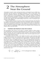
FIGURE 3.1 An acoustic pressure wave of frequency 4 kHz and pressure amplitude 0.2 Pa
traveling from left to right with speed of sound 340 m s
–1
. The upper plot shows pressure versus
distance at time t = 0 and below that a visualization of the compressions and rarefactions in the
air along the longitudinal wave. The lower plot shows the pressure variations a quarter period or
ƫVODWHUGXULQJZKLFKWLPHWKHZDYHKDVWUDYHOHGDGLVWDQFH
cT // .4 4 21 25L cm
.
3588_C003.indd 29 11/20/07 4:37:29 PM
© 2008 by Taylor & Francis Group, LLC
30 Atmospheric Acoustic Remote Sensing
Because of the wide dynamic response of the human ear, it is common to use a logarith-
mic scale for sound intensity. The sound pressure level measured in dB (decibels) is
L
p
p
p
¤
¦
¥
¥
¥
¥
´
¶
µ
µ
µ
µ
10
10
2
0
2
log ,
rms
(3.9)
where the reference pressure p
0
= 20 µPa is the very small rms pressure uctuation
which is at the threshold of hearing. Note that sound intensity is proportional to the
square of the pressure amplitude, which is why pressures are squared in (3.9). At
the other extreme of intensity is the threshold of pain, for which L
p
=120dB (or
p
rms
= 20 Pa). In practice, the human ear has some frequency sensitivity and a modi-
ed scale can be used with “a weighted response” and measured in dBA to allow for
this. But in the case of SODAR, RASS, and tomography, the interest is generally in
the response of transducers and so L
p
is used, or alternatively a logarithmic intensity
level
L
I
I
I
¤
¦
¥
¥
¥
´
¶
µ
µ
µ
µ
10
10
0
log
(3.10)
also measured in dB, where I is the sound intensity in W m
–2
and the reference inten-
sity corresponding to the threshold of hearing is I
0
=10
−12
Wm
–2
. For example, if a
SODAR is transmitting 1 W of acoustic power, then at 1 m from the source, the 1 W
is spread over an area of 4π m
2
giving an average intensity round the entire SODAR of
1/4πWm
–2
. The intensity level would be
L
I
10 1 4 10 109
10
12
log (( / ) / )P
dB.
This is only meaningful if the sound is omnidirectional: in practice, SODAR trans-
ducers and antennas are designed to be very directional, and so the intensity level
could be much higher directly in the acoustic beam. Also it is important to note that
acoustic power is referred to, since the total electrical power delivered to a speaker
is generally much higher than the transmitted acoustic power.
3.2 FREQUENCY SPECTRA
Background acoustic noise, the received echo signals, and even the transmitted signal
are not composed of single-frequency sinusoidal waves. It is therefore useful to record
and plot frequency spectra which show how much acoustic power there is per unit
frequency interval. Since the phase of the received sound is usually not of interest (an
exception is acoustic travel-time tomography), power spectra are usually recorded.
Suppose that an acoustic pressure pft
00
2cos( )P is recorded in a narrow fre-
quency band ∆f centered on frequency f
0
, together with other values at other frequen-
cies. If we multiply the entire input signal by cos( )2
0
Pft and integrate over a long
time then the result for the band around f
0
is
pt
0
2$ /
. For any other frequency f
1
,
the gradual phase shift between cos( )2
0
Pft and cos( )2
1
Pft means that their product
averages to zero. In this way, each individual spectral density component can be
recovered from any general signal. The method is generalized using complex expo-
nential notation, and taking
3588_C003.indd 30 11/20/07 4:37:38 PM
© 2008 by Taylor & Francis Group, LLC
Sound in the Atmosphere 31
Pf pt t
ft
() () ,
c
c
°
ed
-j 2P
(3.11)
which is known as the Fourier transform of a signal p(t), and the inverse Fourier
transform is
pt P f f
ft
() ( ) .
c
c
°
ed
j2P
(3.12)
In practice, signals are invariably sampled at discrete times m∆t (m = 0, 1, 2, …,
M −1), so
Pf p t p t
m
fm t
m
fm t
m
M
()y
c
c
°
£
ed e
jj22
0
1
PP$$
$
For symmetry in the inverse transform, the power spectrum is also estimated at
discrete frequencies m∆f (m = 0, 1, 2, …, M − 1), so (omitting the ∆t)
Pp n M
nm
mn f t
m
M
z
£
e
j2
0
1
01 1
P$$
,,,,.
(3.13)
Within the total sampling time of M∆t, the lowest frequency having a complete
cycle is ∆f =1/(M∆t). The highest frequency in the power spectrum is therefore
M∆f =1/∆t. However, at each frequency interval the signal has both an amplitude
and a phase (with respect to t = 0), so spectral densities at frequencies from 1/(2∆t)
to 1/∆t are really just further information about the signal components in frequency
intervals from 0 to 1/(2∆t). For this reason, the highest frequency recorded, called
the Nyquist frequency, is f
N
=1/(2∆t). The sampling frequency is f
s
=2f
N
, or in other
words the signal is sampled at twice the highest frequency for which a spectral esti-
mate is obtained.
What if the original signal contained components at higher frequencies than f
N
?
These are frequencies for which n=M+q in (3.13) where q lies between −M/2 and
M/2. From (3.13)
3588_C003.indd 31 11/20/07 4:37:42 PM
© 2008 by Taylor & Francis Group, LLC
32 Atmospheric Acoustic Remote Sensing
Pp
p
nm
mn M
m
M
m
mM q M
m
M
£
e
e
j
j
2
0
1
2
0
1
P
P
/
()/
££
£
p
p
m
mq M m
m
M
m
mq M
ee
e
jj
j
22
0
1
2
PP
P
/
/
(cos 222
0
1
2
0
1
PP
P
mm
p
P
m
M
m
mq M
m
M
q
-j
e
sin )
.
/
£
£
j
This means that any signal components having frequencies above f
N
appear at lower
frequency positions within the spectrum. This is called aliasing. Aliased compo-
nents add to the components which are really at a lower frequency, and this can cause
a very distorted impression of the true spectrum. For this reason, low-pass anti-alias-
ing lters should be used to remove all signal components above the Nyquist fre-
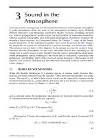
quency, prior to digitizing the signal. An example of aliasing is given in Figure 3.2
where f
N
= 2000 Hz. Note that when a signal component is at f
N
+ 500 Hz, it adds to
any other components at f
N
– 500 Hz. In this MATLAB®-generated plot, the spec-
tral density scaling for the FFT routine is N/2.
There is a very efcient method, called the fast Fourier transform (FFT), for
doing the sums required to perform the Fourier transform.
3.3 BACKGROUND AND SYSTEM NOISE
An acoustic remote-sensing system must detect signals in the presence of back-
ground and system noise. Random noise sources include electronic noise from the
instrument’s circuits, and acoustic noise from the environment. In addition, unwanted
reections from nearby buildings or trees (“xed echoes”) can obscure a valid sig-
nal, but these are not random noise.
Electronic noise comes from the noise in the preamplier, from resistors near
the front end of the instrument’s amplier chain, and from microphone self-noise.
It is most important that these noise sources are minimized, since noise voltages
from this point receive the greatest amplication. A good operational amplier can
have typically 1 nV Hz
−1/2
referred to its input. This means that if the bandwidth is
100 Hz, then the equivalent rms noise voltage at the input of the operational ampli-
er is 10 nV. Input resistors, and the resistance in the speaker/microphone, also con-
3588_C003.indd 32 11/20/07 4:37:43 PM
© 2008 by Taylor & Francis Group, LLC
Sound in the Atmosphere 33
tribute noise of about 0.1 nV Hz
–1/2
8
–1/2
. This means that the resistor noise can be
comparable to op-amp noise if the input resistors are 100
8.
A readily obtainable low-noise microphone, such as the Knowles MR8540, has a
self-noise SPL of 30 dB for a 1 kHz bandwidth, or an equivalent input
RMS acoustic
pressure of 6 × 10
–4
Pa. Given a sensitivity of -62 dB relative to 1 V/0.1 Pa, its noise
output is (10
–62/20
/0.1) (6×10
–4
)/(1000
1/2
)=160nVrms/Hz
–1/2
. Hence microphone
self-noise can be expected to be a dominant system noise source.
Background acoustic noise can vary hugely with site, with airports and roadsides
being particularly noisy. Acoustic remote-sensing systems generally use very nar-
row band-pass lters (perhaps 100 Hz wide), so most pure tones, such as from birds,
are excluded, and much of the broadband acoustic noise is also greatly reduced. It
is important, if the dynamic range of the instrumentation is limited, to band-pass
lter at an early stage in the amplier chain, so as to remove such noise components
before they saturate the circuits and cause distortion. Figure 3.3 shows some mea
-
sured background noise levels.
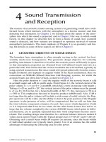
These and similar measurements by others suggest a simple power-law depen-
dence on frequency of the form
NN
f
f
q
¤
¦
¥
¥
¥
´
¶
µ
µ
µ
µ
0
0
,
(3.14)
FIGURE 3.2 Cosine signals sampled at f
s
= 4000 Hz with M = 512 samples. Upper plot: the
signal is the sum of a cosine at 1500 Hz and a cosine at 1750 Hz. Lower plot: the signal is the
sum of a cosine at 1500 Hz and a cosine at 2500 Hz.
3588_C003.indd 33 11/20/07 4:37:46 PM
© 2008 by Taylor & Francis Group, LLC
300
200
100
0
0 200 400 600 800 1000 1200 1400 1600 1800 2000
Spectral Density
600
400
200
0
Spectral Density
Frequency (Hz)
0 200 400 600 800 1000 1200 1400 1600 1800 2000
Frequency (Hz)
34 Atmospheric Acoustic Remote Sensing
where N is the noise intensity per unit frequency interval (W m
–2
Hz
–1
) and f is the
frequency. Based on the above measurements, extended to 20 kHz,
q ~ 2.8, 1.4, and
0.5 for daytime city, daytime country, and nighttime country readings, respectively.
3.4 REFLECTION AND REFRACTION
When a sound wave meets an interface where the sound speed changes, some energy
is reected and some continues across the interface but with a change in direction.
This can be visualized using the Huygens principle, which states that each point on
a wavefront acts like a point source of spherical wavelets, and taking the tangential
curve to the wavelets after a short time gives the position of the propagated wavefront.
Imagine a plane wavefront meeting a horizontal interface between medium 1 and
medium 2 at an angle of incidence R
i
as shown in Figure 3.4. From the construction
in medium 1, it can be seen that the triangles ABC and CDA are identical and that
the angle of incidence is equal to the angle of reection.
ri
.
(3.15)
Also
AC
BC AE
sin sinQQ
it
or
cc
21
sin sin
,
ti
(3.16)
which is Snell’s law.
Generally, for sound traveling through the air, there is no distinct interface but
rather a continuous change in sound speed due to a temperature gradient or wind
0 2000 4000 6000
–40
–20
0
–60
Frequency (Hz)
dB (arbitrary zero)
City day
Country day
Country night
FIGURE 3.3 Power spectra of background acoustic noise at typical sites, given in dB.
3588_C003.indd 34 11/20/07 4:37:50 PM
© 2008 by Taylor & Francis Group, LLC
Sound in the Atmosphere 35
shear. In the case where the atmosphere is horizontally uniform and the vertical
sound speed gradient dc/dz is constant,
cc
cc
c
z
z
0
0
2
0
11
sin sin
cot
Q
¤
¦
¥
¥
¥
´
¶
µ
µ
µ
µ
d
d
¤
¦
¥
¥
¥
´
¶
µ
µ
µ
µ
d
d
z
x
2
or, upon integrating,
()(),
(/)tan
,xx zz r x
c
cz
z
c
0
2
0
22
0
0
0
0
0
dd Q
ddd ddcz
r
c
cz/
,
(/)sin
.
0
0
Q
(3.17)
The sound propagation path is therefore along a circular arc of radius r and center
(x
0
, z
0
). However, the curvature is usually very small. For example, if c
0
=340ms
–1
and R
0
= π/10, the radius of curvature for an adiabatic lapse rate is 67000 km. So in
most situations involving acoustic remote-sensing, refraction can be ignored.
The fraction of incident energy reected from the atmosphere is extremely small
(see later) but for most other surfaces and for the frequency ranges typically used for
acoustic remote sensing, virtually all sound is reected. This is an important con-
sideration for siting of acoustic remote-sensing instruments, since even reections
from very distant solid objects can masquerade as genuine atmospheric reections
(known as “clutter” or “xed echoes”).
t
!
t
!
tt
c
c
t
c
t
#
t
#
i
#
r
"!
t
"!
t
FIGURE 3.4 A wavefront AB incident at an angle R
i
at time t = 0 and meeting an interface
between medium 1 and medium 2 at point A. After a time ∆t the ray from point B meets the
interface at C and the Huygens wavelet for the backward, reected, wave has reached point
D. The line CD denes the reected wavefront. The Huygens wavelet in medium 2 is shown
traveling at speed c2>c1, and the transmitted, or refracted, ray reaches point E in time ∆t.
The line CE denes the refracted wavefront.
3588_C003.indd 35 11/20/07 4:37:53 PM
© 2008 by Taylor & Francis Group, LLC
36 Atmospheric Acoustic Remote Sensing
In the case of acoustic travel-time tomography where the propagation path is at
a few meters above the ground, ground reections can be a major consideration. In
this case, the reection from the ground can combine out of phase with the direct
line-of-sight signal, causing a much reduced signal amplitude. For this reason, as
discussed further later, continuous encoded-signal systems may experience difcul-
ties and short pulses are generally used.
3.5 DIFFRACTION
SODARs and RASS use antennas, which make the source and the receiver extend
over a larger area. The acoustic pressure at some point R is the sum of all the pres-
sure contributions from small areas S dZ dS on the antenna surface, as shown in
Figure 3.5. The pressure contribution at R from an element at position S will be
proportional to the element’s area, giving
dedd
j
p
A
R
tkR
()
()
()
R
RY R
W
allowing for spherical spreading, the phase at R compared with the phase at r, and an
amplitude A varying with position on the antenna.
Also, R = r − S so for distances R>>S,
RRRr r r y
22
2 RR R Q YFsin cos( )
and, if the antenna gain is uniform across the antenna,
p
A
r
tkr
k
§
°
2
1
0
P
P
YF
W
RQ YF
P
e
ed
j
j
()
sin cos( )
()
©©
¨
¨
¨
·
¹
¸
¸
¸
°
RRd
0
a
,
x
y
z
r
R
FIGURE 3.5 The geometry of contributions to the pressure at R from points on the surface
of an antenna.
3588_C003.indd 36 11/20/07 4:37:57 PM
© 2008 by Taylor & Francis Group, LLC
Sound in the Atmosphere 37
where a is the antenna radius. The integral in the square brackets is the Bessel func-
tion J
0
(kS sin R) and
Jxxx xJx
x
01
0
() (),d
°
so
p
A
r
a
Jka
ka
tkr
§
©
¨
¨
·
¹
¸
¸
e
j( )
()
(sin)
sin
W
P
Q
Q
2
1
2
(3.18)
The oscillatory nature of the last term in square brackets is known as a diffrac-
tion pattern. It arises because the antenna is not producing a plane wave, but has
nite width. This pattern is shown in Figure 3.6. Bands of energy occur at periodic
values of R, which are known as side lobes. Depending on the ratio of radius a to
wavelength M, these side lobes can send acoustic power out at low angles and cause
reception of echoes from buildings or other structures nearby. It can be seen that the
rst zero crossing is at ka sin R = 3.83, so, for example, if a dish of radius 1 m is used
at a wavelength of 0.1 m, then the rst zero occurs at
R =sin
–1
(3.83/62.83) = 3.5° and
the resulting beam is 7° in width.
Similar oscillating diffraction patterns occur whenever sound impinges on an edge.
3.6 DOPPLER SHIFT
Doppler shift is a change in the frequency of a signal caused by a moving source or
target. Imagine a target (a patch of turbulence, for example) moving in the direction
of propagation at a speed u and the speed of sound is c, as in Figure 3.7.
ka
J
ka ka
FIGURE 3.6 The diffraction pattern from a circular aperture of uniform gain.
3588_C003.indd 37 11/20/07 4:38:00 PM
© 2008 by Taylor & Francis Group, LLC
38 Atmospheric Acoustic Remote Sensing
At time t = 0, an acoustic pressure maximum is at the target, and the next pres-
sure maximum is a distance M away. If this next pressure maximum reaches the
target at t = T
D
, the target has moved a distance uT
D
and the pressure maximum has
moved a distance cT
D
= M+ uT
D
. So the period between two maxima at the target is
T
D
= M/(c−u). The frequency of the sound at the target is therefore
f
T
cu c u
c
f
u
c
D
D
¤
¦
¥
¥
¥
¥
´
¶
µ
µ
µ
µ
¤
¦
¥
¥
¥
¥
´
1
11
LL
¶¶
µ
µ
µ
µ
. (3.19)
The Doppler frequency f
D
is less than the transmitted frequency, as sensed by
the target.
If the sound is reected by the target back toward the source, successive pressure
maxima are separated by a larger distance, as shown in Figure 3.8.
Now
LL
DD
() ,cuT
cu
cu
so
ff
cu
cu
f
u
c
D
y
¤
¦
¥
¥
¥
´
¶
µ
µ
µ
12 .
(3.20)
The change in frequency is approximately 2(u/c)f. This frequency change is used
to determine the wind speed components carrying turbulent patches. More compli-
cated geometries will be considered in Chapter 4.
In the acoustic travel-time tomography situation, both the source and the receiver
are stationary, and separated by a distance x = X. If the air is moving at speed u(x)
along the line from the source to the receiver, then the time taken for a pressure
maximum to move from the source to the receiver is
t
x
cx ux
X
downwind
d
°
() ()
0
(3.21)
uT
D
cT
D
u
λ
c
FIGURE 3.7 A turbulent patch moving with speed u in the direction of sound propagation.
The lower plot shows the distance moved by the patch in time T
D
, and the distance moved by
the acoustic pressure wave in the same time.
3588_C003.indd 38 11/20/07 4:38:06 PM
© 2008 by Taylor & Francis Group, LLC
Sound in the Atmosphere 39
and in the opposite direction
t
x
cx ux
X
upwind
d
°
() ()
,
0
(3.22)
where both wind speed and sound speed can, in general, vary along the path. These
times are identical for successive pressure maxima so there is no Doppler shift.
However, the downwind and upwind travel times can distinguish temperature varia-
tions (changes in c) from wind speed variations (changes in u) since u<<c and
tt
x
cuc
dx
cuc
X
upwind downwind
d
°
(/) (/)11
00
XXX
u
c
x
c
u
c
x
c
°°
y
¤
¦
¥
¥
¥
´
¶
µ
µ
µ
¤
¦
¥
¥
¥
´
¶
µ
µ
µ
1
1
0
0
d
d
XXX X
ux
c
tt
x
c
°° °
yy22
2
00
d
d
upwind downwind
,.
(3.23)
3.7 SCATTERING
Scattering of sound by turbulence has been very thoroughly investigated theoreti-
cally (Tatarskii, 1961; Ostashev, 1997). Here we give a more intuitive description,
together with some new results relating to SODARs.
3.7.1 SCATTERING FROM TURBULENCE
Scattering occurs when an object with a sound speed different from air causes rays
from the wavefront to deviate into many directions. In the case of scattering from
turbulent temperature uctuations, there are many randomly placed and randomly
sized scatterers, each having a density very slightly different from the average air
density. Scattering can also be caused by the random motion of the turbulent patches
uT
D
cT
D
u
λ
c
c
cT
D
λ
D
FIGURE 3.8 Reection of sound from a target moving in the direction of sound propaga-
tion. The dashed lines show positions of reected pressure maxima at a time T
D
after the rst
pressure maximum reaches the target patch.
3588_C003.indd 39 11/20/07 4:38:09 PM
© 2008 by Taylor & Francis Group, LLC
40 Atmospheric Acoustic Remote Sensing
since this too causes a change in the local sound speed. The strength of such scatter-
ing (how much energy is deected) depends on the magnitude of the variations
`
c
in sound speed. From (3.2) for temperature uctuations T'
`
`
y
c
T
c
T
c
T
d
d
1
2
. (3.24)
Generally sound speed variations are expressed as refractive index uctuations
of magnitude
`
`
n
c
c
. (3.25)
For a uctuation V' in the vector wind, the sound speed uctuation depends on
the direction of V' compared to the direction of propagation
ˆ
k of the sound (
ˆ
k is a
unit vector). The combination of temperature and velocity uctuations gives refrac-
tive index uctuations
`
`
`
n
Vk
c
T
T
ˆ
.
2
(3.26)
The following chiey relates to SODARs since they obtain a signal through
reections from turbulence. The SODAR beam and pulse duration U dene a volume
that contains refractive index uctuations
`
n continuously varying in strength and
spatial scale. Scattering from this volume is a three-dimensional problem, but the
general ideas can be more easily understood by considering propagation and scat-
tering of sound in just the vertical, z, direction. Consider two layers spaced by l and
having refractive index uctuations
`
nz() and
`
nz l() as shown in Figure 3.9.
The amplitude from a single uctuation is proportional to
`
n . The sound inten-
sity I is proportional to the square of the sum of all the individual scattered ampli-
tudes and contains terms like
Inznzl
kl
s
``
() ( ) .e
j 2
(3.27)
The bar over the refractive index prod-
uct means that the uctuations have been
averaged over time, and the exponential
term accounts for the path difference of
2l for backscatter from the patches at z
and at z+l (i.e., this is a phase term). The
wavelength of the transmitted sound is
M and the corresponding wavenumber
is k =2π/M. Integrations must be per-
formed over the z range ±cU/2 of the
SODAR scattering volume, and over the
separations l, thus
z
l
n´(z)
n´(z + l)
FIGURE 3.9 The geometry of two scat-
tering layers.
3588_C003.indd 40 11/20/07 4:38:20 PM
© 2008 by Taylor & Francis Group, LLC
Sound in the Atmosphere 41
I n z n z l dz l
z
kl
l
s
``
Đ
â
ă
ă
ã
ạ
á
á
() ( ) .ed
j 2
(3.28)
The term in square brackets is called the spatial autocorrelation function of uctua-
tions
`
n . This decreases with increasing separation l between turbulent layers as they
become increasing uncorrelated and
`
nz() and
`
nz l() are less likely to increase
or decrease together. The autocorrelation of refractive index uctuations therefore
contains information about spatial scales of turbulence. This information could also
be expressed in terms of spatial frequencies by taking the Fourier transform of this
autocorrelation function. The WienerKhinchine theorem shows that the Fourier
transform of the autocorrelation function is the power spectrum, '
n
, of
`
n
, or
&
n
z
l
l
nznz l z l() ()( ) .K
K
``
Đ
â
ă
ă
ã
ạ
á
á
de d
j
(3.29)
Using the inverse Fourier transform, Eq. (3.28) can be written in the form
Il
n
kl k l
l
| & () ,KK
K
ede d
jj
Đ
â
ă
ă
ã
ạ
á
á
2
(3.30)
where L is a spatial wavenumber, KP 2/d , for refractive index uctuations of size
d as in (2.13) of Chapter 2. This can be rearranged
Il
n
kl
c
c
| & ()
()
/
/
KK
K
T
T
K
edd
j
Đ
â
ă
ă
ă
ã
ạ
á
á
á
2
2
2
(3.31)
The term in square brackets is the Fourier transform of a rectangular function of
length cU
el
ckc
kl
c
c
j
d
()
/
/
sin[( ) / ]
(
2
2
2
2
22
2
K
T
T
TKT
kkcK T)/
,
2
(3.32)
which has the shape shown in Figure 3.10.
The zero crossings occur at
2
4
k
c
oK
P
T
. (3.33)
Typical values for a SODAR are cU = 8.5 m, or 4/cU =0.7m
1
, and M = 0.08 m, or
k =80m
1
. So L is very nearly equal to 2k, and the term in square brackets in Eq.
(3.32) is like a delta-function DK P T(/)o24kc, which has the property
&&
nn
k
c
k
c
()KDK
P
T
K
P
T
K
o
Ô
Ư
Ơ
Ơ
Ơ
Ơ
ả
à
à
à
à
o
Ô
Ư
2
4
2
4
d
ƠƠ
Ơ
Ơ
Ơ
ả
à
à
à
à
. (3.34)
3588_C003.indd 41 11/20/07 4:38:34 PM
â 2008 by Taylor & Francis Group, LLC
42 Atmospheric Acoustic Remote Sensing
The result is that
Ik
c
n
| & 2
4
o
¤
¦
¥
¥
¥
¥
´
¶
µ
µ
µ
µ
P
T
. (3.35)
This means that the reected sound intensity depends on the strength of refrac-
tive index uctuations having spatial wavenumbers of twice the wavenumber of the
transmitted sound. This can be interpreted simply as follows. The scattered sound
is very weak, but scatterings separated vertically by d = M/2 will add in phase (there
is no π phase change on reection for soft scattering). This means that L= 2π/d =
2π/(M/2) = 2k as predicted by (3.35).
The above simplied analysis applies for scattering directly back to a “monos-
tatic” SODAR which has speakers and microphones located at the same place. The
situation is more complicated for “bistatic” SODARs for which the scattering angle
is not 180°. Figure 3.11 shows scattering through an angle
C from two turbulent
patches at positions A and B which are in layers separated by l. As in the case of
180° scattering, the incident ray (shown as a dark line) is at an angle C/2 to the layers.
The extra path length for sound scattered from B, compared to that scattered from
A, is distance ABC where
ABC
ll
12
2
2
2
sin( / )
sin( / )
sin .
BP
B
B
(3.36)
When the path difference ABC equals M, a strong signal results because the scat-
tered waves are then in phase.
The intensity in the general case is therefore proportional to
&
n
kc(sin(/) /)224BPTo where cU is a typical dimension of the scattering volume.
For example, if the frequency is 5100 Hz, then for backscatter 2
k ~ 2π 60 m
–1
and the
volume correction term 4π/cU is small providing cU >> 1/60 m. The theory predicts
very tight dependence on the Bragg wavenumber 2ksin(C. Also, it is often con-
kc
k ckc
FIGURE 3.10 The Fourier transform of a rectangular function of length cƲ
3588_C003.indd 42 11/20/07 4:38:38 PM
© 2008 by Taylor & Francis Group, LLC
Sound in the Atmosphere 43
venient to think of the turbulent wavenumber as being a measure of turbulent eddy
size, since eddies spaced by L can be thought of as having dimensions of approxi-
mately 2π/L. This means that a SODAR of wavelength M set up so that scattering
is through an angle C, will record echo information about the intensity of refractive
index uctuations of size
d
c
o
L
BLT22sin( / ) /
. (3.37)
As an example, if the wavelength is 0.1 m (typical of a SODAR operating at
3.4 kHz) and the pulse duration is 50 ms, then cU = 10 m and for monostatic sound-
ing (with C = 180°), d = 0.0498 to 0.0503 m.
It should not be thought from the above that all the turbulent patches of size d
somehow “line up” to give a resonant back-scatter in the manner of regular Bragg
scattering from a crystal. Rather, the incident wavetrain picks out those spatial Fou-
rier components which give the strongest combined reection. Physically, we can
imagine a spatial arrangement of uctuations multiplied by a sine wave. Averaging
over the record length then gives a measure of the combined strength of reections.
But this process is identical to nding the coefcients in a Fourier series, which can
be generalized via Fourier transforms.
3.7.2 INTENSITY IN TERMS OF STRUCTURE FUNCTION PARAMETERS
From the previous section it is clear that the scattered acoustic intensity received
by a SODAR is proportional to the power spectrum, &
n
k(sin(/))22B , of refrac-
tive index uctuations at spatial wavenumbers close to &
n
k 2
2
sin( /B . What is
the connection between '
n
and the turbulence parameters such as C
V
2
and C
T
2
l
l
l
FIGURE 3.11 The geometry of scattering for the general bi-static SODAR case, where
VFDWWHULQJLVWKURXJKDQJOHơIURPOD\HUVVHSDUDWHGE\GLVWDQFH l.
3588_C003.indd 43 11/20/07 4:38:46 PM
© 2008 by Taylor & Francis Group, LLC
44 Atmospheric Acoustic Remote Sensing
discussed in Chapter 2? Since '
n
arises from the Fourier transform of terms like
``
nznz l() ( ) in (3.29) and from (3.26)
`
`
`
nVkcT T
//2
, we would expect
'
n
to be the sum of terms containing the power spectra of the autocorrelation func-
tions of [()
][ ( )
]
`
`
VzkVz lk and
``
TzTz l() ( ). In general, there would also be
cross-terms in
``
VT but it is usually assumed that the uctuations in velocity and
temperature are uncorrelated and so the cross-terms vanish. Writing, as in (3.29),
&
V
z
Vz kVz l k z() [ ()
][ ( )
]K
`
`
Đ
â
ă
ă
ã
ạ
á
á
de
jKK
K
K
l
l
T
z
l
l
TzTz l z
d
de
j
,
() () ( )
``
Đ
â
ă
ă
ã
ạ
á
á
& ddl
l
,
(3.38)
then from (3.26)
&
&
n
T
k
k
T
2
2
22
4
2
sin cos
(sin(/))
B
B
B
Ô
Ư
Ơ
Ơ
Ơ
Ơ
ả
à
à
à
à
22
2
2
1
42
22
Ô
Ư
Ơ
Ơ
Ơ
Ơ
ả
à
à
à
à
Đ
â
ă
P
B
B
cos
(sin(/))&
V
k
c
ăă
ă
ã
ạ
á
á
á
. (3.39)
The dot product in
`
Vzk()
gives a cosine of the angle between
`
Vz()
and
k .
Averaging over the square of such terms for a total scattering angle of C gives the
( / )cos ( / )14 2
2
PB
term. The cos
2
B term allows for the fact that the reections
from the two turbulent patches at A and B in Figure 3.11 are not diffuse.
From Chapter 2, &
VV
C() .
/
KK
076
253
and &
TT
C
0 033
253
.
/
K , so the intensity from
combined temperature and velocity uctuations is
I
C
T
C
TV
| cos . . cos
2
2
2
2
2
0033 076
2
B
B
Ô
Ư
Ơ
Ơ
Ơ
Ơ
ả
à
à
à
à
PPc
2
Đ
â
ă
ă
ă
ã
ạ
á
á
á
. (3.40)
This has the very interesting property that acoustic backscatter (with C =180)
from turbulence depends only on the temperature uctuations. Monostatic SODARs
are therefore insensitive to mechanical turbulence and give very low signals in near-
neutral conditions when there is little temperature contrast.
3.7.3 SCATTERING FROM RAIN
Rain can be a signicant source of acoustic echoes for SODARs. Each drop acts
as an individual scatterer and, since a drop diameter D is small compared with the
wavelength M, Rayleigh acoustic scattering is a good approximation. In this approxi-
mation, the entire drop volume experiences the same acoustic pressure at any one
time, and all parts of the drop radiate acoustic energy in phase, so the scattered
amplitude is proportional to the drop volume, or to diameter D cubed. The scattered
intensity I
s
is proportional to the incident intensity I
i
, to the square of the scattered
amplitude, and also decreases with distance r squared (i.e., spherical spreading).
Assume that there is also a dependence on wavelength M to the power q, so
3588_C003.indd 44 11/20/07 4:39:00 PM
â 2008 by Taylor & Francis Group, LLC
Sound in the Atmosphere 45
I
I
A
D
r
q
s
i
6
2
L ,
where A is a dimensionless constant. Since the left side is dimensionless, q =−4.
When a full solution of the acoustic wave equation is done, each drop acts as if there
is an equivalent plane area scattering all incident energy. This equivalent cross-sec-
tion area, per unit solid angle into which the sound is scattered, is called the differ-
ential scattering cross-section T
R
, and is given by
S
P
B
L
R
5
2
6
4
36
23(cos).
D
(3.41)
Figure 3.12 shows the angular dependence of this rain scattering, together with the
angular dependence of scattering by turbulent temperature and velocity uctuations.
The relative acoustic intensities from the three scattering mechanisms at any angle
depend on the magnitudes of rainfall intensity R, C
T
2
, and C
V
2
, and since generally
C
V
2
>> C
T
2
the scattered intensity from velocity uctuations can exceed those from
temperature uctuations within a few degrees of the back-scatter direction.
It is worth noting that the peak scattered intensity from turbulence for bi-static
SODARs occurs at an angle C given by
90
60
30
330
300
270
240
210
180
150
120
1
0.8
0.6
0.4
0.2
0
FIGURE 3.12 The angular dependence of scattering in the backward direction: from rain
VROLGOLQHIURPWHPSHUDWXUHÁXFWXDWLRQVGRWWHGOLQHDQGIURPYHORFLW\ÁXFWXDWLRQVGDVKHG
line). Arbitrary scaling has been used.
3588_C003.indd 45 11/20/07 4:39:07 PM
© 2008 by Taylor & Francis Group, LLC
46 Atmospheric Acoustic Remote Sensing
d
dB
B
B
cos cos
22
2
0
¤
¦
¥
¥
¥
¥
´
¶
µ
µ
µ
µ
or cos C= −2/3, which is exactly where the scattering from rain has a minimum. Bi-
static SODARs are therefore less susceptible to rain clutter.
The total differential acoustic scattering cross-section for rain includes scatter-
ing from drops of all diameters, weighted according to the numbers n
D
(D)dD of
drops per unit volume having diameters between D and dD. A commonly assumed
probability distribution for raindrop diameters is the Marshall–Palmer distribution
(Marshall and Palmer, 1948)
nD n
D
D
() ,
0
e
,
(3.42)
where n
0
=8×10
6
m
–4
for drop diameters D in m and ,
4100
021
R
.
m
–1
for rain-
fall intensity R in mm h
–1
. Integrated over all drop sizes (in practice limited to about
6 mm maximum diameter), there are about 2000 drops per m
3
for R =1mmh
–1
. The
integrated differential scattering cross-section is
SP B
L
R
20 2 3
52
0
47
(cos)
n
,
(3.43)
or typically 10
–11
m
2
per m
2
. Comparison of this cross-section with that from tur-
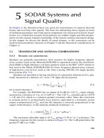
bulence will be discussed in Chapter 4. Figure 3.13 shows power spectra measured
using an AV4000 SODAR operating at 4500 Hz.
0
100
200
300
400
500
600
0 102030405060
Spectral Bin
Power Spectral Density
FIGURE 3.13 Power spectra recorded from a vertically pointing SODAR with: no rain
(dotted curve), 5 to 10 mm/h (thin line), and greater than 10 mm/h rain (heavy line).
3588_C003.indd 46 11/20/07 4:39:12 PM
© 2008 by Taylor & Francis Group, LLC
Sound in the Atmosphere 47
3.8 ATTENUATION
3.8.1 LOSSES DUE TO SPHERICAL SPREADING
Equation (3.4) describes a plane wave in which there is no variation in intensity in
the x and y directions. In practice, the sound spreads out from a localized source such
as a SODAR. If the transmitted power, P
T
, is spread out evenly into a sphere of radius
r, then the intensity at distance r from the source would be
I
P
r
power
area
T
4
2
P
. (3.44)
The intensity clearly decreases with range squared. From (3.9), this is equivalent
to a loss of 20 log
10
2=6dB for every doubling of range. This is one reason for the
limited range of SODAR and RASS instruments.
3.8.2 LOSSES DUE TO ABSORPTION
When sound travels a small distance through air, the intensity I decreases a small
amount ∆I due to absorption losses. The amount of intensity decrease depends on the
distance ∆x traveled and also depends on the initial energy, so $$IIx| , or
d
d
I
I
xA , (3.45)
where B is the absorption coefcient. If B does not vary along the sound path, then
integrating gives
II
x
0
e
A
. (3.46)
The absorption coefcient B is the sum of classical absorption, B
c
, and molecular
absorption, B
m
. Classical absorption is due to each small volume of air being com-
pressed and stretched by the sound pressure along the direction of propagation, and
so causing a shape change or shear, which is resisted by viscous forces. The energy
loss per cycle is proportional to the shear, which is proportional to the size of the
volume affected or to the wavelength M. The energy loss per second is therefore pro-
portional to the square of frequency, f
2
. This means that energy loss per unit length
is also proportional to f
2
.
Molecular absorption is due to transfer of a molecule’s energy out of the transla-
tional motion and into vibration or rotation of the molecule. For dry air consisting of
N
2
and O
2
molecules, any extra energy transferred to rotation during a sound pressure
impulse is transferred back into translational energy in a very short time compared
to the sound wave period. For these molecules, the “relaxation time” for rotational
modes is very short. On the other hand, excess energy is not transferred efciently to
vibrational modes because their relaxation time is very long. So dry air does not have
much molecular absorption. However, when water vapor molecules are present, the
transfer of energy to vibrational modes in N
2
and O
2
occurs in a very much shorter
time through collisions with H
2
O. But at high humidities, O
2
and N
2
molecules are
3588_C003.indd 47 11/20/07 4:39:18 PM
© 2008 by Taylor & Francis Group, LLC
48 Atmospheric Acoustic Remote Sensing
fully excited in their vibration mode without acoustically enhanced collisions, and
there is again little extra energy taken out of the pressure wave. Absorption also
depends on temperature and pressure since these affect collisions. Absorption in
dB m
1
is a very complicated formula (Salomons, 2001)
A
M
r
8 686
184 10
0 1068 3352
2
11
0
.
.
.exp(/
2
fp
p
f
N
TT
ff
fT
ff
). exp( ./)
NN
2
2
2
22 22
0 01275 2239 1
Đ
O
ââ
ă
ă
ă
ã
ạ
á
á
á
ê
ô
ơ
ằ
ẳ
M
3
0
2
928
,
[f
p
p
N
00
24 40400
002
03
417 1
0
3
2
q
f
p
p
q
q
e
O
.( )
],
.
.
M
M
991
10 62
0
Ô
Ư
Ơ
Ơ
Ơ
Ơ
ả
à
à
à
à
Ô
Ư
Ơ
Ơ
Ơ
Ơ
ả
à
à
à
à
q
p
p
q
r
,
ln .
667 15 7372
0
1 261
1
Ô
Ư
Ơ
Ơ
Ơ
Ơ
ả
à
à
à
à
.,
,
.
T
T
T
T
M
(3.47)
where f is the frequency in Hz, T the temperature in K, p the pressure in kPa, r the
relative humidity in %, and the constants are p
0
=101.325kPa, T
0
=273.16K, and
T
1
=293.15 K. The result for several values of r is shown in Figure 3.14 at T =10C
(upper plot) and T = 20C (lower plot) and with p = 101.3 kPa. The slope is close to
that of f
2
over the usual range of SODAR frequencies from 1.5 to 6 kHz and humid-
ity ranging from 20% to 100%. A simple approximation for this range, with r in %,
f in kHz, and air temperature T
C
in the range 10 to 20C is
A
0 0018 1 10
2
0
22 0 6
1
.[ ].
/( . )
f
p
p
e
rT
C
dBm (3.48)
Absorption coefcients based on this approximation are also shown in Fig-
ure 3.14 for
f = 3 kHz. Note that absorption in dB m
1
is equal to 10 log
10
e times the
absorption in m
1
. A 2 kHz SODAR would lose an extra 40 dB due to absorption
when the humidity is 50% and temperature 10C, and 20 dB due to beam spreading
between 100 m and 1 km range. Higher frequency SODARs will have more limited
range due to absorption.
3.8.3 LOSSES DUE TO SCATTERING OUT OF THE BEAM
Similar to rain, turbulence acts as if there is an extremely small equivalent plane area
scattering all incident energy within a beam. This equivalent cross-section area, per
unit volume and per unit solid angle into which the sound is scattered, is called the
differential scattering cross-section T
s
. In Chapter 4, we will nd that
3588_C003.indd 48 11/20/07 4:39:21 PM
â 2008 by Taylor & Francis Group, LLC
Sound in the Atmosphere 49
S
B
K
B
s
Ô
Ư
Ơ
Ơ
Ơ
1
8
0033 076
2
42
11 3
2
2
2
k
C
T
T
cos
cos
/
ƠƠ
ả
à
à
à
à
Đ
â
ă
ă
ă
ã
ạ
á
á
á
C
c
k
V
2
2
13
20 3
2
2
P
B
B
/
/
cos
sin
22
0 033 0 76
2
11 3
2
2
2
Ô
Ư
Ơ
Ơ
Ơ
Ơ
ả
à
à
à
à
Ô
Ư
Ơ
Ơ
/
cos
C
T
T
B
ƠƠ
Ơ
ả
à
à
à
à
Đ
â
ă
ă
ă
ã
ạ
á
á
á
C
c
V
2
2
P
.
(3.49)
0.0001
0.001
0.01
0.1
1
10
0.1 10 100
Frequency (kHz)
Frequency (kHz)
dB/m
0.0001
0.001
0.01
0.1
1
10
dB/m
0%20 %
100%
50%
0.1 1
1
10 100
0%20 %
100%
50 %
FIGURE 3.14 Atmospheric absorption of sound in dB m
1
as a function of sound fre-
quency. Temperature T = 10C (upper plot) and T = 20C (lower plot) and with p =101.3kPa.
The individual points plotted are from Eq. (3.48).
3588_C003.indd 49 11/20/07 4:39:23 PM
â 2008 by Taylor & Francis Group, LLC
50 Atmospheric Acoustic Remote Sensing
Assume that the incident intensity is I
i
Wm
2
in a volume of cross-sec-
tion area A and small distance dz in the propagation direction. The total incident
power is I
i
A. Of this, an equivalent area A T
s
dz d scatters sound into solid angle
d=2sinC dC. Integrating over all solid angles, the equivalent scattering area is
2PSBBBd
s
zA d()sin
, giving a loss in ongoing intensity of dI I dz
iei
A where
APSBBB
es
2()sind
(3.50)
is the excess attenuation due to sound being scattered out of the beam.
Care is required to evaluate the integral in (3.50), since (3.49) suggests that
T
s
= at C = 0. However, turbulent scattering only occurs for turbulent scales up to
d = L
0
in (3.49), where L
0
is the outer scale of the inertial sub-range. The minimum
value of C for the integral in (3.50) is therefore
B
L
min
sin .
Ô
Ư
Ơ
Ơ
Ơ
Ơ
ả
à
à
à
à
2
2
1
0
L
(3.51)
The integral can be rewritten in the form
A
PM
M
e
kC
T
T
13
11 3
22
83
2
2
2
12
0033 0761
/
//
()
(22
22
2
2
2
1
0
M
P
M
L
).
/
C
c
V
L
Đ
â
ă
ă
ă
ã
ạ
á
á
á
d
The wavelength M is much smaller than L
0
, so small à terms dominate, and
A
P
P
e
y
Đ
â
ă
ă
ă
ã
ạ
á
á
kC
T
C
c
TV
13
11 3
2
2
2
2
2
0033 076
/
/
áá
y
MM
P
L
83
2
1
23 113
2
0
53
2
0
3
52
0 033
/
/
//
/
.d
L
T
kL
C
TT
C
c
V
2
2
2
076
Ô
Ư
Ơ
Ơ
Ơ
Ơ
ả
à
à
à
à
à
P
Pan-Naixian (2003) argues that scales of size L
0
do not ll the acoustic beam
for conventional SODARs, and so the appropriate limiting turbulent element size
is 2zR, where R is the beam angular half-width (typically 5). This half-width is
inversely proportional to transmitting frequency for an antenna of xed radius (as
will be seen in Chapter 4), having the form
$Q162./ka
. Also, the term in C
V
2
dominates over the term in C
T
2
, so the result is
A
e
y
Ô
Ư
Ơ
Ơ
Ơ
Ơ
ả
à
à
à
à
004
13
2
2
53
/
/
k
C
c
z
a
V
(3.52)
Pan-Naixian produces evidence for this dependence on frequency. For a transmit
frequency f
T
=3400Hz, c =340ms
1
, M =0.1m, k =63m
1
, a =0.6m, z =200m,
and C
V
2
= 0.01 m
4/3
s
2
, we nd B
e
=2ì10
4
m
1
. Further corrections for non-uni-
form intensity across the SODAR beam do not change the conclusion that B
e
<< B.
3588_C003.indd 50 11/20/07 4:39:35 PM
â 2008 by Taylor & Francis Group, LLC
Sound in the Atmosphere 51
3.9 SOUND PROPAGATION HORIZONTALLY
Acoustic travel-time tomography also relies on sound propagating through the
atmosphere, although in this case propagation is horizontal and close to the surface
(Raabe et al., 2001; Ziemann et al., 2001). Measurements are conducted using mul-
tiple paths, each of which is between an acoustic source and an acoustic receiver.
The only measurement made is the time taken for the sound to travel a path.
There is no Doppler shift since the travel time between the source and the
receiver is the same for each acoustic wavefront: if successive wavefronts are period
T apart initially, they also arrive period T apart.
The time taken to travel a xed distance r is
tr
r
cr
r
()
()
,
°
d
0
(3.53)
where 1/c is often called the slowness. The temperature and wind effects on c are
generally small, so (3.26) can be used and
11
0
1
0
0
20cr c
Vr
c
Tr T
T() ()
ˆ
()
() ()
()
y
§
©
¨
¨
·
¹
¸
¸¸
y
§
©
¨
¨
·
¹
¸
¸
1
1
0
1
0
0
20c
Vr
c
Tr T
T()
ˆ
()
() ()
()
(3.54)
giving the travel times in both directions along the path as
tr
c
r
c
Vr r
T
Tr T
r
()
() ()
(
ˆ
)
()
() (
°
1
0
1
0
1
20
0
0
d )),
()
() ()
(
ˆ
[]
§
©
¨
¨
¨
·
¹
¸
¸
¸
°
dr
tr
c
r
c
Vr
r
0
1
0
1
0
))
()
{() ()} .ddr
T
Tr T r
rr
00
1
20
0
°°
§
©
¨
¨
¨
·
¹
¸
¸
¸
(3.55)
Consequently
1
20
1
00
0[( ) ( )]
() () ()
[() ()]tr t r
r
ccT
Tr T r d ,,
[( ) ( )]
()
(
ˆ
)
0
2
0
1
2
2
0
r
r
tr t r
c
Vr r
°
°
d
(3.56)
gives separate equations for wind speed and temperature along the path. More detail
is obtained by having multiple paths and, generally, dividing the 2D sampled area
into discrete grids with each grid cell having a constant temperature and wind speed.
Each of the M paths is represented by an integral pair as in (3.56) and the measured
sums and differences of travel times can be written in the form
sTtuv
mmnn
n
N
mmnnmnn
n
N
££
GAB$
11
,( ),
(3.57)
3588_C003.indd 51 11/20/07 4:39:40 PM
© 2008 by Taylor & Francis Group, LLC