New Approaches in Automation and Robotics part 3 pdf
Bạn đang xem bản rút gọn của tài liệu. Xem và tải ngay bản đầy đủ của tài liệu tại đây (1.09 MB, 30 trang )
Neural-Based Navigation Approach for a Bi-Steerable Mobile Robot
53
Fig. 16. Robucar trajectory and evolution of steering angle and velocity (external
environment).
5. Conclusion
In the implemented neural-based navigation, the two intelligent behaviors necessary to the
navigation, are acquired by learning using GBP algorithm. They enable Robucar to be more
autonomous and intelligent in partially structured environments. Nevertheless, there are a
number of issues that need to be further investigated. At first, the Robucar must be
endowed with one or several actions to come back to eliminate a stop in a dead zone
situation. Another interesting alternative is the use of a better localization not only based on
odometry but by fusing data of other sensors such as laser scanner.
6. References
Anderson, A. (1995). An Introduction to Neural Networks. The MIT Press, ISBN: 0262011441,
Cambridge, Massachusetts, London, England.
Avina Cervantes, J.G. (2005). Navigation visuelle d'un robot mobile dans un environnement
d'extérieur semi-structuré, PhD thesis, France.
Azouaoui, O. & Chohra, A. (2003). Pattern classifiers based on soft computing and their
FPGA integration for intelligent behavior control of mobile robots, Proc. IEEE 11
th
Int. Conf. on Advanced Robotics ICAR’2003, pp. 148-154, ISBN: 972-96889-9-0,
Portugal, June 2003, Universidade de Coimbra Publisher, Coimbra.
Azouaoui, O. & Chohra, A. (2002). Soft computing based pattern classifiers for the obstacle
avoidance behavior of Intelligent Autonomous Vehicles (IAV), Applied Intelligence:
The International Journal of Artificial Intelligence, Neural Networks, and Complex
New Approaches in Automation and Robotics
54
Problem-Solving Technologies, Vol. 16, N° 3, May/June 2002, pp. 249-271, ISSN: 1573-
7497 (online).
Azouaoui, O. & Chohra, A. (1998). Evolution, behavior, and intelligence of Autonomous
Robotic Systems (ARS), Proceedings of 3rd Int. IFAC Conf. Intelligent Autonomous
Vehicles, pp. 139-145, Spain, March 1998, Miguel Angel SALICHS and Aarne
HALME editors, Madrid.
Bento, L.C. & Nunes, U. (2004). Autonomous navigation control with magnetic markers
guidance of a cybernetic car using fuzzy logic, Machine intelligence and robotic
control, Vol. 6, No.1, March 2004, pp. 1-10, ISSN: 1345-269X.
Chohra, A.; Farah A. & Benmehrez, C. (1998). Neural navigation approach for Intelligent
Autonomous Vehicles (IAV) in Partially structured Environments, International
Journal of Applied Intelligence: Artificial Intelligence, Neural Networks, and Complex
Problem-Solving Technologies, Vol. 8, No. 3, May 1998, pp. 219- 233, ISSN: 1573-7497
(online).
Gu, D. & Hu, H. (2002). Neural predictive control for a car-like mobile robot, International
Journal of Robotics and Autonomous Systems, Vol. 39, No. 2-3, May 2002, pp. 73-86,
ISSN: 0921-8890.
Hong, T.; Rasmussen, C.; Chang, T. & Shneier, M. (2002). Fusing ladar and color image
information for mobile robot feature detection and tracking, Proceedings of 7
th
International Conference on Intelligent Autonomous Systems, pp. 124-131, ISBN: 1-
58603-239-9, CA, March 2002, IOS Press, Marina del Rey.
Kujawski, C. (1995). Deciding the behaviour of an autonomous mobile road vehicle,
Proceedings of 2nd International IFAC Conference on Intelligent Autonomous Vehicles,
pp. 404-409, Finland, June 1995, Halme and K. Koskinen editors, Helsinki.
Labakhua, L. ; Nunes, U. ; Rodrigues, R. & Leite, F. S. (2006). Smooth trajectory planning for
fully automated passengers vehicles, International Conference on Informatics in
Control, Automation and Robotics, pp. 89-96, ISBN: 972-8865-60-0, Portugal,
August 2006, INSTICC Press, Setubal.
Mendes, A. ; Bento, L.C. & Nunes, U. (2003). Path-tracking controller with an anti-collision
behavior of a bi-steerable cybernetic car, 9th IEEE Int. Conference on Emerging
Technologies and Factory Automation (ETFA 2003), pp. 613-619, ISBN: 0-7803-7937-3,
Portugal, September 2003, UNINOVA-CRI and Universidade Nova de Lisboa-FCT-
DEE publisher, Lisboa.
Murphy, R. R. (2000). Fuzzy logic for fusion of tactical influences on vehicle speed control,
In: Fuzzy logic techniques for autonomous vehicle navigation, Dimiter Driankov and
Alessandro Saffiotti editors, pp 73-98, Physica-Verlag, ISBN: 978-3-7908-1341-8,
New York.
Niegel, W. (1995). Methodical structuring of knowledge used in an intelligent driving
system, Proceedings of 2nd International IFAC Conference on Intelligent Autonomous
Vehicles, pp. 398-403, Finland, June 1995, Halme and K. Koskinen editors, Helsinki.
Schafer, B.H. (2005). Detection of negative obstacles in outdoor terrain, Technical report,
Kaiserlautern university of technology, 2005.
Schilling, K. & Jungius, C. (1996). Mobile robots for planetary exploration, PControl
Engineering Practice, Vol. 4, N° 4, April 1996, pp. 513-524, ISSN: 0967-0661.
SICK. (2001). Hardware setup and measurement mode configuration, Quick manual for LMS
communication setup, SICK AG, Germany, June 2001.
Sorouchyari, E. (1989). Mobile robot navigation: a neural network approach, In Annales du
Groupe CARNAC1 no. S, pp. 13-24.
Sutton, R.S. & Barto, A. (1998). Reinforcement Learning : an Introduction. MA: MIT Press, ISBN-
10: 0-262-19398-1, Cambridge.
Wagner, B. (2006). ELROB 2006, Technical paper, University of Hannover, May 2006.
Welstead, S. T. (1994). Neural Network and Fuzzy Logic Applications C/C++. John Wiley & Sons
Inc., ISBN-10: 0471309745, Toronto.
4
On the Estimation of Asymptotic Stability
Region of Nonlinear Polynomial Systems:
Geometrical Approaches
Anis Bacha, Houssem Jerbi and Naceur Benhadj Braiek
Laboratoire d’Etude et Commande Automatique des Processus-LECAP
Ecole Polytechnique de Tunisie-EPT- La Marsa, B.P. 743,
2078 Tunisia
1. Introduction
In recent years, the problem of determining the asymptotic stability region of autonomous
nonlinear dynamic systems has been developed in several researches. Many methods,
usually based on approaches using Lyapunov’s candidate functions (Davidson & Kurak,
1971) and (Tesi et al., 1996) which altogether allow for a sufficient stability region around an
equilibrium point. Particularly, the method of Zubov (Zubov, 1962) is a vital contribution. In
fact, it provides necessary and sufficient conditions characterizing areas which are deemed
as a region of asymptotic stability around stable equilibrium points.
Such a technique has been applied for the first time by Margolis (Margolis & Vogt, 1963) on
second order systems. Moreover, a numerical approach of the method was also handled by
Rodden (Rodden, 1964) who suggested a numerical solution for the determination of
optimum Lyapunov function. Some applications on nonlinear models of electrical machines,
using the last method, were also presented in the Literature (Willems, 1971), (Abu Hassan &
Storey, 1981), (Chiang, 1991) and (Chiang et al., 1995). In the same direction, the work
presented in (Vanelli & Vidyasagar, 1985) deals with the problem of maximizing
Lyapunov’s candidate functions to obtain the widest domain of attraction around
equilibrium points of autonomous nonlinear systems. Burnand and Sarlos (Burnand &
Sarlos, 1968) have presented a method of construction of the attraction area using the
Zubov method.
All these methods of estimating or widening the area of stability of dynamic nonlinear
systems, called Lyapunov Methods, are based either on the Characterization of necessary
and sufficient conditions for the optimization of Lyapunov’s candidate functions, or on
some approaches using Zubov’s digital theorem. Equally important, however, they also
have some constraints that prevented obtaining an exact asymptotic stability domain of the
considered systems. Nevertheless, several other approaches nether use Lyapunov’s
functions nor Zubov’s which have been dealt with in recent researches.
Among these works cited are those based on topological considerations of the Stability
Regions (Benhadj Braiek et al., 1995), (Genesio et al., 1985) and (Loccufier & Noldus, 2000).
Indeed, the first method based on optimization approaches and methods using the
consideration of Lasalle have been developed to ensure a practical continuous stability
New Approaches in Automation and Robotics
56
region of the second order systems. Furthermore, other methods based on interpretations of
geometric equations of the model have grabbed an increasing attention to the equivalence
between the convergence of the linear part of the autonomous nonlinear system model and
whether closed Trajectories in the plan exist. An interesting approach dealing with this
subject is called trajectory reversing method (Bacha et al. 1997) and (Noldus et al.1995).
In this respective, an advanced reversing trajectory method for nonlinear polynomial
systems has been developed (Bacha et al.,2007).Such approach can be formulated as a
combination between the algebraic reversing method of the recurrent equation system and
the concept of existence of a guaranteed asymptotic stability region around an equilibrium
point. The improvement of the validity of algebraic reversing approach is reached via the
way we consider the variation model neighbourhood of points determined in the stability
boundary’s asymptotic region. An obvious enlargement of final region of stability is
obtained when compared by results formulated with other methods. This very method has
been tested to some practical autonomous nonlinear systems as Van Der Pool.
2. Backward iteration approaches
We attempt to extend the trajectory reversing method to discrete nonlinear systems. In this
way, we suggest two different algebraic approaches so as to invert the recurrent polynomial
equation representing the discrete-time studied systems. The enlargement and the exactness
of the asymptotic stability region will be considered as the main criterion of the comparison
of the two proposed approaches applied to an electrical discrete system.
2.1 Description of the studied systems
We consider the polynomial discrete systems described by the following recurrent state
equation:
()
[]
∑
=
++
==
r
i
i
kikk
XFXFX
1
11
.
(1)
where F
i
,i=1, ,r are (n x n
[i]
) matrices and X
k
is an n dimensional discrete-time state vector.
X
k
[i]
designates the i
th
order of the Kronecker power of the state X
k
. The initial state is
denoted by X
0
. Note that this class of polynomial systems (1) may represent various
controlled practical processes as electrical machines and robot manipulators.
It is assumed that system (1) satisfies the known conditions for the existence and the
uniqueness of each solution X(k,X
0
) for all k, with initial condition X(k=0)=X
0
.
The origin is obviously an equilibrium point which is assumed to be asymptotically stable.
The region of asymptotic stability of the origin is defined as the set Ω of all points X
0
such
that:
(
)
(
)
0Xk,XlimandXk,X,kΩ,X
0
k
00
=ℜ∈ℵ∈∀∈∀
∞→
(2)
So, we can find an open invariant set Ω with boundary Γ such that Ω is a region of
asymptotic stability (RAS) of system (1) defined by the property that every trajectory
starting from X
0
∈Ω reaches the equilibrium point of the corresponding system.
On the Estimation of Asymptotic Stability Region of Nonlinear Polynomial Systems:
Geometrical Approaches
57
Note that determining the global stability region of a given system is a difficult task. In this
respect, one often has to be satisfied with an approximation that leads to a guaranteed stable
region in which all points belong to the entire stability region.
In the forthcoming sections, we try to estimate a stability region of the system (1) included in
the entire RAS. The main way to get a stable region Ω is to use the reversing trajectory
method called also backward iteration.
For a discrete nonlinear system with a state equation (1) the backward iteration means the
running of the reverse of the discrete state equation (1) which requires to explicit the
following retrograde recurrent equation:
(
)
1
1
+
−
=
kk
XFX
(3)
Note that this reverse system is characterized by the same trajectories in discrete state space
as (1). So, it is obvious that the asymptotic behaviour of trajectories starting in the region of
asymptotic stability Ω is related to its boundary Γ and always provides information about it.
In order to determine the inverted polynomial recurrent equation, we expose in the next
section two dissimilar digital backward iteration approaches by using the Kronecker
product form and the Taylor expansion development.
2.2 Proposed approaches for the formulation of the discrete model inversion
The exact determination of the reverse polynomial recurrent equation (3) could not be
reached. For the achievement of this target, most of the methods that have been suggested
are based on approximation ideas.
• First approach
In the first method, we suggest to use the following approximation:
(
)
11 ++
+
=
kkk
XXX
ε
(4)
where ε(X
k+1
) is assumed to be a little term, which we will explicit. This assumption requires
a suitable choice of the sampling period. Without loss of generality we will develop the
approach of expliciting the term ε(X
k+1
) for the case r=3. The obtained results can be easily
generalized for any polynomial degree r by following the same principle.
So, we consider then the following recurrent equation:
[
]
[
]
3
3
2
211
kkkk
XFXFXFX ++=
+
(5)
Replacing in (5) X
k
by its expression (4) and neglecting all terms ε
[n]
(X
k+1
) for n>1, one can
easily obtain the following expression of ε(X
k+1
).
()
(
)
[] []
()
[] [] []
()
[]
4
14
3
13
2
12111
1
2
1
2
1113
1121
1
.
.
+++++
−
++++
++
+
+++−
⎥
⎦
⎤
⎢
⎣
⎡
⊗+⊗+⊗⊗
+⊗+⊗+
=
kkkkk
knnkknk
knnk
k
XFXFXFXFX
XIIXXIXF
XIIXFF
X
ε
(6)
Then, the RAS may be well estimated by means of a convergent sequence of simply
connected domains generated by the backward iterations (4) and (6).
New Approaches in Automation and Robotics
58
• Second approach
The second proposed technique of the inversion of the model (1) is made up by the
characterization of the reverse model:
(
)
(
)
11
1
++
−
==
kkk
XGXFX
(7)
by a r-polynomial vectorial function G(.) i.e.:
[]
∑
=
+
=
r
i
i
kik
XGX
1
1
.
(8)
where G
i
, i=1, ,r are matrices of (nx n
[i]
) dimensions.
Hence, it is easy to identify the G
i
matrices in (8) by writing
(
)
(
)
11 ++
=
kk
XXGF
which
leads to the following relations:
⎪
⎪
⎪
⎩
⎪
⎪
⎪
⎨
⎧
⎟
⎠
⎞
⎜
⎝
⎛
−==
−==
==
∑
−
=
−
−
−
1
1
1
1
1
1
22
1
1
1
22
1
1
1
11
.
.
r
i
i
rirr
GFFGG
GFFGG
FGG
M
(9)
where G
i
p
, for i=2, ,r and p=2, ,r verify the following recurrent relations:
()
()
⎪
⎪
⎪
⎩
⎪
⎪
⎪
⎨
⎧
⊗=
⊗=
∑
∑
+−
=
−
−
−
=
−
1
1
11
1
1
112
ip
j
j
i
jp
i
p
p
j
jjpp
GGG
GGG
M
(10)
• Evolutionary algorithm of backward iteration method
By using one of the presented approaches of the reversing recurrent equation of system (1)
formulated above, the reversing trajectory technique can be run by the following conceptual
algorithm.
1. Verify that the origin equilibrium of the system (1) is asymptotically stable i.e.
()
1
1
<Feig
.
2. Determine a guaranteed stable region (GSR) noted Ω
0
using the theorem 1 proposed in
(Benhadj, 1996a) and presented in page 64.
3. Determine the discrete reverse model of the system (1) using the first or the second
approach.
4. Apply the reverse model for different initial states belonging to the boundary Γ
0
of the
GSR Ω
0
.
On the Estimation of Asymptotic Stability Region of Nonlinear Polynomial Systems:
Geometrical Approaches
59
The application of the backward iteration k times on the boundary Γ
0
leads to a larger
stability region Ω
k
such that
kk
Ω
⊂
Ω
⊆⊂
Ω
⊂
Ω
−110
.
The performance of the backward iteration algorithm depends on the used inversion
technique of the polynomial discrete model among the above two proposed approaches.
In order to compare the two formulated approaches, we propose next their implementation
on a synchronous generator second order model.
2.3 Simulation study
We consider the simplified model of a synchronous generator described by the following
second order differential equation (Willems, 1971):
()()
0sinsin
00
2
2
=−+++
δδδ
δδ
dt
d
a
dt
d
(11)
where δ
0
is the power angle and δ is the power angle variation.
The continuous state equation of the studied process for the state vector:
⎪
⎩
⎪
⎨
⎧
=
=
dt
d
x
x
δ
δ
2
1
is
given by the following couple of equation:
()
⎪
⎩
⎪
⎨
⎧
++−−=
=
0012
2
.
2
1
.
sinsin
δδ
xaxx
xx
(12)
where
a is the damping factor.
This nonlinear system can be approached by a third degree polynomial system:
[
]
[
]
3
3
2
211
kkkk
XAXAXAX ++=
+
(13)
with
⎟
⎟
⎠
⎞
⎜
⎜
⎝
⎛
=
⎟
⎟
⎠
⎞
⎜
⎜
⎝
⎛
−−
=
000
2
sin
0000
,
cos
10
0
2
0
1
δ
δ
A
a
A
and
⎟
⎟
⎟
⎟
⎟
⎠
⎞
⎜
⎜
⎜
⎜
⎜
⎝
⎛
=
×
0
6
cos
0
00
0
623
δ
A
The discretization of the state equation (13) using Newton-Raphson technique (Jennings &
McKeown, 1992), (Bacha et al, 2006a) ,(Bacha et al, 2006b) with a sampling period T leads to
the following discrete state equation of the synchronous machine:
New Approaches in Automation and Robotics
60
[
]
[
]
3
3
2
211
kkkk
XFXFXFX ++=
+
(14)
with
⎟
⎟
⎠
⎞
⎜
⎜
⎝
⎛
=
⎟
⎟
⎠
⎞
⎜
⎜
⎝
⎛
−−
=
000
2
sin.
0000
,
1cos
T1
0
2
0
1
δ
δ
T
F
aTT
F
and
⎟
⎟
⎟
⎟
⎟
⎠
⎞
⎜
⎜
⎜
⎜
⎜
⎝
⎛
=
×
0
6
cos.
0
00
0
623
δ
T
F
With the following parameters:
⎪
⎩
⎪
⎨
⎧
=
=
=
05.0
5.0
412.0
0
T
a
δ
one obtains the following numerical values of the matrices F
i
, i=1, 2, 3.
12
10.05 0000
,
0.0458 0.975 0.0076 0 0 0
FF
⎛⎞⎛ ⎞
⎜⎟⎜ ⎟
⎝⎠⎝ ⎠
==
−
⎟
⎟
⎟
⎠
⎞
⎜
⎜
⎜
⎝
⎛
=
×
001.0
0
00
623
F
One can easily verify that the equilibrium Xe=0 is asymptotically stable since we have
(
)
1
1eig F < .
Our aim now is the estimation of a local domain of stability of the origin equilibrium Xe=0.
For this goal, we make use of the backward iteration technique with the proposed inversion
algorithms of the direct system (14) applied from the boundary Γ
0
of the ball Ω
0
centred in
the origin and of radius R
0
=0.42 which is a guaranteed stability region (GSR) that
characterized the method developed in (Benhadj, 1996a).
• Domain of stability obtained by using the first approach of discrete model
inversion :
The implementation of the first approach of the discrete model inversion described by
equation (4) leads, after running 2000 iterations, to the region of stability represented in the
figure 1.
Figure 2 represents the stability domain of the discrete system (14) obtained after running
the backward iteration based on the inversion model (4) 50000 times.
It is clear that the domain obtained after 50000 iterations is larger than that obtained after
2000 iterations and it is included in the exact stability domain of the studied system, which
reassures the availability of the first proposed approach of the backward iteration
formulation.
On the Estimation of Asymptotic Stability Region of Nonlinear Polynomial Systems:
Geometrical Approaches
61
Fig. 1. RAS of discrete synchronous generator model obtained after 2000 backward iterations
based on the first proposed approach
Fig. 2. RAS of discrete synchronous generator model obtained after 50000 backward
iterations based on the first proposed approach.
• Domain of stability obtained by using the second approach of discrete model
inversion
When applying the discrete backward iteration formulated by using the reverse model (8)
we obtain the stability domain shown in figure 3 after 1000 iterations and the domain
presented in figure 4 after 50000 iterations.
In figure 4 it seems that the stability domain estimated by the second approach of backward
iteration is larger and more precise than that obtained by the first approach. The reached
stability domain represents almost the entire domain of stability, which shows the efficiency
of the second approach of the backward iteration, particularly when the order of the studied
system is not very high as a second order system.
New Approaches in Automation and Robotics
62
Fig. 3. RAS of discrete synchronous generator model obtained after 1000 backward
iterations based on the second proposed approach
Fig. 4. RAS of discrete synchronous generator model obtained after 50000 backward
iterations based on the second proposed approach
2.4 Conclusion
In this work, the extension of the reversing trajectory concept for the estimation of a region
of asymptotic stability of nonlinear discrete systems has been investigated.
The polynomial nonlinear systems have been particularly considered.
Since the reversing trajectory method, also called backward iteration, is based on the
inversion of the direct discrete model, two dissimilar approaches have been proposed in this
work for the formulation of the reverse of a discrete polynomial system.
The application of the backward iteration with both proposed approaches starting from the
boundary of an initial guaranteed stability region allows to an important enlargement of the
searched stability domain. In the particular case of the second order systems, the studied
technique can lead to the entire domain of stability.
The simulation of the developed algorithms on a second order model of a synchronous
generator has shown the validity of the two approximation ideas with a little superiority of
the second approach of the discrete model inversion, since the RAS obtained by this last one
is larger and more precise than the one yielded by the first approximation approach.
On the Estimation of Asymptotic Stability Region of Nonlinear Polynomial Systems:
Geometrical Approaches
63
3. Technique of a guaranteed stability domain determination
In this part we consider a new advanced approach of estimating a large asymptotic stability
domain for discrete time nonlinear polynomial system. Based on the Kronecker product
(Benhadj Braiek, 1996a; Benhadj Braiek, 1996b) and the Grownwell-bellman lemma for the
estimation of a guaranteed region of stability; the proposed method permits to improve
previous results in this field of research.
3.1 Description of the studied systems
We consider the discrete nonlinear systems described by a state equation of the following
form
∑
=
==+
q
1i
i
i
kXAkxF1kX )())(()(
][
(15)
where k is the discrete time variable,
n
kX ℜ∈)(
is the state vector,
)(
][
kX
i
designates the i-
th Kronecker power of the vector
)(kX
and
q1iA
i
,,, K
=
are
)(
i
nn ×
matrices. The
system (15) can also be written in the following form:
)()).(()1( kXkXMkX
=
+
(16)
where:
))((())((
]1[
2
1
kXXIAAkXM
j
n
q
j
j
−
=
⊗+=
∑
(17)
where
⊗ is the Kronecker product (Benhadj Braiek, 1996a; Benhadj Braiek, 1996b).
Assumption 1: The linear part of the discrete systems (15) is asymptotically stable i.e. all the
eigenvalues of the matrix are of module little than 1.
3.2 Guaranteed stability region
Our purpose is to determine a sufficient domain
Ω
0
of the initial conditions variation, in
which the asymptotic stability of system (15) is guaranteed, according to the following
definition:
(
)
0XkkXand
kXkkXX
00
k
0000
=
∀
ℜ
∈
Ω
∈
∀
+∞→
),,(lim
,,
(18)
where
),,(
00
XkkX
designates the solution of the nonlinear recurrent equation (15) with
the initial condition
00
)( XkX
=
.
The stability domain that we propose is considered as a ball of radius
0
R and of centre the
origin
0=X
i.e.,
{
}
00
n
00
RXX <ℜ∈=Ω ;
(19)
New Approaches in Automation and Robotics
64
the radius
0
R
is called the stability radius of the system (15).
A simple domain ensuring the stability of the system (15) is defined by the following
theorem (Benhadj Braiek, 1996b).
Theorem 1. Consider the discrete system (15) satisfying the assumption 1, and let c and
α
the positive numbers verifying
]
[
10
∈
α
,
01
00
kkcA
kkkk
≥∀≤
−−
α
(20)
Then this system is asymptotically stable on the domain Ω
0
defined in (19) with
0
R the
unique positive solution of the following equation:
∑
=
−
=
−
−
q
2k
1k
0k
0
c
1
R
α
γ
(21)
where
q2k
k
, ,, =
γ
denote :
k
k
k
Ac
1−
=
γ
(22)
Furthermore the stability is exponentially.
Proof. The equation (15) can be written as:
)())(()()1(
1
kXkXhkXAkX
+
=
+
(23)
with
∑
=
−
⊗=
q
2j
1j
nj
kXIAkXh ))(())((
][
(24)
Let us consider that:
RkXkk ≤≥∀ )(,
0
(25)
then we have, using the matrix norm property of the Kronecker product
)())(( RkXh
λ
≤
(26)
with:
1j
q
2j
j
RAR
−
=
∑
=)(
λ
(27)
By using the lemma 1(see the appendix), we have:
)())(()(
0
0
kXRcckX
kk −
+≤
λα
(28)
On the Estimation of Asymptotic Stability Region of Nonlinear Polynomial Systems:
Geometrical Approaches
65
with
XXhXg )()( =
,we have
XRXg )()(
λ
≤
.
Then, if:
c
R
α
λ
−
<
1
)(
(29)
Now, to ensure the hypothesis (25) it is sufficient to have (from (21)):
10
)( RkXc ≤
or
c
R
RkX
1
00
)( =≤ (30)
1
R
satisfies the equation (29) implies that
0
R
satisfies the equation (21) of the theorem 1.
3.3 Enlargement of the guaranteed stability region (GSR)
Our object in this section is to enlarge the Guaranteed Stability Region
Ω
0
characterized in
the section 3.2. For this goal, we consider the boundary
Γ
0
of the obtained GSR of radius R
0
.
Let X
i
0
be a point belonging in
Γ
0
, and X
i
k
the image of X
i
0
by the
(
)
.F
function
characterizing the considered system, k times.
(
)
0
iki
k
X
FX=
(31)
X
i
k
is then a point belonging in the stability domain Ω
0
;
(
)
000
,
iki
k
X
RFXR
<
< (32)
To enlarge the GSR, we will look for a radius r
0,i
such that for any initial state X
0
verifying
000,
i
i
X
Xr
−
≤
one has
(
)
00
k
k
XFX
=
∈Ω
(33)
and the fact that after k iterations the state of the system attends the domain Ω
0
ensures that
X
0
is a state belonging in the stability domain.
Let us note:
000
i
XXX
δ
=
−
(34)
And for
1k ≥
(
)
(
)
00
ik ki
kkk
X
XXFX FX
δ
=−= −
(35)
δ
X
k
can be expressed in terms of
δ
X
0
as a polynomial function of degree s=q
k
where q is the
degree of the
()
.F polynomial characterizing the system:
New Approaches in Automation and Robotics
66
[
]
[
]
2
1020 0
;
s
k
ks
XEXEX EX sq
δδδ δ
=
+++ =
(36)
E
1
, E
2
…, E
s
are matrices depending on k and X
i
0
and they can easily expressed in terms of
i
A
and X
i
0
.
In the particular case where
3q
=
and 1k
=
one has:
(
)
(
)
[] []
111 0 0
2
10 20 0
ii
r
r
XXXFX FX
D
XDX DX
δ
δδ δ
=−= −
=+ ++
(37)
where
(
)
(
)
()
()
[]
()
()
()
()
()
()
()
[]
()
,
12 , 2 ,
3, ,
1
2
3
3,,
23 ,
23 ,
2
3,
33
jk
jk n n jk
jk n jk
n
njk jk
jk n n
njkn
njk
AAX I AI X
AX I X
D
AX I
AI X X
AAX I I
DAIX I
AI X
DA
⎧
⎡
⎤
+
⊗+ ⊗ +
⎪
⎢
⎥
⎪
⎢
⎥
⊗⊗ +
⎪
⎢
⎥
=
⎪
⎢
⎥
⊗+
⎪
⎢
⎥
⎪
⎢
⎥
⊗⊗
⎪
⎢
⎥
⎣
⎦
⎪
⎨
⎡⎤
+⊗⊗+
⎪
⎢⎥
⎪
⎢⎥
=⊗⊗+
⎪
⎢⎥
⎪
⎢⎥
⊗
⎪
⎢⎥
⎣⎦
⎪
⎪
⎪
=
⎩
From the relation:
(
)
0
ki
kk
X
XFX
δ
=+ (38)
one has:
(
)
0
ki
kk
X
XFX
δ
≤+ (39)
From (36) we have:
[] []
0
2
1020
. . .
s
ks
XeXeX eX
δδδ δ
≤+ ++ (40)
with:
, 1,2, ,
jj
eE j s==
Hence we have:
On the Estimation of Asymptotic Stability Region of Nonlinear Polynomial Systems:
Geometrical Approaches
67
[]
()
()
00
1
0, 0
1
.
.
s
j
ki
kj
j
s
jki
ji
j
X
eX FX
er F X
δ
=
=
≤+
≤+
∑
∑
(41)
Since it is desired that:
00
;( )
kk
XRX
≤
∈Ω (42)
it will be sufficient to have:
()
()
0, 0,
0, 0 0
1
2
10, 2 0 0
.
. . . 0
ii
s
jki
ji
j
ski
is
er R F X
er er er R F X
=
=−
+
++ = − >
∑
(43)
which yields:
0000,
i
i
X
XX r
δ
=
−≤ (44)
where r
0,i
is the unique positive solution of the polynomial equation:
(
)
0, 0,
2
10, 2 2 0 0
ii
ski
i
er er er R F X+++=− (45)
and this result can be stated in the following theorem.
Theorem 2
Let the following polynomial discrete system described by:
(
)
[
]
[
]
2
112
r
kkkkrk
X
FX AX AX AX
+
==+++ (46)
and let
0
Ω
the GSR of radius
0
R
given in theorem 1, and
0
Γ
the boundary of the GSR, then:
For any point
00
i
X
∈
Γ
, the ball
i
Ω
centred on
0
i
X
and of radius
0,i
r the unique positive
solution of the equation (45) is also a domain of stability of the considered system.
In the particular case where consider k=1, one has the following corollary.
Corollary 1
The ball B
i
of radius
0,i
r solution of the equation:
(
)
2
1 0, 2 0, 0, 0 0
. . . 0
qi
iiqi
Dr Dr Dr R FX
+
++ = − > (47)
is a domain of asymptotic stability of the considered system.
New Approaches in Automation and Robotics
68
After considering all the points
00
i
X
∈
Γ
(varying i), a new domain of stability is obtained
by collecting all the little balls
i
Ω
to
0
Ω
:
i
i
D
=
∪Ω (48)
For all the considered points
k
i
X and the associated balls
i
Ω
, we can construct a new
domain of stability
1+
Ω
i
with a boundary
1+
Γ
i
, and we have
1+
Ω
⊂
Ω
ii
. This procedure can
be repeated with these new data
1+
Ω
i
and
1+
Γ
i
until obtaining a sufficiently large stability
domain of the considered system equilibrium points.
This idea is illustrated in Figure 5.
0
X
k
X
i
k
X
i
X
0
i
r
,0
0
R
O
0
Γ
0
Ω
Fig. 5. Illustration of the principle of the proposed method
3.4 Simulation results: application to Van Der pool model
Let us consider the following discrete polynomial Van Der Pool model obtained from the
Raphson-newton approximation: (Jening & Mc Keown, 1992)
]3[
311 kkk
XAXAX +=
+
(49)
Where
⎥
⎦
⎤
⎢
⎣
⎡
=
k
k
k
x
x
X
2
1
⎟
⎟
⎟
⎠
⎞
⎜
⎜
⎜
⎝
⎛
−
=
⎟
⎟
⎠
⎞
⎜
⎜
⎝
⎛
−
=
×
0488.00
0
0012.00
950.00488.0
0488.09988.0
6231
AA
Equation (49) has a linear asymptotically stable matrix A
1,
which verifies the inequalities (20)
with c=1.7 and α=0.65. Then, we may conclude that the origin is exponentially stable for
each initial state X
0
included in the disc Ω
0
centered in the origin and of radius R
0
=0.33.
On the Estimation of Asymptotic Stability Region of Nonlinear Polynomial Systems:
Geometrical Approaches
69
Figure 6 shows the guaranteed stability domain Ω
0
obtained by the application of the
theorem 1, and the enlarged region resulting from the application of the theorem 2 for one
iteration (k=1), and for 22 points
i
X
0
on the boundary Γ
0
. It comes out that the new result
stated in the theorem 2 leads to an important enlargement of the guaranteed stability
domain.
Fig. 6. Enlargement of a guaranteed RAS estimate of Van Der Pool discrete model
4. Conclusion
An advanced discrete algebraic method has been developed to determine and enlarge the
region of asymptotic stability for autonomous nonlinear polynomial discrete time systems.
The exactness of the obtained RAS in this case constitutes the main advantage of the
proposed approach.
The proposed technique is proved theoretically and tested via numerical simulation on the
discrete polynomial Van Der Pool model.
The original discrete developed method is equivalent to the reversing trajectory method
which used to determine the RAS for continuous systems.
Further research will be focused on the development and the implementation of an optimal
numerical tool which allows to reach the larger region of asymptotic stability for discrete
nonlinear systems.
New Approaches in Automation and Robotics
70
5. Appendix
Lemma 1 (Benhadj Braiek, 1996b):
Let a discrete nonlinear system defined by the state equation:
))(,()()1(
1
kXkgkXAkX
+
=
+
(50)
where the linear part satisfies the assumption 1, and the nonlinear part
(, ())
g
kXk verifies
the following inequality :
)'))(,( kXkXkg
β
≤
(51)
where
β
is a positive constant.
Let
),(
0
kkΦ
denotes the transition matrix of the linear part of the discrete system (50):
0
10
),(
kk
Akk
−
=Φ
(52)
and let c and
α
the positive numbers verifying
]
[
10
∈
α
,
00
0
),( kkckk
kk
≥∀≤Φ
−
α
(53)
Then the solution
)(kX
of the system (50) verifies the following inequality:
)()()(
0
0
kXcckX
kk −
+≤
βα
(54)
So if
c
α
β
−< 1
, the system (50) is exponentially stable.
6. References
Abu Hassan M.; Storey C., (1981). Numerical determination of domain of attraction for
electrical power systems using the method of Zubov int. J. Contr, vol.34, pp.371-
381.
Bacha, A.; Jerbi, H. & Benhadj Braiek, N. (2008). A Technique of a stability domain
determination for nonlinear discrete polynomial systems, Proceedings of IFAC 2008,
Seoul South Korea, June 2008, Seoul (submitted and accepted)
Bacha, A.; Jerbi, H. & Benhadj Braiek, N. (2008). Backward iteration approaches for the
stability domain estimation of discrete nonlinear polynomial systems, International
Journal of Modelling, Identification and Control IJMIC, accepted in december 2007, to
appear in 2008.
Bacha, A.; Jerbi, H. & Benhadj Braiek, N. (2007a). On the synthesis of a combined discrete
reversing trajectory method for the asymptotic stability region estimation of
nonlinear polynomial systems, Proceedings of 13th IEEE IFAC International Conference
on Methods and Models in Automation and Robotics, MMAR2007, pp.243-248, , Poland,
August 2007, Szczecin
On the Estimation of Asymptotic Stability Region of Nonlinear Polynomial Systems:
Geometrical Approaches
71
Bacha, A.; Jerbi, H. & Benhadj Braiek, N. (2007b). A comparative stability study between two
new backward iteration approaches of discrete nonlinear polynomial systems,
Proceedings of Fourth International Multi-Conference on Systems, Signals and Devices ,
SSD2007, March 19-22, 2007. Hammamet, Tunisia.
Bacha, A.; Jerbi, H. & Benhadj Braiek, N. (2006a). An approach of asymptotic stability
domain estimation of discrete polynomial systems. Proceeding of IMACS
Multiconference on Computational Engineering in Systems Applications, Mathematical
Modelling, Identification and Simulation, CESA’2006 World Congress . Vol. 1, pp.288-
292, 4-6 October 2006, Beijing, China.
Bacha, A.; Jerbi, H. & Benhadj Braiek, N. (2006b). On the estimation of asymptotic stability
regions for nonlinear discrete-time polynomial systems. Proceeding of International
Symposium on Nonlinear Theory and its Applications. NOLTA’2006. pp.1171-1173,
September 2006, Bologna, Italy.
Bacha, A.; Benhadj Braiek, N. & Benrejeb, M. (1997). On the transient stability domain
estimation of power systems. Record of the fth International Middle East power
conference. MEPCOM’97, pp.377- 381, 1997, Alexandria, Egypt.
BenHadj Braiek E., (1996a). A Kronecker product approach of stability domain
determination of nonlinear continuous systems. Journal of Systems Analysis
Modeling and Simulation, SAMS, vol.22, pp.11-16.
BenHadj Braiek E., (1996b). Determination of a stability radius for discrete nonlinear
systems. Journal of Systems Analysis Modeling and Simulation, SAMS. , vol.22, pp.315-
322.
Benhadj Braiek E.; Rotella F. & Benrejeb M., (1995). An algebraic method for global stability
analysis of nonlinear systems . Journal of Systems Analysis Modeling and Simulation,
SAMS. , vol.17, pp.211-227.
Burnand G. & Sarlos G., (1968). Determination of the domain of stability . J. Math. Anal.
Appl., vol.23, pp.714-722.
Chiang H.; Chu C. C. & Cauley G., (1995) Direct stability analysis of electric power systems.
Proceeding of the IEEE83, pp.1497-1529.
Chiang H., (1991). Analytic results on direct methods for power system transient stability
analysis. in Advances in Control and Dynamic Systems, Vol.43, Academic press, New
york, pp.275-334.
Davison E. J. & Kurak E. M., (1971). A computational method for determining quadratic
Lyapunov functions for nonlinear systems. Automatica, vol.7, p. 627.
Genesio R.; Tartaglia M. & Vicino A., (1985). On the estimation of asymptotic stability
regions: State of the art and new proposals IEEE Trans. Automat. Contr. Syst., vol.
AC-30,No8, pp.747-755, 1985.
Jenings A. & McKeown J. J., (1992) Matrix Computation: Second Edition, Wiley, 1992.
Locufier M. & Noldus E., (2000). A New trajectory reversing method for estimating
stability regions of autonomous nonlinear systems, Nonlinear Dynamics21, pp.265-
288, 2000.
Margolis S. G. & Vogt W. G., (1963). Control engineering applications of V. I. Zubov’s
construction procedure for Lyapunov functions, IEEE Trans. Contr., vol. AC-8,
pp.104-113, Apr 1963.
Noldus E. & Loccufier. M., (1995). A new trajectory reversing method for the estimation of
asymptotic stability regions,
International Journal of Control61, 1995, pp.917-932.
New Approaches in Automation and Robotics
72
Rodden J. J., (1964). Numerical applications of Lyapunov stability theory, JACC, Stanford,
CA, pp. 261-268, 1964.
Tesi A.; Villoresi F. & Genesio R., (1996). On the stability domain estimation via quadratic
Lyapunov functions: convexity and optimally properties for polynomial functions
IEEE Trans. Automat. Contr. Vol.41, No.11, pp.1650-1657, November 1996.
Vannelli A. & Vidyasagar, (1985). Maximal Lyapunov functions and domain of attraction
for autonomous nonlinear systems, Automatica, vol.21, pp.69-80, Jan. 1985.
Willems J. L., (1972). Direct method for transient stability studies in power systems analysis.
IEEE Trans. Automat. Contr., vol. AC-16, No.4, Aug.1971.
Zubov V. I, (1962). Mathematical Methods for the study of Automatic Control Systems. Israel:
Jerusalem Academic Press, 1962.
5
Networked Control Systems for Electrical Drives
Baluta Gheorghe and Lazar Corneliu
“Gh. Asachi” Technical University of Iasi
Romania
1. Introduction
The use of networks as a media to interconnect the different components in an electrical
drive control system is increasing in the last decades. Typically, the employ of a network on
a control system is desirable when there is a large number of distributed sensors and
actuators. Systems designed in this manner allow for easy modification of the control
strategy by rerouting signals, having redundant systems that can be activated automatically
when component failure occurs, and in general they allow having a high-level supervisor
control over the entire plant. The flexibility and ease of maintenance of a system using a
network to transfer information is a very appealing goal. Due to these benefits, many
industrial companies and institutes apply networks for remote control purposes and factory
automation (Yang, 2006), (Lian et al., 2002), (Bushnell, 2001), (Antsaklis & Baillieul, 2004),
(Baillieul & Antsaklis, 2004). Control applications utilize networks to connect to Internet in
order to perform remote control at much farther distances than in the past without investing
on the whole infrastructure.
The connection between new network based control systems and teaching allows many
universities to develop virtual and remote control laboratories (Valera et al., 2005), (Casini et
al., 2004), (Saad et al., 2001). For several years, at the Departments of Power Electronics and
Electrical Drives (Baluta & Lazar, 2007) and Automatic Control and Applied Informatics
(Carari et al., 2003), (Lazar & Carari, 2008) from “Gh. Asachi” Technical University of Iasi,
virtual and remote laboratories for electrical drive systems and process control have
developed using a Networked Control System (NCS).
This chapter presents the experience of the electrical drives control group at the “Gh.
Asachi” Technical University of Iasi in developing remote control laboratory for electrical
drive systems. A SCADA environment has been chosen to implement the network based
control architecture. This architecture allows the user to remotely choose a predefined
controller to steer the electrical drives systems or to design a new one. Using SCADA
software facilities, students can develop themselves new networked control systems for the
set ups from the laboratory. The main advantage of the network based control structure is
the user interface, which allows analyze the electrical drives system performances, to tune
the controller and to test it through the remote laboratory. During the experiments, it is
possible to change the set point, the operating mode and some typical controller parameters.
Experimental results can be displayed showing the real running experiment and can be
checked through on-line plots.
New Approaches in Automation and Robotics
74
The chapter is organized as it follows. Section 2 illustrates the main features and the
architecture of the networked control system laboratory. In Section 3, typical working
sessions are described. Section 4 provides conclusions and future developments.
2. Remote control architecture
In order to achieve the remote control of the electrical drive systems, a Web server is used
which assures the process distribution for different users (clients) via Intranet and Internet.
The Intranet is the local computer network of the Department of Power Electronics and
Electrical Drives from “Gh. Asachi” Technical University of Iasi. The electrical drive systems
distribution is realized using a NCS architecture, which implements both configurations:
direct structure and hierarchical structure (Tipsuwan, 2003).
2.1 NCS architecture
The developed NCS architecture has the layout from Fig. 1.
CM and I/O
HMI-Lookout/
Server Application
User/
Client
Web
Server
Hub
Ethernet
User/
Client
User/
Client
CLD
SM
CONTROLLED
LOADING
DEVICE
(LOAD)
CURRENT
SENSE
SENSE
CONSTANT LOAD TORQUE
AMPLITUDE
TIME
{
OVERLOAD
CURRENT SENSORS
VOLTAGE SENSORS
TORQUE
SPEED
POSITION
VOLTAGE
STEPPER
SERVOMOTOR
ABN
SD
(f) (f)
OPTICAL
ENCODER
{
DISCRIMINATOR
SENSE
n( )
t
TS
TORQUE
SENSOR
POWER
SUPPLY
i , i
F1 F2
u , u
F1 F2
(LEM MODULES)
(LEM MODULES)
RESET
ENABLE
CONTROL
HALF/FULL
SENSE
CLOCK
V
REF
SEQUENCER
DRIVER
&
(L297)
(L298N)
HOME
CW
(4f)
CCW
(4f)
SENSE
2
ELECTRICAL
DRIVE
SYSTEM
C
O
N
T
R
O
L
S
I
G
N
A
L
S
S
I
G
N
A
L
S
M
E
A
S
U
R
E
D
m(t)
n( )
t
r
m (t)
TIRO
SERVOMOTOR
CONTROLLED
LOADING
DEVICE
ABN
CS
SD
DIC
(LOAD)
TAHO
n( )
t
n( )
t
(f) (f)
VOLTAGE
COMMAND
(PWM)
CURRENT
{
SENSE
SENSE
SPEED
CONSTANT LOAD TORQUE
AMPLITUDE
TIME
{
OVERLOAD
CCW
CW
CURRENT
SENSOR
DISCRIMINATOR
SENSE
2
CONVERTER
STATIC
4-QUADRANT
TS
TORQUE
SPEED
POSITION
VOLTAGE
POWER
SUPPLY
ELECTRICAL
DRIVE
SYSTEM
OPTICAL
ENCODER
TORQUE
SENSOR
2
(4f)
C
O
N
T
R
O
L
S
I
G
N
A
L
S
S
I
G
N
A
L
S
M
E
A
S
U
R
E
D
SM
D.C.
m(t)n( )
t
r
m (t)
TIRO
SERVOMOTOR
CONTROLLED
LOADING
DEVICE
ABN
CS
SD
DIC
(LOAD)
TAHO
n( )
t
n( )
t
(f) (f)
VOLTAGE
COMMAND
(PWM)
CURRENT
{
SENSE
SENSE
SPEED
CONSTANT LOAD TORQUE
AMPLITUDE
TIME
{
OVERLOAD
CCW
CW
CURRENT
SENSOR
DISCRIMINATOR
SENSE
2
CONVERTER
STATIC
4-QUADRANT
TS
TORQUE
SPEED
POSITION
VOLTAGE
POWER
SUPPLY
ELECTRICAL
DRIVE
SYSTEM
OPTICAL
ENCODER
TORQUE
SENSOR
2
(4f)
C
O
N
T
R
O
L
S
I
G
N
A
L
S
S
I
G
N
A
L
S
M
E
A
S
U
R
E
D
SM
D.C.
Stepper Servomotor
D.C. Servomotor
Brushless D.C. Servomotor
HMI-LabVIEW/
Server Application
PCI-7354
Controller and I/O
Internet
Fig. 1. Remote control architecture.
A user can have access to the process and run an experiment in real time using Intranet and
Internet. The user can design and implement different control structures for electrical drive
systems employing SCADA software facilities or, for a given control structure, he is able to
Networked Control Systems for Electrical Drives
75
implement and test PID control algorithms and tuning procedures. SCADA software
enables programmers to create distributed control applications having supervisory facilities
and a Human-Machine Interface (HMI). As SCADA software, Lookout is used for the direct
structure and LabVIEW for the hierarchical structure. All external signals start and arrive at
HMI/SCADA computer.
The laboratory architecture allows running experiments while interacting with instruments
and remote devices. The I/O remote devices permit data acquisition from sensors and
supplying control signals for actuators, using A/D and D/A converters.
The NCS architecture offers the possibility to remotely choose a predefined control structure
to handle the electrical drives system variables or to design a new control application, using
SCADA software facilities.
In the first case, using the remote control architecture the students have the possibility to
practice their theoretical knowledge of electrical drive systems control in an easy way due to
process access by a friendly user interface. The second opportunity offered to the students is
to design a new networked control architecture which allows creating a new HMI/SCADA
application to remotely control a process, using Lookout and, respectively, LabVIEW
facilities (Carari et al., 2003).
The software architecture can be split in two parts: one concerns the control of the physical
process – server side and the other relates to the user interface – client side. The server runs
on the Microsoft Windows NT platform and is based on Lookout for direct structure and,
respectively, LabVIEW environment for hierarchical structure.
The server application contains the HMI interface and fulfils the following functions:
• implements the control strategies;
• communicates with I/O devices through object drives;
• records the signals in a database;
• defines the alarms.
The client process contains a HMI interface, similar or not with those from server
application, and has the following characteristics:
• allows modifying remotely the parameters defined by application server through a Web
site;
• communicates with server application;
• displays the alarms defined by the server application.
The remote control architecture is mainly intended for educational use and it is employed
for electrical drive control course. The aim is to allow students to put in practice their
knowledge of electrical drives and control theory in an easy way without restrictions due to
process availability through laboratory and project works. One of the main features is the
possibility of integrating in the control loop of the remote process the user-designed
controller. The interface for the controller synthesis is very friendly.
2.2 NCS in the direct structure
The NCS in the direct structure is composed of a computer of the Intranet, called
HMI/Lookout that achieves the local communications with the process using Ethernet
protocols. The remote electrical drive system, a D.C. brush servomotor, is connected with
the communication module (CM) able to transfer data from/to I/O device to/from
HMI/SCADA computer via a communication system. The communication module and I/O
devices are implemented with National Instruments modules, FP1600 (Ethernet) for
New Approaches in Automation and Robotics
76
communication and, respectively, Dual-Channel Modules for I/O devices. The Lookout
environment has been chosen to implement HMI/SCADA application. For D.C. servomotor,
a cascade control structure is used in order to control the speed from the primary loop and
the current from the secondary loop. The current controller is locally implemented and the
speed controller is remotely implemented using Lookout environment. The cascade control
structure allows the monitoring of control loops variables and the command of the overload
at the servomotor shaft.
2.3 NCS in the hierarchical structure
Hierarchical structure is composed of a computer of the Intranet, called HMI/LabVIEW
with a PCI motion controller board (National Instruments PCI-7354) and Analog & Digital
I/O devices.
DSP controllers available today are able to perform the computation for high performance
digital motion control structures for different motor technologies and motion control
configuration. The level of integration is continuously increasing, and the clear trend is
towards completely integrated intelligent motion control (Kreidler, 2002). Highly flexible
solutions, easy parameterized and “ready-to-run”, are needed in the existent “time-to-
market” pressing environment, and must be available at non-specialist level.
Basically, the digital system component implements through specific hardware interfaces
and corresponding software modules, the complete or partial hierarchical motion control
structure, i.e., the digital motor control functionality at a low level and the digital motion
control functionality at the higher level (see Fig. 2).
Digital
system
Reference generator
Communication protocols
Motor Control
Motion Control
Real-time operating kernel
Position control
Current control
Pulses control PWM
Speed control
Fig. 2. Motion system structure hierarchy.
The National Instruments PCI-7354 controller is a high-performance 4-axis-stepper/D.C.
brush/D.C. brushless servomotors motion controller. This controller can be used for a wide
variety of both simple and complex motion applications. It also includes a built-in data
acquisition system with eight 16-bit analog inputs as well as a host of advanced motion
trajectory and triggering features. Through four axes, individually programmable, the board
can control independently or in a coordinated mode the motion. The board architecture,
which is build around of a dual-processors core, has own real-time operating system . These
board resources assure a high computational power, needed for such real-time control.
Three electrical drive systems, based on a unipolar or bipolar stepper servomotors, D.C.
brush servomotors and a D.C. brushless servomotors are linked to the remote control
architecture. The connection is achieved with the I/O devices from PCI motion controller
Networked Control Systems for Electrical Drives
77
board, which also contains a remote controller implemented using a DSP and real-time
operating system, as is presented in Fig. 3.
DSP (ADSP 2185)
Trajectory Generation;
Control Loop.
•
•
FPGAs
Encoders;
•
Motion I/O.
•
IBM
PC
Operating System
CPU (MC68331)
Real-Time
&
Supervisory;
Communications.
•
•
Watchdog
Timer
CPU Operation Monitoring.
•
NI Motion Controller (PCI-7354)
Electrical Drives System
HMI-LabVIEW
Server
Application
Fig. 3. Motion controller board structure.
Functionally, the architecture of the National Instruments PCI-7354 controller is generally
divided into four components (see Fig. 4):
• supervisory control;
• trajectory generator;
• control loop;
• motion I/O.
Supervisory Control
Trajectory
Generator
Control Loop
ε
*
θ
*
Ω
*
Analog
Digital
&
I/O
To Drive
From Feedback & Sensors
IBM
PC
HMI-LabVIEW
Server
Application
NI Motion Controller (PCI-7354)
Fig. 4. Functional architecture of the NI PCI-7354.
Supervisory control performs all the command sequencing and coordination required to
carry out the specified operation. Trajectory generator provides path planning based on the
profile specified by the user, and control loop block performs fast, closed-loop control with
simultaneous position, velocity, and trajectory maintenance on one or more axes, based on
feedback signals.
The LabVIEW environment has been chosen to implement HMI/SCADA application. The
development environment used to complete the applications is LabVIEW 7.0, which beside
the graphic implementation that gives easy use and understanding takes full advantage of
the networking resources. Using NCS hierarchical structure, control architecture for stepper