New Approaches in Automation and Robotics part 9 doc

Switching Control in the Presence of Constraints and Unmodeled Dynamics

233

QP2PBBRPAPPA
ii
T1
iiii
T
−α−=+
−
(20)
Using relation (20) the first term in (19) becames

(
)
(
)
(
)
(
)
[
]
=ω++ω+ xBDAPPBDAx
ii
T
T

(
)

()
(
)
xDPxxPBDxxAPPAx
i
T
i
TTT
ii
TT
ω+ω++
=
+−α−=
−
QxxxPx2xPBBRPx
T
i
T
i
T1
ii
T
(
)
(
)
=ω+ω+ xBDPxxPBDx
i
T
i

TTT

(
)
(
)
(
)
(
)
=ω+⋅ωω+−α−−= xBDPxxPBDxQxxxV2BvPx
i
T
i
TTTT
i
T


(
)
(
)
(
)
xDRvvRDxQxxxV2vPv
i
T
i
TTT

i
T
ω−ω−−α−=
(21)
Also, one can get
(
)
(
)
=−−ω+ω+ vRavvRavxDRvvRDxQxx
i
T
i
T
i
T
i
TTT

(
)
=+−ω−= vRavxKRaxKxPBDx2Qxx
i
T
ii
T
ii
TTTT

(
)
(
)
vRavxKRaKPBD2Qx
i
T
ii
T
ii
TTT
+−ω−=
(22)
For a second and third terms in relation (19) we have
(
)
()()
(
)
(
)
+ω++−
Δ
xPBEBxKk1sat
i
T
T
i
(
)

(
)
(
)
(
)
=+−ω+
Δ
xKk1satBEBPx
ii
T

()
()()
(
)
(
)
(
)
(
)
(
)
(
)
++−+ω+−++−
ΔΔΔ
xKk1BsatPBxxPBEKk1satxPBKk1sat
ii

T
i
TT
T
ii
T
T
i

()
(
)
(
)
(
)
(
)
(
)
(
)
(
)
()
−ω+−−+−−=+−ω+
ΔΔΔ
vRExKk1satvRxKk1satxKk1satBEBPx
i
T

T
ii
T
iii
T

(
)
(
)
(
)
(
)
(
)
=+−ω−+−−
ΔΔ
xKk1satERvxKk1satRv
ii
T
ii
T
(
)
(
)()
(
)
[

]
(
)
[
]
(
)
(
)
xKk1satIERvvRIExKk1sat
i
T
i
T
i
T
T
i
+−+ω−+ω+−−=
ΔΔ

(
)
[
]
(
)
(
)
(

)
{
}
(
)
(
)
xkk1satRvIE2xKk1satIERv2
ii
T
mini
T
i
T
+−+ωλ−≤+−+ω−=
ΔΔ


(
)
{
}
(
)
(
)
xkk1satRvIE2
ii
T
min

+−+ωλ−≤
Δ
(23)
From (19) and (21)-(23) and assumption A6) of Theorem follows
(
)
(
)
(
)
(
)
(
)
−−ω−−α−+≤ xKRaKPBD2QxxV2vRva1xV
ii
T
ii
TTT
i
T
&

(
){}
(
)
(
)
(

)
(
)
{
}
⋅−+ωλ+α−≤+−+ωλ−
Δ
T
i
T
minii
T
min
xvRvIExV2xkk1satRvIE2

New Approaches in Automation and Robotics

234
(
)
()
(
)
{
}
(
)
(
)
=+−+ωλ−−ω−

Δ
xkk1satRvIE2xKRaKPBD2Q
ii
T
minii
T
ii
TT

(
)
(
)
(
)
(
)
{
}
⋅+ωλ++−ω−−α− IExKRaKPBD2QxxV2
minii
T
ii
TTT


()
()()
⎥
⎥

⎦
⎤
⎢
⎢
⎣
⎡
+−⋅
∑
=
Δ
m
1j
jijj
j
i
vKk1sat2vvr
j
(24)

In last relation is the
j
v
is the j th element of xKv
ii
−= i.e.

xkxPb
r
1
v

j
i
i
T
j
j
i
j
−=−=
(25)
From relation (17) one can get

(
)
[
]
(
)
j
maxjj
11v β+≤Δβ+≤ ,
ii
ECx ⊂∈∀
,
mj , ,2,1
=
(26)

and
[]

j
max
β
is defined in the assumption A.7) of Theorem.
For the 0x ≠ we have two posibilites

S
j
s
j
2v Δ≤ ,
1s
Sj
∈
,
{
}
p211
j,,j,jS L
=
(27)
and

[]
(
)
S
S
S
j

j
max
s
jj
1v2 Δβ+≤<Δ ,
2s
Sj
∈
,
{
}
m1p2
j,,jS L
+
=
(28)

whereby
mp0
≤
≤
,
{
}
m, ,2,1SS
21
=
∪ ,
φ
=

∩
21
SS

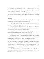
Using argument as in (De Dona et al., 2002) one can get

S
S
l
S
j
i
2
j
m
1ps
m
1pl
j
i
j
i
T
k
4
r
r
xx
Δ
⎟

⎟
⎠
⎞
⎜
⎜
⎝
⎛
>
∑
∑
+=
+=
(29)
From (24) and (29) follows
() () (){}
()
(
)
⋅+
⎪
⎩
⎪
⎨
⎧
⎥
⎦
⎤
⎢
⎣
⎡

+−⋅+ωλ+α−
∑∑
+==
Δ
m
1ps
j
i
p
1s
s
j
s
j
s
j
j
i
min
S
S
j
S
rvk1sat2vvrIExV2xV
&

Switching Control in the Presence of Constraints and Unmodeled Dynamics

235

()
{
}
(){}
2
j
i
m
1pl
j
imin
2
jii
T
ii
TT
min
11jj
2
j
S
l
s
SSS
KrIE
KRaKPBD2Q4
AAv2v
⎟
⎟
⎠

⎞
⎜
⎜
⎝
⎛
+ωλ
Δ−ω−λ
=
⎭
⎬
⎫
⎥
⎦
⎤
⎢
⎣
⎡
−Δ−⋅
∑
+=
(30)
According to relation (27) first term in (30) is always nonpositive, i.e.

()
(
)
0Vk1sat2v
s
j
s

j
S
j
≤+−
Δ
,
0k ≥∀
(31)

It is well known fact that quadratic polinomial
21
2
pzpz ++
,
1
Rz∈


is negative if zeros belong to the interval
2
2
2
11
p4pD ,
2
Dp
,
2
Dp
−=

⎟
⎟
⎠
⎞
⎜
⎜
⎝
⎛
+−−−

Using those facts it is possible to conclude that second term in relation (30) is nonpositive if
()
{}
(){}
S
S
l
S
j
2
j
i
m
1pl
j
imin
ii
T
ii
TT

min
j
KrIE
KRaKPBD2Q4
11v Δ
⎟
⎟
⎟
⎟
⎟
⎟
⎠
⎞
⎜
⎜
⎜
⎜
⎜
⎜
⎝
⎛
⎟
⎟
⎠
⎞
⎜
⎜
⎝
⎛
+ωλ

−ω−λ
++≤
∑
+=

This is true because from the definition of elipsoid
i
E fallows

[]
(
)
S
S
j
j
max
s
j
1v Δβ+≤ ,
21s
SSj ∪∈ (32)
whereby
[]
S
j
max
β is defined in the assumption A7) of Theorem.
From relation (31)-(32) follows

(
)
(
)
xV2xV α−<
&
, 0x
≠
∀
,
i
Cx
∈
,
N, ,2,1i
=
(33)
It means that closed-loop system is exponentially stable. Namely

(
)
(
)
(
)
{
}
121ej
ttexptxktx −α−≤ ,0x
≠

∀
,
i
Cx∈
(34)
whereby

{
}
{}
imin
imax
l
P
P
k
λ
λ
=
,
N, ,2,1i
=
(35)
New Approaches in Automation and Robotics

236
The trajectories in each cell
i
C
approach the origin with a exponential decrease in

()
xV
along the trajectory. According with the philosophy of control strategy, the trajectories will
enter the smallest ellipsoid corresponding to
N
ρ
. The exponential stability is assured by (33).
Remark 2. In the paper (De Dona et al., 2004) is considered the case when in the model (12)
uncertainty matrix
(
)
0wB
=
Δ
and the degree of prescribed stability 0
=
α
. Also, in that
reference the Riccati equation approach is used until in this paper the Lyapunov approach is
used.
Remark 3. When unmodeled dynamic is absent, i.e. in the Theorem 1
0a
=
,
(
)
(
)
0wEwD ==

the conditions A.5) and A.7) in the Theorem have the form
{
}
0Q
min
>
λ

[]
{}
2
j
i
m
1pl
j
i
min
N,, ,2,1i
j
max
Sl
S
Kr
Q4
1min
⎟
⎟
⎠

⎞
⎜
⎜
⎝
⎛
λ
+=β
∑
+=
=


These assumption are identical with the assumptions in reference (De Dona et al., 2002).
4. Conclusion
In this paper the switching controller with low-and-high gain and alloved over-saturation
for uncertain system is considered. The unmodeled dynamics satisfies matching conditions.
Using picewise quadratic Lyapunov function it is proved the exponential stability of the
closed loop system.
It would be interesting to develop the theory for output case and for the descrete-time case.
Also, extremely is important application of hybrid systems in distributed coordination
problems (multiple robots, spacecraft and unmanned air vehicles).
8. References
Anderson, B.D.O. & Moore, J.B. (1989). Optimal Control. Linear Quadratic Methods, Prentice-
Hall, 0-13-638651-2, New Jersey
Barmish, B.R. & Leitmann, G. (1982). On ultimate boundedness control of uncertain system
in the absence of matching conditions.
IEEE Trans. Automatic Control, Vol. 27, No. 2,
(Feb. 1982) 153-158
Blanchini, F. (1999). Set invariance in control a – survey.
Automatica, Vol.35, No. 11, (Nov.

1999) 1747-1767
Blanchini, F. & Miani, S. (2008).
Set –Theoretic Methods on Control, Birkhauser, 978-0-8176-
3255-7, Basel
Switching Control in the Presence of Constraints and Unmodeled Dynamics

237
Cassandras, C.G. & Lafortune, S. (2008). Introduction to Discrete – Event Systems, Springer
Verlag, , 978-0-387-33332-8, Berlin
De Dona. J.A., Goodwin, G.C. & Moheimani, S.O.R. (2002). Combining switching, over –
saturation and scaling to optimize control performance in the presence of model
uncertainty and input saturation.
Automatica, Vol. 38, No.11, (Nov. 2002) 1153-1162
Crama, P. & Schoukens, J. (2001). Initial estimates of Wiener and Hammerstein Systems
using multisine excitation.
IEEE Trans. Instrum Measure., vol. 50, No. 6, ( Dec. 2005)
1791-1795
Filipovic, V.Z. (2005). Performance guided hybrid LQ controller for time-delay systems.
Control Engineering and Applied Informatics. Vol. 7, No. 2, (Mar. 2005) 34-44
Goodwin, G.C., Seron, M.M. & De Dona, J.A. (2005).
Constrained Control and Estimation. An
optimization Approach
, Springer Verlag, 1-85233-548-3, Berlin
Johansson, M. (2003).
Picewise Linear Control Systems, Springer-Verlag, 3-54044-124—7, Berlin
Hippe, P. (2006).
Windup in Control, Springer Verlag, 1-84628-322-1, Berlin
Li, Z., Soh, Y. & Wen, C (2005).
Switched and Impulsive Systems. Analysis, Design and
Applications

, Springer Verlag, 3-540-23952-9, Berlin
Lin, Z., Pachter, M, Banda, S. & Shamash,Y. (1997). Stabilizing feedback design for linear
systems with rate limited actuators, In
Control of Uncertain Systems with Bounded
Inputs
, Tarbouriech, S. & Garcia, G. (Ed.), pp. 173-186, Springer Verlag, 3-540-
761837, Berlin
Lin, Z. (1999).
Low Gain Feedback, Springer Verlag, 1-85233-081-3, Berlin
Michel, A., Hou, L. & Liu, D. (2008).
Stability of Dynamical Systems: Continuous, Discontinuous
and Discrete Systems
, Birkhauser, 978-0—8176-4486-4, Basel
Ren, W. & Atkins, E. (2007). Distributed multi-vehicle coordinated control via local
information exchangle. I
nternational Journal of Robust and Nonlinear Control, Vol. 17,
No. 10-11 , (July, 2007) 1002-1033
Ren, W. & Beard, R.W. (2008).
Distributed Consensus in Multi-vehicle Cooperative Control.
Theory and Applications
, Springer Verlag, 978-1-84800-014-8, Berlin
Saberi, A., Stoorvogel, A.A. & Sannuti, P. (2000).
Control of Linear Systems with Regulation and
Input Constraints.
Springer Verlag, 1-85233-153-4, Berlin
Sun, Z. & Ge, S.S. (2005).
Switched Linear Systems. Control and Design, Springer Verlag, 1-
85233-893-8, Berlin
Tarbouriech, S. & Da Silva, J.M.G. (2000). Sinthesis of controllers for continuous – time delay
systems with saturating control via LMI’s.

IEEE Trans. Automatic Control, Vol. 45,
No. 1, (Jan. 2000) 105-111
Tsay, S.C. (1991). Robust control for linear uncertain systems via linear quadratic state
feedback,
Systems and Control Letters, Vol.15, No. 2, (Feb. 1991) 199-205
Wredenhagen, G.F. & Belanger, P.R. (1994). Picewise linear L Q control for systems with
input constraints.
Automatica, Vol.30, No. 3, (Mar. 1994) 403-416
Wu, F., Lin, Z. & Zheng, Q. (2007). Output feedback stabilization.
IEEE Trans. Automatic
Control
, Vol. 45, No. 1, (Jan. 2007) 122-128
New Approaches in Automation and Robotics

238
Zhao, W.X. & Chen, H.F. (2006). Recursive identification for Hammerstein system with ARX
subsystem.
IEEE Trans. Automatic Control, vol. 51, No. 12, (Dec. 2006) 1966-1974
14
Advanced Torque Control
C. Fritzsche and H P. Dünow
Hochschule Wismar – University of Technology, Business and Design
Germany

1. Introduction
Torque is one of the fundamental state variables in powertrain systems. The quality of
motion control highly depends on accuracy and dynamics of torque generation. Modulation
of the air massflow by opening or closing a throttle is the classical way to control the torque
in gasoline combustion engines.
In addition to the throttle and the advance angle several other variables are available to

control the torque of modern engines - either directly by control of mixture or indirectly by
influence on energy efficiency. The coordination of the variables for torque control is one of
the major tasks of the electronic control unit (ECU).
In addition to the generation of driving torque other objectives (emission threshold, fuel
consumption) have to be taken into account. The large number of variables and pronounced
nonlinearities or interconnections between sub-processes makes it more and more difficult
to satisfy requirements in terms to quality of control by conventional map-based control
approaches. For that reason the investigation of new approaches for engine control is an
important research field (Bauer 2003).
In this approach substitute variables instead of the real physical control variables are used
for engine torque control. The substitute variables are used as setpoints for subsidiary
control systems. They can be seen as torque differences comparative to a torque maximum
(depending on fresh air mass). One advantage of this approach is that we can describe the
controlled subsystems by linear models. So we can use standard design methods to
construct the torque controller. Of course we have to consider variable constraints. Due to
the linearization the resulting control structure can be used in conventional controller
hardware.
For the superordinate controller a Model Predictive Controller (MPC) based on state space
models is used because with this control approach constraints, and also setpoint- and
disturbance progressions respectively, are considered.
In chapter 2 we briefly explain the most important engine processes and the main torque
control variables. The outcome of this explanations is the use of a linear multivariable model
as a bases for the design of the superordinate torque controller. The MPC- algorithm and its
implementation are specified in chapter 3. Chapter 4 contains several examples of use.
In this chapter it is also shown how the torque controller can change to a speed- or
acceleration controller simply by manipulation of some weighting parameters.
New Approaches in Automation and Robotics

240
2. Process and torque generation

Combustion and control variables: In figure 1 the four cycles of a gasoline engine are
shown in a pressure/volume diagram. The mean engine torque results from the difference
energy explained by the two closed areas in the figure.
The large area describes the relation of pressure and volume during compression and
combustion. The charge cycle is represented by the smaller area.
For good efficiency the upper area should be as large as possible and the area below should
be minimal (for a given gas quantity). The best possible efficiency in theory is represented
by the constant-volume cycle (or Otto cycle) (Grohe 1990, Urlaub 1995, Basshuysen 2002).


Fig. 1. p-V-Diagram (gasoline engine)
The maximum torque of the engine basically depends on the fresh air mass which is
reaching the combustion chamber during the charge cycle. A desired air/fuel mixture can
be adjusted by injecting an appropriate fuel quantity. The air/fuel-ratio is called lambda (λ).
If the mass of fresh air corresponds to the mass of fuel (stoichiometric ratio) the lambda
parameter is one (λ=1). By several reasons the combustion during the combustion cycle is
practically never complete. So after the cycle there remain some fresh air and also unreacted
particles of fuel. A more complete reaction of the air can be reached by increasing fuel mass
(λ<1). This results in rising head supply and hence to an increase of the potential engine
torque. The maximum of torque is reached by approximately λ=0.9. The torque decreases
more and more if lambda increases. So one can realize fast torque changes for direct
injection engines by modulation of the fuel.
The maximum of lambda is bounded by combustibility of the mixture (depends on
operating conditions). For engine concepts with lean fuel-air ratio (λ>1) the fuel feed is the
main variable for torque control. Because of the exhaust after treatment λ=1 is requested for
most gasoline engines at present. In case of weighty demands however it is possible to
change lambda temporary.
Advanced Torque Control

241

In addition to air and fuel the torque can be controlled by a number of other variables like
the advance angle or the remaining exhaust gas which can be adjusted by the exhaust gas
recirculation system.
For turbocharged engines the air flow depends in addition to the throttle position on
turbocharger pressure which can be controlled by compressors or by exhaust gas turbines.
Pressure charging leads to an increase of the maximum air mass in the combustion chamber
and hence to an increasing maximum of torque even if the displaced volume of the engine is
small (downsizing concepts).
Because of the mass inertia of the air system it takes time until a desired boost pressure is
achieved. The energy for the turbocharging process is taken from the flue gas stream. This
induces a torque load which can result in nonminimumphase system behaviour.
In addition to the contemplated variables there are further variables imaginable which
influence the torque (maximum valve opening, charge-motion valve, variable compression
ratio, etc.).
Furthermore the total torque of the engine can be influenced by concerted load control. For
example one can generate a negative driving torque by means of the load of the electric
generator. The other way around one can generate a fast positive difference torque by
abrupt unloading. This torque change can be much faster than via throttle control.
In hybrid vehicles we have a number of extra control variables and usable parameters for
torque control.
More details on construction and functionality of internal combustion engines are described
by Schäfer and Basshuysen 2002, Guzella and Onder 2004 and Pulkrabeck 2004.
For control engineering purposes the torque generation process of a gasoline engine is
multivariable and nonlinear. It has a large number of plant inputs, a main variable to be
controlled (the torque) and some other aims of control like the quality of combustion
concerning emission and efficiency.
Considerable differences in the dynamic behaviour of the subsystems generate further
problems particularly for the implementation of the control algorithms. For example we can
change the torque very fast by modulation of the advance angle (compared to the throttle).
Normally the value that causes the best efficiency is used for the advance angle. However to

obtain the fastest torque reduction it can be helpful to degrade the efficiency and so the
engine torque is well directed by the advance angle. Fast torque degradation is required e. g.
in case of a gear switching operation. For the idle speed control mode fast torque
interventions can be useful to enhance the stability and dynamics of the closed loop. Fast
load changes also necessitate to generate fast torque changes. In many cases the dynamic of
sub-processes depends on engine speed and load.
Whether the torque controller uses fast- or slow-acting variables depends on dynamic,
efficiencies and emission requirements. Mostly the range of the manipulated variables is
bounded.
In the normally used "best efficiency" mode one can only degrade the torque by the
advanced angle. For special cases (e. g. idle speed mode) the controller chooses a concerted
permanent offset to the optimal advance angle. So a "boost reserve" for fast torque
enhancement occurs. Because of the efficiency this torque difference is as small as possible
and we have a strong positive (and changeable) bound for the control variable. This should
be considered in the control approach. The main target variables and control signals are
pictured in figure 2.
New Approaches in Automation and Robotics

242
We can summarize: The torque control of combustion engine is a complex multivariable
problem. In addition to the torque we have to control other variables like lambda, the
efficiency, EGR , etc. The sub-processes are time variant, nonlinear and coupled. The control
variables are characterized by strong bounds.


Fig. 2. Actuating and control variables
Torque control: Below we describe the most important variables for torque control and the
effect chain.
a.) fresh air mass:
As aforementioned the engine torque mainly depends on the fresh air mass as the base for

the maximum fuel mass. Classical the air mass is controlled by a throttle within the intake.
In supercharged engines the pressure in front of the throttle can be controlled by a
turbocharger or compressor. The result of supercharging is a higher maximum of fresh air
mass in the combustion chamber. This leads to several benefits. In addition to the throttle or
charging pressure the air mass flow can also be controlled by a variable stroke of the inlet
valve.
It is not expedient to use all variables of the air system for torque control directly. For the
torque generation the air mass within the cylinder is mainly important (not the procedure of
the adjustion). Hence it is more clever to use the setpoint for the fresh air mass as the plant
input for the torque controller. This can be realized by the mentioned control variables with
a the aforementioned sub-control system. One advantage of the approach is, that the sub-
control system at large includes measures for the linearization of the air system.
Furthermore the handling of bounds is a lot easier in this way.
b.) exhaust gas recirculation (EGR):

By variable manipulating of the in- and outlet valves it is possible to arrange, that both
valves are simultaneously open during the charge cycle (valve lap). So in addition to the
fresh air some exhaust gas also remains the combustion chamber. This is advantageous for
the combustion and emission. In case of valve lap the throttle valve must be more open for
the same mass of fresh air. This is another benefit because the wastage caused by the throttle
decreases. The EGR can also be realized by an extern return circuit. Here we only consider
the case of internal EGR. The EGR induced a deviation from the desired set point of fresh
air. This deviation usually will be corrected by a controller via the throttle. As
aforementioned this correction is relatively slow. If the mechanism for the valve lap allows
fast shifting we can realize fast torque adjustments because the change of air mass by the
valve lap occurs immediately.
Advanced Torque Control

243
c.) advance angle:

An important parameter for the efficiency of the engine is the initiation of combustion. The
point of time mainly depends on the advance angle. The ignition angle which leads to the
best efficiency is called the optimized advance angle. It depends on engine speed and the
amount of mixture. A delay in the advance angle leads to less efficiency and to the decrease
of engine torque. The relation between advance angle and torque is nonlinear.
d.) lambda:

The amount of fuel determines (for a given fresh air mass) the torque significantly. As
aforementioned bounded we can manipulate the torque by lambda. For direct injection
concepts the torque changes immediately if lambda is modified. Torque control by means of
lambda is limited for engine concepts with λ=1.
e.) other variables

The quality of mixture has also an effect on the efficiency and so on the torque. For the
quality several construction parameters are important. Further the quality depends on
adjustable variables like fuel pressure, point of injection or the position of a charge-motion
valve. The setpoints for these parameters are primarily so chosen that we obtain best
mixture efficiency.
In figure 3 the main variables and the effects on the process are outlined.


Fig. 3. Main variables to influence the energy conversion and the torque generation
From the explanation up to now we can deduce appropriate variables for torque control:
− fresh air mass in the combustion chamber (adjustable via charge pressure, throttle,
valve aperture and valve lap),
− fuel, lambda (adjustable by injection valve),
− advance angle,
− internal exhaust gas recirculation (adjustable via valve lap)
All variables are bounded.

Subsidiary control systems: For simplification of the torque control problem it is expedient
to divide the process in to several sub-control circuits. The following explanations are aimed
New Approaches in Automation and Robotics

244
to gasoline engines with turbo charging, internal EGR, direct injection and homogeneous
engine operation (λ=1).
The sub-control circuits are outlined in figure 4. The most complicated problem is the design
of the subsystem for fresh air control. Because of the strong connection of fresh air and EGR
it makes sense to control both simultaneously in one sub-system. The control system has to
consider or compensate a number of effects and nonlinear dependences.
The main task is to control the fresh air mass and the desired amount of exhaust gas which
reaches the combustion chamber during the charge cycle. The control system should reject
disturbances and adjust new setpoint values well (fast, small overshoot). Another
requirement is that it should be possible to describe the complete control circuit by a linear
model.
For the control structure we propose a reference-model controller (figure 5). One of the aims
of this control structure is to achieve a desired dynamic behaviour for the circuit. The
mentioned requirement for simplification of the modelling is implicitly given in this way.
Nonlinear effects can be compensated by appropriate inverted models.


Fig. 4. Model Following Control (MFC)
In the explained approach the fresh air mass is used as the main control variable. From this
air mass results the maximum possible torque with approximately λ = 0.9.
In case of modification of the exhaust gas portion we only consider the influence on the
fresh air. The influence on combustion quality is disregarded. Increasing of exhaust gas
portion leads to decreasing of fresh air and so to reduction of torque. This influence is
compensated by a special controller so that the action of EGR on the engine torque is
comparable to the characteristic of a high-pass filter. An advantage is obtained if the acting

effect from EGR-setpoint to the fresh air is faster than via the throttle. In this case it is
possible to realize fast (but transient) changes of the torque.
For torque manipulation via the advance angle it is not necessary to use a feedback system.
The influence on the efficiency of the engine can be modelled by a characteristic curve. So
for this control path a feedforward control action is adequate. We can find the same
conclusion for lambda.
Second-level control system: By means of the described sub-control systems the actuating
variables of the torque control system can be defined. The main variables are the setpoints of
the fresh air mass, the exhaust gas, the advance angle and the setpoint for lambda. The
relation between the torque and the mentioned variables is nonlinear. Following the torque
controller also had to be nonlinear and the controller design could be difficult.
A more convenient way is to linearize the sub-control systems first by stationary functions
at the in and outputs. In the described control approach the control variables are substituted
by a number of partial torque setpoints (delta torques). The partial torques represent the
Advanced Torque Control

245
influence of the used control variables to the whole engine torque. The over-all behaviour of
the system to be controlled is linear (widely).
Base control variable is the theoretical maximum of the torque for a given fresh air mass.
The other variables can be seen as desired torque differences to a reference point (the
maximum of torque). That means if the delta variables all set to zero, the maximum of
torque for the given fresh air mass should be generated by the engine.
The difference variables are both: actuation variables for the torque and variables to be
controlled. In this way it is possible to adjust stationary other setpoints for lambda, the
residual exhaust gas or the advance angle.
We can find the bounds for the substituted variables from the physical bounds also by using
the linearization functions. It is assumed that the nonlinear functions are monotone in the
considered range.
From the explanations above the total control structure follows (figure 5). The plant for the

torque controller consists of the sub-control-systems (fresh air, residual exhaust gas, and
lambda and advance angle) and the stationary linearization systems. The whole system can
be described by a linear multivariable model. Only the bounds of the input variables have to
be taken into account. The plant outputs are the engine torque and the difference variables.
Other plant outputs could be estimated values for exhaust gas emission or for fuel
consumption (can be estimated by simplified models).
The setpoints for the torque are generated by the driver or by other ECU-functions (e.g. for
changing gears). For the realization one can find different requirements.
For example we have to realize a requested torque as fast as possible. For other situations
the time could be less important and one wish to realize a desired torque with a minimum
of consumption. The control system should be able to handle all the different requirements.
The control variables are not available at all time. In general the range of the control
variables is bounded. Sometimes they may not differ from the setpoint. The torque
controller should consider this variability of bounds.
An appropriate control principle with the ability to solve this problem is the well known
model predictive controller (MPC). This approach can handle variable bounds as well as
known future setpoints and disturbances. Future setpoints are known for instance for
changing gears. Switch-on of the air conditioning system is an example for known future
disturbances. Matching to miscellaneous priorities is possible by appropriate weighting
matrices in the control algorithm.
The model structures for the superordinate torque control system can be explained from
figure 5.
For example we can arrange the model equation

⎥
⎥
⎥
⎥
⎦
⎤

⎢
⎢
⎢
⎢
⎣
⎡
⋅
⎥
⎥
⎥
⎥
⎦
⎤
⎢
⎢
⎢
⎢
⎣
⎡
=
⎥
⎥
⎥
⎥
⎦
⎤
⎢
⎢
⎢
⎢

⎣
⎡
4
3
2
1
44
33
22
14131211
4
3
2
1
)(000
0)(00
00)(0
)()()()(
u
u
u
u
sG
sG
sG
sGsGsGsG
y
y
y
y

(1)
if we use all of the aforementioned control variables (fresh air, residual exhaust gas, lambda
and advance angle). The output signals of the model are the engine torque (y
1
) and the three
difference control variables which appear in fact (y
2
… y
4
).
New Approaches in Automation and Robotics

246

Fig. 5. Two layer control approach
The engine torque (y
1
) depends on all actuating variables. G
11
(s) describes the effect of the
fresh air path to the engine torque, G
12
(s) models the effect of the exhaust gas path on the
engine torque, G
13
(s) describes the behaviour of the torque depending on lambda and G
14
(s)
the effect of the ignition angle path. We may assume, that the output variables y
2

y
4
are
only dependent on the corresponding setpoints because of the decoupling effects of the sub-
control circuits. G
22
(s), G
33
(s) and G
44
(s) are simple low-order transfer functions.
If we have (in addition to the torque setpoint) other control requirements (e.g. consumption)
it is easy to extend the model by appropriate transfer functions for the estimation of the
control variable effects on the considered output variables. For exhaust gas emission and
fuel consumption this results in a model as follows:

⎥
⎥
⎥
⎥
⎦
⎤
⎢
⎢
⎢
⎢
⎣
⎡
⋅
⎥

⎥
⎥
⎥
⎥
⎥
⎥
⎥
⎦
⎤
⎢
⎢
⎢
⎢
⎢
⎢
⎢
⎢
⎣
⎡
=
⎥
⎥
⎥
⎥
⎥
⎥
⎥
⎥
⎦
⎤

⎢
⎢
⎢
⎢
⎢
⎢
⎢
⎢
⎣
⎡
4
3
2
1
64636261
54535251
44
33
22
14131211
6
5
4
3
2
1
)()()()(
)()()()(
)(000
0)(00

00)(0
)()()()(
u
u
u
u
sGsGsGsG
sGsGsGsG
sG
sG
sG
sGsGsGsG
y
y
y
y
y
y
(2)
The extension of the model is possible by using any other variable of the engine as plant
output signals. Possibilities are, for instance, the engine speed or the acceleration.
Advanced Torque Control

247
In this way we can consider the torque and the speed simultaneously. The model has to be
completed to:

.
)()()()(
4

747372717
⎥
⎦
⎤
⎢
⎣
⎡
⋅
⎥
⎦
⎤
⎢
⎣
⎡
=
⎥
⎦
⎤
⎢
⎣
⎡
u
sGsGsGsGy
M
MMMMM
(3)
y
7
describes the engine speed. The transfer functions of the lower line describe the effects of
all inputs on the speed.

Certainly, it is not possible to adjust torque and speed independently. The structure allows
however to switch between torque and speed control smoothly. This can be done by the
weighting parameters of the MPC. In the same way it is feasible to extend the model by a
line which describes the acceleration depending on the input signals. A disadvantage of the
model extensions is the increasing complexity.
3. MPC-algorithm and implementation
3.1 Approach
As mentioned the model predictive control concept seems to be an appropriate approach for
torque control. In the following we describe the basics of this control concept. The
explanations are focused mainly on a state space solution.
MPC is widely adopted in industries, primarily in chemical engineering processes. This
control principle is an established method to deal with large constrained multivariable
control problems (Dittmar 2004, Dünow 2004, Grimble 2001, Maciejowsky 2002, Salgado et
al. 2001). The main idea of MPC is to precalculate the control action by repeatedly solving of
an optimization problem (see figure 6). The optimization aims to minimize a performance
criterion during a time-horizon subject to selected control and plant signals. An appropriate
and usual criterion is the quadratic cost function
∑∑
=
−
=
+Δ+Δ++−++−+=
p
u
H
i
H
i
i
T

i
T
kikuRkikuikrkikyQikrkikykJ
0
1
0
).|(
ˆ
)|(
ˆ
))()|(
ˆ
())()|(
ˆ
()(

(4)
)|(
ˆ
kiky +
denotes the predicted output for the time
ik
+
calculated at the time instant
k
.
u
ˆ
Δ
denotes the difference control signal. Q and R are the weighting matrices for the input

and the output variables of the process. H
p
and H
u
are prediction and control horizons. The
use of difference control signals for the cost function leads to better control structuring and
inhibits high-frequency signals. Unlike huge computing potential in other application fields
of MP-Controllers the hardware capacity of engine control systems is limited in memory
and computing power. For this reason we implemented a MPC-algorithm which is suitable
for realtime application in engine control units. As minimum requirements the control
algorithm should allow the application to multivariable systems with variable constraints in
the control output. A main design requirement was the achievement of reasonable
computing efforts.
For the MP-Controller we use a set of linear constant time-discrete state-space process
models of the form
New Approaches in Automation and Robotics

248

)()(
)()()1(
kCxky
kBukAxkx
=
+
=
+
(5)
(u-input signal, y-output signal, x-state of the system, A-system matrix, B-input- and C-
output matrix).

Fig. 6. Predictive Control: The basic idea
In case of control signal constraints we have to consider the conditions

)1()|1()1(
)1()|1()1(
)()|()(
maxmax
maxmin
maxmin
−+≤−+≤−+
+≤+≤+
≤≤
uuu
HkukHkuHku
kukkuku
kukkuku
MMM
(6)
From the model we obtain the prediction for the output of the system for a horizon of
p
H

steps at time
k .
⎥
⎥
⎥
⎥

⎦
⎤
⎢
⎢
⎢
⎢
⎣
⎡
−+Δ
+Δ
Δ
⎥
⎥
⎥
⎥
⎥
⎥
⎥
⎥
⎥
⎥
⎥
⎥
⎦
⎤
⎢
⎢
⎢
⎢
⎢

⎢
⎢
⎢
⎢
⎢
⎢
⎢
⎣
⎡
+
+
+−
⎥
⎥
⎥
⎥
⎥
⎥
⎥
⎥
⎥
⎥
⎦
⎤
⎢
⎢
⎢
⎢
⎢
⎢

⎢
⎢
⎢
⎢
⎣
⎡
+
⎥
⎥
⎥
⎥
⎥
⎥
⎥
⎥
⎦
⎤
⎢
⎢
⎢
⎢
⎢
⎢
⎢
⎢
⎣
⎡
=
⎥
⎥

⎥
⎦
⎤
⎢
⎢
⎢
⎣
⎡
+
+
∑∑
∑
∑
∑
∑
∑
−
=
−
=
=
−
=
−
=
=
−
=
+
)|1(

ˆ
)|1(
ˆ
)|(
ˆ
)(
0)(
0
)1()(
)|(
ˆ
)|1(
ˆ
0
1
0
0
1
0
1
0
0
1
0
1
kHku
kku
kku
BACBAC
BABCBAC

CBBAC
BABC
CB
ku
BAC
BAC
BAC
CB
kx
CA
CA
CA
CA
kHky
kky
u
HH
i
i
H
i
i
H
i
i
H
i
i
H
i

i
H
i
i
H
i
i
H
H
H
p
upp
u
u
p
u
u
p
u
u
M
L
MMM
L
L
MOM
L
L
M
M

M
M
M

(7)

)()1()()( kUkukxky
Θ
Δ
+
−
Υ
+
Ψ
=
=
(8)
Advanced Torque Control

249
With the setpoint signal
)|( kikr
+
,
p
Hi K0
=
, the equation
)1()(
)|(

)|1(
)|(
)( −Υ−Ψ−
⎥
⎥
⎥
⎥
⎥
⎦
⎤
⎢
⎢
⎢
⎢
⎢
⎣
⎡
+
+
= kukx
kHkr
kkr
kkr
k
p
M
ε

(9)
and the weight matrices

⎥
⎥
⎥
⎥
⎦
⎤
⎢
⎢
⎢
⎢
⎣
⎡
−
=
⎥
⎥
⎥
⎥
⎥
⎦
⎤
⎢
⎢
⎢
⎢
⎢
⎣
⎡
=
)1(000

0)1(0
00)0(
)(00
0)1(0
00)0(
u
p
HR
R
R
Rlyrespective
HQ
Q
Q
Q
MOMM
L
L
L
MOMM
L
L

(10 and 11)
the cost functional (4) becomes to

)()()( kUHUGkUkJ
TT
ΔΔ+Δ−=
(12)

with

RQHandkQG
TT
+ΘΘ=Θ= )(2
ε
(13 and 14)
The constraint conditions from equation 6 we can formulate as a linear matrix inequation
like

int
)(
constra
UkUA
≤
Δ
(15)
with
⎥
⎥
⎥
⎥
⎥
⎥
⎥
⎥
⎥
⎥
⎥
⎦

⎤
⎢
⎢
⎢
⎢
⎢
⎢
⎢
⎢
⎢
⎢
⎢
⎣
⎡
−+−+−
−++−
−+−
−−−+
−−+
−−
=
⎥
⎥
⎥
⎥
⎥
⎥
⎥
⎥
⎥

⎥
⎥
⎦
⎤
⎢
⎢
⎢
⎢
⎢
⎢
⎢
⎢
⎢
⎢
⎢
⎣
⎡
−−−−
−−
−
=
)1()1(
)1()1(
)1()(
)1()1(
)1()1(
)1
()(
1111
0011

0001
1111
0011
0001
min
min
min
max
max
max
int
kuHku
kuku
kuku
kuHku
kuku
kuku
UandA
u
u
constra
M
M
L
MOMMM
L
L
L
OMMM
L

L

(16 and 17)
The main problem of the model predictive controller is to minimize the cost function 12
subject to the constraints expressed in inequation 15. To solve this standard convex
optimization problem (which is summarized in figure 7) efficient numerical procedures
(quadratic programming (QP)) are available. For the realtime application we developed a
computing time optimized QP program which uses an active set algorithm (Dünow et al.
2005, Lekhadia et al. 2004, Lekhadia 2004a). We implemented this optimization algorithm
New Approaches in Automation and Robotics

250
for Mathworks xPC-Target and for an Infineon TriCore microcontroller board. This
microcontroller is actually also used in ECU-Systems.
Fig. 7. MPC-algorithm (summarized)
3.2 Implementation
The model predictive controller was implemented by means of the packages LAPACK and
BLAS for C-language (Dünow et al. 2005). These Libraries are efficient concerning the
computing effort and widely used in research and industrial applications. The MPC-
algorithm was implemented by a C-S-function for Matlab / Simulink to use it on a xPC
Target system. Because of the limited capabilities of the ECU the implemented control
algorithm should need less computing time and memory space. For the unconstraint case
we can find a constant MPC solution. Here the bounds will be ignored. The optimal
)(kUΔ

for the unconstrained case we find by

0)(2)/(
)(
=

Δ
+
−
=
∇
=
Δ
Δ
kUHGJUddJ
kU
(18)
From equation 18 follows the optimal set of control variables:

GHkU
opt
1
2
1
)(
−
=Δ
(19)
Condition 16 minimizes the cost function because of the fact that

(
)
RQH
kU
J
T

+ΘΘ⋅==
Δ∂
∂
22
)(
2
2
(20)





Standard Problem Quadratic Programming
)()()()( kUHkUGkUkJ
TT
ΔΔ+Δ−=
Essential Parameters:
Hp, Hu : Prediction and Control Horizon
Q, R : Weighting Matrices
SP : Setpoint
X : States
U : Inputs
Cnstr. : Constraints
Model : Model of the plant

H, G, A, U
constraints

Active Set

Methods
Min.
UkUA
≤
Δ
)(
Constraints
Advanced Torque Control

251
is positive defined if
0≥Q
and
0>R
. In figure 8 the unconstrained case is summarized in
a block diagram. The implementation of a controller which based on equation 19 is outlined
in figure 9. Here the controller consists of a linear state space model, three constant gains
and a simple wind up clipping structure (Dünow et al. 2005).

Fig. 8. Block diagram of the unconstrained case

Fig. 9. Implementation of the constant Controller in Matlab/Simulink (Dünow et al. 2005)
For the constrained case we have to minimize the cost function (see equation 12) regarding
to the controller constraints output marked in equation 15. With the help of active set
methods we solved this standard quadratic programming optimization problem. In figure
10 the flow chart, which based on Fletscher 1997, Gill et al. 1991 and Maciejowski 2002, of
the optimization algorithm is shown. The active set method involves two phases. At first a
feasible point is calculated. The second phase involves the generation of an iterative
sequence of feasible points that converge to the solution. The λ-check below in figure 10 is a
test for Karush-Kuhn-Tucker condition for a global optimum (Fletscher 1987).

New Approaches in Automation and Robotics

252

Fig. 10. Flow chart of the implemented active set algorithm (Dünow et al. 2005 and Lekhadia
2004a)
4. Practical applications and results
In this section we will investigate practical aspects of the described approach. As a test
environment we used a complex nonlinear model of a four-cylinder direct injection engine.
This model includes the physical elements of the engine as well as the necessary ECU-
functions for torque control. The model is usable at Matlab/Simulink. The model is briefly
depicted in figure 11.
Search Direction
(
)
(
)
[
]
⎭
⎬
⎫
⎩
⎨
⎧
Δ
−
=
−=Δ=
uA

cnstr
gZHZZZuSD
i
i
k
T
k
T
k
T
k
T
k
min
α

where i = 1…m
and GSD = A
i
Δu

>

0
So
uuu
k
k
Δ
+

=
+
α
1


False
False
True
Find Initial feasible solution
A
i
= []; Initially no active constraints
u
k
= 0; where [m, n] = size(A
i
)
Z
k
= 1;
GHug
buAconstr
kk
iki
+=
−
=

Check if

λ
is negative
[,] ( )
(\( ))
i
T
ik
QR qrA
RQg
λ
=
=−

If

0
i
λ
≥

Then
1
+
k
u is Optimal and Minimum
Add the blocking constraints
in Active-Set
i
A

Remove that active constraint from
Active-Set
i
A
(,:)
[,] ( )
[,] ( )
[:, 1: ]
i
i
i
k
AAi
Q R qr A
mn sizeA
Z
Ql m
=
=
=
=+

l
= no. of active constraints
GHug
buAcnstr
kk
iki
+=
−

=

True
If α ≥ 1 & No
constraint violation
Then
1
+
k
u
is an optimal solution
Advanced Torque Control

253


Fig. 11. Engine model (simplified)
The model was completed by a part for exhaust gas emission and one part for fuel
consumption.
Because of the different dynamics of the control pathways the sampling time is relatively
small. This results in a corresponding large prediction horizon of the MPC. Regarding the
control horizon we btained the best compromise between performance and computational
effort for H
u
= 5.
Figure 12 foreshadows the structure of the simulation system. We used a state space method
for the modelling and solution of the control problem. The MPC-Block in the left of the
simulink-model includes the control solution explained in section 3. The process model can
be seen as an alternative to a real engine. The background of the model was illustrated in
section 1 and 2. The model in the controller block is conform to equation 2.

a) MPC and engine process b) Optimization and internal model

Fig. 12. Simulation environment
New Approaches in Automation and Robotics

254
In figures 13a to 13d an application case of the torque controller is shown. The main
objective of the control process in this example is to follow the torque setpoint as accurately
as possible. The upper figure (13a) shows the setpoint and the real values of the torque.
Below (13a) the four control variables are pictured. At about 1.5 seconds we have a setpoint
step. At 2.5 seconds a load step occurs. This load step is predictable (turn-on procedure of
the air conditioner). In the example the setpoints for the delta torques of the ignition and
exhaust gas path are zero. The setpoint for the lambda torque path is here about -8 Nm. This
corresponds to λ=1. The torque value of 8 Nm can be seen as a "reserve" and the MPC can
boost the total engine torque due to the fuel path immediately by this value. The upper
bound for the delta torque via the fuel path is zero in the example.
1 2 3 4 5 6 7
-5
0
5
10
15
Time in s
Torque in Nm

1 2 3 4 5 6 7
-20
-10
0
10
20
30
Time in s
Torque in Nm


Torque (fresh air)
Torque (exhaust gas)
Torque (ignition angle)
Torque (lambda)
Torque setpoint
Torque

Fig. 13a. Results – max torque priority
The upper and lower bounds for the exhaust gas path in the example are equal (zero). That
means the MPC must not use this variable for torque control until the constraints are
changing. The value of the controller output always is equal to the setpoint (as required).
Because of the fact that the controller outputs for the delta torques at the same time are
variables to be controlled these outputs are used only temporarily by the MPC (also visible
in figure 13b). The lower bounds for the fuel and the ignition path in the example are -15
Nm. The setpoint step for the total engine torque at 1.5 seconds was predictable. It is visible
that the MPC automatically prepared this action. The maximum torque (represented by the
air path) increases. The available delta variables (fuel and ignition path) are decreasing. So
the total torque doesn't change up to 1.5 seconds. In this way the MPC builds up a torque
reserve which can be used (temporarily) to advance the setpoint adjustment.

The compensation of a predictable load step (in the example about at 2.5 seconds) occurs in
the same way. Figure 13b and 13d give a zoomed view to the load compensation. The
controller is able to readjust the torque very fast due to the torque reserve.
Advanced Torque Control

255
2.1 2.2 2.3 2.4 2.5 2.6 2.7 2.8 2.9 3
0
1
2
3
4
5
6
Time in s
Torque in Nm


2.1 2.2 2.3 2.4 2.5 2.6 2.7 2.8 2.9 3
-10
0
10
20
30
Time in s
Torque in Nm


Torque (fresh air)
Torque (exhaust gas)

Torque (ignition angle)
Torque (lambda)
Torque s et point
Torque

Fig. 13b. Results – max torque priority
In the example above the control request was focused mainly to minimize the engine torque
deviation from the desired setpoint. This was achieved by appropriate weighting variables
within the model predictive control algorithm.

1 2 3 4 5 6 7
-5
0
5
10
15
Time in s
Torque in Nm


1 2 3 4 5 6 7
-10
0
10
20
30
Time in s
Torque in Nm

Torque (fresh air)
Torque (exhaust gas)
Torque (ignition angle)
Torque (lambda)
Torque setpoint
Torque

Fig. 13c. Results – min torque priority
New Approaches in Automation and Robotics

256
By changing the weighting factors it is also possible to shift the focus more towards other
attributes. For instance one can achieve a reduction of the waste gas emission by a setpoint
for corresponding λ=1 and increasing the weighting factors of the lambda path.
The results are shown in figure 13c for the same setpoint and load steps as in the example
above. It is visible that the torque adjustment is (compared to figure 13a) slower and the
controller output for the fuel path is used only marginally.

2.1 2.2 2.3 2.4 2.5 2.6 2.7 2.8 2.9 3
0
1
2
3
4
5
6
Time in s
Torque in Nm

2.1 2.2 2.3 2.4 2.5 2.6 2.7 2.8 2.9 3
-10
0
10
20
30
Time in s
Torque in Nm


Torque (fresh air)
Torque (exhaust gas)
Torque (ignition angle)
Torque (lambda)
Torque s et point
Torque


Fig. 13d. Results – min torque priority
As mentioned in section 2 the described control approach allows to switch smoothly
between torque, speed or acceleration control. This can be simply achieved by the model
extension (described in section 2, equation 3) and appropriate weighting parameters for the
MPC. Only by shifting the weighting factors one can switch from speed control to torque
control and back.
The plots in figure 14 demonstrate how this control mode works. In this example we used
only the fresh air and the ignition path for torque control. Up to 3 seconds the controller
should work as a speed controller. From then it should work as a torque controller. At
approximately 6 seconds the weighting factors where switched back to speed control mode
values. Equation 21 represents the linear model which is used internally by the MPC for this
example.

⎟
⎟
⎠
⎞
⎜
⎜
⎝
⎛
Δ
⋅
⎟
⎟
⎟
⎠
⎞
⎜
⎜
⎜
⎝
⎛
=
⎟
⎟
⎟
⎠
⎞
⎜
⎜

⎜
⎝
⎛
Δ
Setpoint Anglegnition
SetpointAir Fresh
32
2221
1211
AngleIgnition
)(0
)()(
)()(
Speed Engine
Torque Engine
I
Torque
Torque
sG
sGsG
sGsG
Torque
(21)
Advanced Torque Control

257
Switching between speed and torque control can simply be realized by changing some
weighting factors. The behaviour of the MPC changes automatically. This is a very
convenient way to change for instance to the idle speed control mode and back to torque
control.

In figure 14 first the speed control is active. The speed follows the desired characteristic
whereas the torque is different from the corresponding setpoint. After changing the
weighting factors the torque will be adjusted to the setpoint and the engine speed is only
marginally considered by the controller.

Time period in
s
Active
Control
Torque weighting
factor
Speed weighting
factor
0 … 2.5 Speed control 0 1
2.5 …6
Torque
control
1 0
6 … 8.5 Speed control 0 1

Table 1. Enabled control

0 1 2 3 4 5 6 7 8
800
900
1000
1100
Time in s
Speed in rpm

0 1 2 3 4 5 6 7 8
-8
-6
-4
-2
0
2
Time in s
Torque in Nm


0 1 2 3 4 5 6 7 8
0
10
20
30
Time in s
Torque in Nm


0 1 2 3 4 5 6 7 8
0
2
4
6
Time in s
Torque in Nm

Load Torque
Torque about Fresh Air
Torque about Ignition Angle
Torque Setpoint
Torque
Speed Setpoint
Speed


Fig. 14. Speed and Torque Control