Challenges and Paradigms in Applied Robust Control Part 9 pps
Bạn đang xem bản rút gọn của tài liệu. Xem và tải ngay bản đầy đủ của tài liệu tại đây (1.29 MB, 30 trang )
Discussion on Robust Control Applied to Active Magnetic Bearing Rotor System 23
0
1
23
4
5
−150
−100
−50
0
50
100
150
Time, s
Displacement, μm
2
4
6
8
10
Speed, ×1000 rpm
(a) Robust H
∞
controller
0
1
23
4
5
−150
−100
−50
0
50
100
150
Time, s
Displacement, μm
2
4
6
8
10
Speed, ×1000 rpm
(b) LPV controller
Fig. 16. Rotor acceleration responses.
point of 6500 rpm where the system crosses the first flexible mode. The second point where
the system experiences oscillations is close to the maximum speed and it can be explained by
the deceleration of the rotor. The LPV controller has a lower magnitude of oscillations around
this point; the difference is 35 %. Such a behavior can be explained by an adaptive nature
of an LPV controller. In each step, the gains are modified according to the rotational speed.
During the acceleration process, the system does not have enough time to adapt. This results
in a higher amplitude of oscillations. During the later deceleration phase, the coefficients
do not change that fast and performance is better. The speed of the parameter variation is
a significant problem for the LPV controllers, and usually the main point of conservatism in
that approach (Leith & Leithead, 2000).
The second simulation experiment in the steady state proves that LPV controller provides
a better performance. In this experiment, a step disturbance to the x channel of the rotor
A-end is applied at the maximum rotational speed. The simulation results are presented
in Fig. 17. The magnitude of the disturbance response for an LPV controller is about three
times smaller than that of a robust controller. Additionally, the LPV controller does not have
coupling between different ends, so the disturbance does not propagate through the system.
6. Real-time operating conditions
The AMB-based system requires hard-real time controllers. In the case of a robust control
strategy, the control law is of higher complexity than other solutions. Therefore, the
implementation of the control law must fulfill the requirements of the target control system
such as finite precision of the arithmetic and number format and available computational
229
Discussion on Robust Control Applied to Active Magnetic Bearing Rotor System
24 Will-be-set-by-IN-TECH
0 0.05
0.1 0.15
0.2 0.25 0.3
0
100
200
300
Time, s
Displacement, μm
LPV End A
LPV End B
Robust End A
Robust End B
Fig. 17. Step disturbance response for controllers in the x direction.
power. The digital control realization requires a digital controller that matches the continuous
form in the operating frequency range. The controllers for the radial suspension of the AMB
rotor system are tested using a dSpace DS1005-09 digital control board and a DS4003 Digital
Input/Output system board as a regulation platform. The Simulink and Real-time Workshop
software are applied for automatic program code generation. The selected sampling rate is
10 kHz. The resolution of the applied ADCs is 16 bits. The control setup limits the maximum
number of states of the implemented controllers to 28 states.
7. Conclusions
The chapter discusses options and feasible control solutions when building uncertain AMB
rotor models and when designing a robust control for the AMB rotor systems. The review of
the AMB systems is presented. The recommendations for difficult weight selection in different
weighting schemes are given. Design-specific problems and trade-offs for each controller
are discussed. It is shown that the operating conditions of the selected real-time controllers
satisfy the control quality requirements. The resulting order of the controller depends on
the complexity of the applied weighting scheme, plant order, and applied uncertainties. The
detailed interconnections lead to controllers, which are difficult to implement and are not
transparent. However, the too simple weighting schemes cannot provide sufficient design
flexibility with respect to the multi-objective specification. For the systems with considerably
gyroscopic rotors and high rotational speeds, the LPV method provides a significantly better
solution than nonadaptive robust control methods.
8. Acknowledgement
This chapter was partially founded by AGH Research Grant no 11.11.120.768
9. References
Apkarian, P. & Gahinet, P. (1995). A convex characterization of gain-scheduled H
∞
controllers,
Automatic Control, IEEE Transactions on 40(5): 853–864.
Apkarian, P., Gahinet, P. & Becker, G. (1995). Self-scheduled H
∞
control of linear
parameter-varying systems: a design example, Automatica 31(9): 1251–1261.
Battachatyya, S. P., Chapellat, H. & Keel, L. H. (1995). Robust Control The Parametric Approach,
Prentice Hall.
230
Challenges and Paradigms in Applied Robust Control
Discussion on Robust Control Applied to Active Magnetic Bearing Rotor System 25
Becker, G. & Packard, A. (1994). Robust performance of linear parametrically varying
systems using parametrically-dependent linear feedback, Systems & Control Letters
23(3): 205–215.
Fujita, M., Hatake, K. & Matsumura, F. (1993). Loop shaping based robust control of a
magnetic bearing, Control Systems Magazine, IEEE 13(4): 57–65.
Fujita, M., Namerikawa, T., Matsamura, F. & Uchida, K. (1995). mi-synthesis of
an electromagnetic suspension system, IEEE Transactions on Automatic Control
40: 530–536.
Glover, K. & McFarlane, D. (1989). Robust stabilization of normalized coprime factor plant
descriptions with H
∞
-bounded uncertainty, Automatic Control, IEEE Transactions on
34(8): 821–830.
Gosiewski, Z. & Mystkowski, A. (2008). Robust control of active magnetic suspension:
Analytical and experimental results, Mechanical Systems and Signal Processing
22: 1297–1303.
Gu, D., Petkov, P. & Konstantinov, M. (2005a). Robust Control Design with MATLAB, Springer.
Gu, D W., Petkov, P. & Konstantinov, M. (2005b). Robust Control Design with MATLAB,
Springer, Leipzig, Germany.
Helmersson, A. (1995). Methods for robust gains scheduling, PhD thesis, Linkoping University.
InTeCo (2008). MLS2EM, Magnetic Levitation User’s Guide, InTeCo, Poland.
Jastrzebski, R. (2007). Design and Implementation of FPGA-based LQ Control of Active Magnetic
Bearings, PhD thesis, LUT, Finland.
Jastrzebski, R., Hynynen, K. & Smirnov, A. (2010). H-infinity control of active magnetic
suspension, Mechanical Systems and Signal Processing 24(4): 995–1006.
Jastrzebski, R. & Pöllänen, R. (2009). Centralized optimal position control for active
magnetic bearings - comparison with decentralized control, Electrical Engineering
91(2): 101–114.
Kwakernaak, H. (1993). Robust control and hinf-optimization tutorial paper, Automatica
29: 253–273.
Kwakernaak, H. (2002). H2-optimization theory and applications to robust control design,
Annual Reviews in Control 26: 45–56.
Lanzon, A. & Tsiotras, P. (2005). A combined application of H infin; loop shaping and
mu;-synthesis to control high-speed flywheels, Control Systems Technology, IEEE
Transactions on 13(5): 766–777.
Leith, D. J. & Leithead, W. E. (2000). Survey of gain-scheduling analysis and design,
International Journal of Control 73(11): 1001–1025.
Li, G. (2007). Robust stabilization of rotor-active magnetic bearing systems, PhD thesis, University
of Virginia.
Li, G., Lin, Z. & Allaire, P. (2006). Uncertainty classification of rotor-amb systems, Proc. of 11
th
International Symposium on Magnetic Bearings.
Li, G., Lin, Z., Allaire, P. & Luo, J. (2006). Modeling of a high speed rotor test rig with active
magnetic bearings, Journal of Vibration and Acoustics 128: 269–281.
Limebeer, D. J. N., Kasenally, E. M. & Perkins, J. D. (1993). On the design of robust two degree
of freedom controllers, Automatica 29(1): 157–168.
Losch, F. (2002). Identification and Automated Controller Design for Active Magnetic Bearing
Systems, Swiss Federal Institute of Technology, ETH Zurich.
Lu, B., Choi, H., Buckner, G. D. & Tammi, K. (2008). Linear parameter-varying techniques for
control of a magnetic bearing system, Control Engineering Practice 16(10): 1161–1172.
Lunz, J. (1989). Robust Multivariable Feedback Control, Prentice Hall, London.
231
Discussion on Robust Control Applied to Active Magnetic Bearing Rotor System
26 Will-be-set-by-IN-TECH
Matsumura, F., Namerikawa, T., Hagiwara, K. & Fujita, M. (1996). Application of gain
scheduled H
∞
robust controllers to a magnetic bearing, Control Systems Technology,
IEEE Transactions on 4(5): 484–493.
Moser, A. (1993). Designing controllers for flexible structures with H-infinity/μ-synthesis,
IEEE Control Systems pp. 79–89.
Mystkowski, A. & Gosiewski, Z. (2009). Uncertainty modeling in robust control of active
magnetic suspension, Solid State Phenomena 144: 22–26.
Oliveira, V., Tognetti, E. & Siqueira, D. (2006). Robust controllers enhanced with design and
implementation processes, IEEE Trans. on Education 49(3): 370–382.
Pilat, A. (2002). Control of Magnetic Levitation Systems, PhD thesis, AGH University of Science
and Technology.
Pilat, A. (2009). Stiffness and damping analysis for pole placement method applied to active
magnetic suspension (in polish), Automatyka 13: 43–54.
Pilat, A. (2010). mi-synthesis of robust controller for active magnetic levitation system, MSM
2010 : Mechatronic Systems and Materials : 6th international conference : 5-8 July, Opole,
Poland.
Pilat, A. & Piatek, P. (2008). Multichannel control and measurement board with parallel data
processing (in polish), in L. Trybus & S. Samolej (eds), Recent advances in control and
automation, Academic Publishing House EXIT, pp. 00–00.
Pilat, A. & Turnau, A. (2005). Self-organizing fuzzy controller for magnetic levitation system,
Computer Methods and Systems, Krakw, Poland, pp. 101–106.
Pilat, A. & Turnau, A. (2009). Neural adapted controller learned on-line in real-time, 14
International Conference on Methods and Models in Automation and Robotics, 19-21
August, Miedzyzdroje, Poland.
Safonov, M. G. & Chiang, R. Y. (1988). A Schur Method for Balanced Model Reduction,
American Control Conference, 1988, pp. 1036–1040.
Sawicki, J. & Maslen, E. (2008). Toward automated amb controller tuning: Progress in
identification and synthesis, Proc. of 11
th
International Symposium on Magnetic Bearings,
pp. 68–74.
Scherer, C., Gahinet, P. & Chilali, M. (1997). Multiobjective output-feedback control via LMI
optimization, IEEE Transations on Automatic Control 42(7): 896–911.
Schweitzer, G. & Maslen, E. (2009). Magnetic Bearings: Theory, Design, and Application to
Rotating Machinery, Springer, New York.
Sefton, J. & Glover, K. (1990). Pole/zero cancellations in the general [infinity] problem with
reference to a two block design, Systems and Control Letters 14(4): 295–306.
Skogestad, S. & Postlethwaite, I. (2005). Multivariable Feedback Control Analysis and Design,2
edn, John Wiley & Sons Ltd., England.
Turner, M. C. & Walker, D. J. (2000). Linear quadratic bumpless transfer, Automatica
36(8): 1089–1101.
Whidborne, J., Postlethwaite, I. & Gu, D W. (1994). Robust controller design using H
∞
loop-shaping and the method of inequalities, IEEE Transations on Control Systems
Technology 2(2): 455–461.
Wu, F., Yang, X. H., Packard, A. & Becker, G. (1996). Induced L2-norm control for LPV systems
with bounded parameter variation rates, International Journal of Robust and Nonlinear
Control 6(9-10): 983–998.
Zhou, K. (1998). Essentials of Robust Control, Prentice-Hall, Upper Saddle River, NJ.
Zhou, K., Doyle, J. & Glover, K. (1996). Robust and Optimal Control, Prentice-Hall, Englewood
Cliffs, NJ.
232
Challenges and Paradigms in Applied Robust Control
Part 3
Distillation Process Control
and Food Industry Applications
11
Reactive Distillation: Control Structure and
Process Design for Robustness
V. Pavan Kumar Malladi
1
and Nitin Kaistha
2
1
Department of Chemical Engineering,
National Institute of Technology Calicut, Kozhikode,
2
Department of Chemical Engineering,
Indian Institute of Technology Kanpur, Kanpur,
India
1. Introduction
Reactive Distillation (RD) is the combination of reaction and distillation in a single vessel
(Backhaus, 1921). Over the past two decades, it has emerged as a promising alternative to
conventional “reaction followed by separation” processes (Towler & Frey, 2002). The
technology is attractive when the reactant-product component relative volatilities allow
recycle of reactants into the reactive zone via rectification/stripping and sufficiently high
reaction rates can be achieved at tray bubble temperature. For equilibrium limited reactions,
the continuous removal of products drives the reaction to near completion (Taylor &
Krishna, 2000). The reaction can also significantly simplify the separation task by reacting
away azeotropes (Huss et al., 2003). The Eastman methyl acetate RD process that replaced a
reactor plus nine column conventional process with a single column is a classic commercial
success story (Agreda et al., 1990). The capital and energy costs of the RD process are
reported to be a fifth of the conventional process (Siirola, 1995).
Not withstanding the potentially significant economic advantages of RD technology, the
process integration results in reduced number of valves for regulating both reaction and
separation with high non-linearity due to the reaction-separation interaction (Engell &
Fernholtz, 2003). Multiple steady states have been reported for several RD systems (Jacobs &
Krishna, 1993; Ciric & Miao 1994; Mohl et al., 1999). The existence of multiple steady states
in an RD column can significantly compromise column controllability and the design of a
robust control system that effectively rejects large disturbances is a principal consideration
in the successful implementation of the technology (Sneesby et al., 1997).
In this Chapter, through case studies on a generic double feed two-reactant two-product
ideal RD system (Luyben, 2000) and the methyl acetate RD system (Al-Arfaj & Luyben,
2002), the implications of the non-linear effects, specifically input and output multiplicity,
on open and closed loop column operation is studied. Specifically, steady state transitions
under open and closed loop operation are demonstrated for the two example systems. Input
multiplicity, in particular, is shown to significantly compromise control system robustness
with the possibility of “wrong” control action or a steady state transition under closed loop
operation for sufficiently large disturbances.
Challenges and Paradigms in Applied Robust Control
236
Temperature inferential control system design is considered here due to its practicality in an
industrial setting. The design of an effective (robust) temperature inferential control system
requires that the input-output pairings be carefully chosen to avoid multiplicity in the
vicinity of the nominal steady state. A quantitative measure is developed to quantify the
severity of the multiplicity in the steady-state input output relations. In cases where an
appropriate tray temperature location with mild non-linearity cannot be found, it may be
possible to “design” a measurement that combines different tray temperatures for a well-
behaved input-output relation and consequently robust closed loop control performance.
Sometimes temperature inferential control (including temperature combinations) may not
be effective and one or more composition measurements may be necessary for acceptable
closed loop control performance. In extreme cases, the RD column design itself may require
alteration for a controllable column. RD column design modification, specifically the balance
between fractionation and reaction capacity, for reduced non-linearity and better
controllability is demonstrated for the ideal RD system. The Chapter comprehensively treats
the role of non-linear effects in RD control and its mitigation via appropriate
selection/design of the measurement and appropriate process design.
2. Steady state multiplicity and its control implications
Proper regulation of an RD column requires a control system that maintains the product
purities and reaction conversion in the presence of large disturbances such as a throughput
change or changes in the feed composition etc. This is usually accomplished by adjusting the
column inputs (e.g. boil-up or reflux or a column feed) to maintain appropriate output
variables (e.g. a tray temperature or composition) so that the purities and reaction
conversion are maintained close to their nominal values regardless of disturbances. The
steady state variation in an output variable to a change in the control input is referred to as
its open loop steady state input-output (IO) relation. Due to high non-linearity in RD
systems, the IO relation may not be well behaved exhibiting gain sign reversal with
consequent steady state multiplicity.
From the control point of view, the multiplicity can be classified into two types, namely, input
multiplicity and output multiplicity as shown in Figure 1. In case of output multiplicity,
multiple output values are possible at a given input value (Figure 1(a)). Input multiplicity is
implied when multiple input values result in the same output value (Figure 1(b)).
To understand the implications of input/output multiplicity on control, let us consider a
SISO system. Let the open loop IO relation exhibit output multiplicity with the nominal
operating point denoted by ‘*‘(Figure 1(a)). Under open loop operation, a large step decrease
in the control input from u
0
to u
1
would cause the output to decrease from y
0
to y
1
. Upon
increasing the input back to u
0
, the output would reach a different value y
0
‘
on the lower
solution branch. For large changes in the control input (or alternatively large disturbances),
the SISO system may exhibit a steady state transition under open loop operation. For RD
systems, this transition may correspond to a transition from the high conversion steady state
to a low conversion steady state. The transition can be easily prevented by installing a
feedback controller with its setpoint as y
0
. Since the output values at the three possible
steady states corresponding to u
0
are distinct, it is theoretically possible to drive the system
to the desired steady state with the appropriate setpoint (Kienle & Marquardt, 2003). Note
Reactive Distillation: Control Structure and Process Design for Robustness
237
that for the IO relation in Figure 1(a), the feedback controller would be reverse acting for
y
0
/y
0
‘
and direct acting for y
0
“
as the nominal steady state.
The implications of input multiplicity in an IO relation are much more severe. To
understand the same, consider a SISO system with the IO relation in Figure 1(b) and the
point marked ‘*‘ as the nominal steady state. Assume a feedback PI controller that
manipulates u to maintain y at y
0
. Around the nominal steady state, the controller is direct
acting. Let us consider three initial steady states marked a, b and c on the IO relation, from
where the controller must drive the output to its nominal steady state. At a, the initial error
(y
SP
-y) is positive and the controller would decrease u to bring y to the desired steady state.
At b, the error is again positive and the system gets driven to the desired steady state with
the controller reducing u. At c, due to the y
SP
crossover in the IO relation, the error signal is
negative and the direct acting controller would increase u, which is the wrong control action.
Since the IO relation turns back, the system would settle down at the steady state marked
‘**’. For large disturbances, a SISO system with input multiplicity can succumb to wrong
control action with the control input saturating or a steady state transition if the IO relation
exhibits another branch with the same slope sign as the nominal steady state. Input
multiplicity or more specifically, multiple crossovers of y
SP
in the IO relationship thus
severely compromise control system robustness.
Fig. 1. Steady state multiplicity, (a) Output multiplicity, (b) Input multiplicity
The suitability of an input-output (IO) pairing for RD column regulation can be assessed by
the steady state IO relation. Candidate output variables should exhibit good sensitivity
(local slope in IO relation at nominal operating point) for adequate muscle to the control
system where a small change in the input drives the deviating output back to its setpoint. Of
these candidate sensitive (high open loop gain) outputs, those exhibiting output multiplicity
may be acceptable for control while those exhibiting input multiplicity may compromise
control system robustness due to the possibility of wrong control action. The design of a
robust control system for an RD column then requires further evaluation of the IO relations
of the sensitive (high gain) output variables to select the one(s) that are monotonic for large
changes in the input around the nominal steady state and avoid multiple y
SP
crossovers. If
Challenges and Paradigms in Applied Robust Control
238
such a variable is not found, the variable with a y
SP
crossover point (input multiplicity), that
is the furthest from the nominal operating point should be selected. It may also be possible
to combine different outputs to design one that avoids crossover (input multiplicity). The
magnitude |u
0
-u
c
|, where u
c
is the input value at the nearest y
SP
crossover can be used as a
criterion to screen out candidate outputs. For robustness, Kumar & Kaistha (2008) define the
rangeability, r, of an IO relation as
r = |u
0
– u
c
’
|
where u
c
’
is obtained for y = y
SP
– y
offset
as shown in Figure 1(b). The offset from the actual
crossover point ensures robustness to disturbances such as a bias in the measurement. In
extreme cases, where a suitable output variable is not found that can effectively reject large
disturbances, the RD column design may require alteration for improving controllability.
Each of these aspects is demonstrated in the following example case studies on a
hypothetical two-reactant two-product ideal RD column and an industrial scale methyl
acetate RD column.
3. RD control case studies
To demonstrate the impact of steady state multiplicity on RD control, two double feed
two-reactant two-product RD columns with stoichiometric feeds (neat operation) are
considered in this work. The first one is an ideal RD column with the equilibrium reaction
A + B ↔ C + D. The component relative volatilities are in the order
C
>
A
>
B
>
D
so
that the reactants are intermediate boiling. The RD column consists of a reactive section
with rectifying and stripping trays respectively above and below it. Light fresh A is fed
immediately below and heavy fresh B is fed immediately above the reactive zone. Product
C is recovered as the distillate while product D is recovered as the bottoms. The rectifying
and stripping trays recycle the reactants escaping the reactive zone and prevent their exit
in the product streams. This hypothetical ideal RD column was originally proposed by
Luyben (2000) as a test-bed for studying various control structures (Al-Arfaj & Luyben,
2000).
In terms of its design configuration, the methyl acetate column is similar to the ideal RD
column with light methanol being fed immediately below and heavy acetic acid being fed
immediately above the reactive section. The esterification reaction CH
3
COOH + CH
3
OH ↔
CH
3
COOCH
3
+ H
2
O occurs in the reactive zone with nearly pure methyl acetate recovered
as the distillate and nearly pure water recovered as the bottoms.
Figure 2 shows a schematic of the two RD columns. The ideal RD column is designed to
process 12.6 mol s
-1
of stoichiometric fresh feeds to produce 95% pure C as the distillate
product and 95% pure D as the bottoms product. Alternative column designs with 7
rectifying, 6 reactive and 7 stripping trays or 5 rectifying, 10 reactive and 5 stripping trays
are considered in this work. For brevity, these designs are referred to as 7/6/7 and
5/10/5 respectively. The methyl acetate RD column is designed to produce 95% pure
methyl acetate distillate. The 7/18/10 design configuration reported by Singh et al. (2005)
is studied here. Both the columns are operated neat with stoichiometric feeds. The
reaction and vapor liquid equilibrium model parameters for the two systems are provided
in Table 1.
Reactive Distillation: Control Structure and Process Design for Robustness
239
Fig. 2. Schematics of example RD columns. (a) Ideal, (b) Methyl acetate
Ideal RD column Methyl acetate RD column
Reaction B+A ↔ D+C Acetic acid + Methanol ↔ Water + Methyl Acetate
Relative
volatility
:::
8:4:2:1
CABD
Extended Antonie Equations are used for the
estimation of saturation vapour pressure,
temperature dependent
Liquid
phase
activity
Ideal Wilson
Vapour
phase
Ideal Ideal with Marek Method (Marek, 1995)
(Vapour dimerization of Acetic acid)
Reaction
kinetics
1
(/ )
C
f
AB bCD
rmolmols
kxx kxx
2
22
2
1
MeOAc H O
Cf HAcMeOH
eq
MeOAc
HAc HAc MeOH MeOH MeOAC MeOAC H O H O
aa
Mk a a
K
r
Ka K a K a Ka
15098.1
16
5032.47
6
2.4260 10
2.11768 10
T
f
T
b
ke
ke
2
52275.93/( )
9
782.98/
3.18; 4.95; 10.5
0.82
( / / ) 69.42 10
2.32
HAc MeOH H O
MeOAc
RT
fcat
T
eq
KK K
K
kkmolkg h e
Ke
Heat of
reaction
- 41840 kJ/kmol
Temperature
independent
- 33566.80 kJ/kmol at 330 K
Temperature dependent
Table 1. VLE and reaction parameters of the example RD systems
Challenges and Paradigms in Applied Robust Control
240
3.1 Output multiplicity effects
To demonstrate the impact of output multiplicity on column operation, the 7/6/7 design
with 1 kmol reaction holdup per reactive tray is considered for the ideal RD system. For 95%
pure distillate and 95% pure bottoms, the reflux ratio and vapor boilup is found to be 2.6149
and 28.32 mol s
-1
, respectively. For the methyl acetate RD column, the 7/18/10 design is
considered. At the nominal design, the reflux ratio and reboiler duty is 1.875 and 4.6021 MW
respectively for 95% methyl acetate distillate and 96.33% water bottoms.
3.1.1 Ideal RD column
The variation in the bottoms D purity with respect to the vapor boilup at constant reflux rate
in the 7/6/7 ideal RD column design is shown in Figure 3(a). Both input and output
multiplicity are present in the relation with respect to the nominal steady state. Output
multiplicity is observed with three distinct purities for the product D other than the basecase
Fig. 3. Variation of ideal RD column bottom product purity with boilup at
(a) fixed reflux rate, (b) fixed reflux ratio
Reactive Distillation: Control Structure and Process Design for Robustness
241
design purity of 95%. At point K on the solution diagram, the distillate flow rate almost
reaches 0 beyond which a steady solution is not found.
Figure 3(b) shows that IO relation of bottoms purity with vapor boilup at constant reflux to
distillate ratio, a common operating policy implemented on distillation columns. Output
multiplicity at the nominal steady state is evident in the Figure. Notice that a feasible steady
state solution now exists for boilups below its nominal value, unlike for column operation at
fixed reflux rate. From the column operation standpoint, maintaining reflux in ratio with the
distillate is therefore a more pragmatic option as a feasible steady state exists for large
changes in the vapor boilup in either direction.
To understand the implication of the observed steady state solution diagrams on column
operation, the dynamic column response to a ±5% pulse change of one hour duration in the
vapor boilup is obtained at a fixed reflux rate or at a fixed reflux ratio. The reflux drum and
bottom sump levels are maintained using respectively the distillate and the bottoms flow (P
controller with gain 2). The dynamic response is plotted in Figure 4. At constant reflux rate
(Figure 4(a)), for the -5% boilup step change, the distillate rate quickly goes down to zero
corresponding to no feasible solution in the solution diagram. For the +5% pulse change, the
distillate rate settles at a slightly higher value of 12.623 mol s
-1
(nominal value: 12.6 mol s
-1
)
implying an open loop steady state transition. This new steady state corresponds to Point B
in the bifurcation diagram in Figure 3(a). For the -5% pulse, the distillate valve shuts down
due to the absence of a feasible steady state solution for a large reduction in the boilup.
At fixed reflux ratio, a stable response is obtained for the ±5% pulse in boilup (Figure 4(b)).
The column however ends up transitioning to different steady states for a +5% and a -5%
pulse change, respectively. This is in line with the bifurcation diagram in Figure 3(b) with
the column transitioning to a high conversion steady state (A) or a low conversion steady
state (B) solution under open loop column operation.
Given the possibility of an open loop steady state transition due to output multiplicity, a PI
controller is implemented that adjusts the reflux rate/reflux ratio to hold the distillate purity at
95%. The loop is tuned using the ATV method (Astrom & Hagglund, 1984) with Tyreus-
Luyben settings (Tyreus & Luyben, 1992). At constant reflux rate, a boilup pulse change of -5%
is handled with the column returning to its nominal steady state. In addition, a -5% step
change is also handled with a stable response implying the existence of a steady state solution
(feasibility) at low boilups with the distillate purity held constant. This is in contrast to the no
feasible solution at reduced boilups for column operation at constant reflux rate. With the
composition control loop on automatic, an unstable response is however observed for a large -
20% step change which is likely due to the absence of a feasible steady state for low boilups at
constant distillate composition. With the composition control loop, a +5% pulse change in the
vapor boilup does not result in a steady state transition unlike for column operation at
constant reflux and the column returns to its nominal steady state.
The implementation of a feedback loop controlling distillate purity by adjusting the reflux
ratio results in the column returning to its nominal steady state for a ±5% pulse change in
the boilup. The open loop steady state transition observed for the same pulse disturbance at
constant reflux ratio is thus prevented. In addition, a -20% step change in the boilup results
in a stable response with the column settling at a new steady state implying feasibility.
These dynamic results serve to highlight that the implementation of feedback control serves
to mitigate the non-linear effects of output multiplicity so that an open loop steady
transition is prevented (Dorn et al., 1998). Feedback control also ensures feasible operation
over a larger disturbance range.
Challenges and Paradigms in Applied Robust Control
242
Fig. 4. Open loop dynamics of ideal RD column (7/6/7 design), (a) fixed reflux rate, (b)
fixed reflux ratio
3.1.2 Methyl acetate RD column
The 7/18/10 methyl acetate RD column design is studied (Singh et al., 2005). The steady
state variation of reaction conversion with respect to reboiler duty at a fixed reflux ratio and
a fixed reflux rate is shown in Figure 5. At fixed reflux ratio, the nominal steady state is
unique with a 97.77% conversion while two additional low conversion steady states
(conversion: 72.95% and 59.66%) are observed at fixed reflux rate. The column dynamic
response to a 5 hour duration -3% pulse in the reboiler duty at alternatively, a fixed reflux
Reactive Distillation: Control Structure and Process Design for Robustness
243
rate, a fixed reflux ratio or controlling a reactive tray temperature using reflux rate is shown
in Figure 6. The liquid levels in the reflux and reboiler drums are controlled using the
distillate and bottoms, respectively (P controller with gain 2). Whereas the column returns to
its nominal steady state for a fixed reflux ratio or for reactive tray temperature control using
reflux, a steady state transition to a low conversion steady state is observed at a fixed reflux
rate. This transition is attributed to the output multiplicity at constant reflux rate in Figure 5.
Maintaining the reflux in ratio with the distillate is thus a simple means of avoiding output
multiplicity and the associated open loop column operation issues (Kumar & Kaistha, 2008).
3.2 Input multiplicity and its implications on controlled variable selection
As discussed, the existence of input multiplicity in an IO pairing can severely compromise
control system robustness due to the possibility of wrong control action. In this section, we
demonstrate wrong control action in the ideal and methyl acetate RD systems. We also
demonstrate the systematic use of steady state IO relations to choose CVs (controlled
variables) that are better behaved (more robust) in terms of their multiplicity behavior and
the consequent improvement in control system robustness for the two example RD systems.
3.2.1 Ideal RD column
The 5/10/5 design with 1 kmol reaction holdup per reactive tray is considered here. For
95% distillate and bottoms purities, the reflux ratio and vapor boilup are respectively 2.6915
and 29.27 mol s
-1
respectively. As with the 7/6/7 design, maintaining reflux in ratio with the
distillate mitigates nonlinear effects and is therefore implemented. The simplest policy of
operating the column at fixed reflux ratio is first considered.
At a fixed reflux ratio, there are three available inputs for control, namely the fresh A feed
(F
A
), the fresh B feed (F
B
) and the vapor boilup (V
S
). Of these, one of the inputs must be used
Fig. 5. Steady state conversion to methyl acetate with respect to reboiler duty
Challenges and Paradigms in Applied Robust Control
244
Fig. 6. Dynamic response of methyl acetate RD column for a pulse change in reboiler duty
to set the production rate (throughput) with the remaining two inputs available for column
regulation. F
B
is chosen as the throughput manipulator as the dynamic response of the tray
temperatures (potential controlled outputs) to F
B
is sluggish compared to V
S
or F
A
due to the
associated large liquid hydraulic lags. V
S
and F
A
would thus be more effective manipulation
handles for column regulation. From sensitivity analysis, a stripping tray temperature is the
most sensitive to a change in F
A
. Accordingly, F
A
is paired with the sensitive stripping tray
temperature (T
2
, bottom-up tray numbering). V
S
is then used as the manipulation handle for
controlling a non-stripping (reactive or rectifying) tray temperature. Sensitivity analysis
shows T
18
to be the most sensitive rectifying tray temperature with T
12
being the most
sensitive reactive tray temperature, which is however lower than T
18
. We therefore consider
two alternative pairings namely T
18
-V
S
or T
12
-V
S
. A schematic of the two-temperature
control structure is shown in Figure 7. The Niederlinski Index and Relative Gain Array of
the two alternative control loop pairings are also given in the Figure and are found to be
acceptable. These local metrics suggest T
18
to be the better controlled variable.
The steady state input-output relations between the manipulated and controlled variables
are now evaluated for multiplicity. The variation of three tray temperatures (T
2
, T
18
and T
12
)
with respect to all three inputs (F
B
, F
A
and V
S
) is plotted in Figure 8. For easy comparison,
the difference in the temperature from its nominal value is plotted with respect to
percentage change in the inputs around the nominal steady state. Input-output relations are
nearly monotonic with respect to V
S
with an increase in V
S
causing the tray temperature to
increase. Although gain sign reversal is seen in T
12
and T
2
for large negative change in V
S
,
the IO relations remain away from a crossover. On the other hand, crossover is seen with
respect to F
B
. In the T
18
–F
B
IO relation, crossover is observed at -22.5% and -30.8% and
+22.7% change in F
B
. With respect to F
A
, directionality in response is observed with no
change in T
12
or T
18
for an increase in F
A
but a visible change for a decrease in F
A
. The
Reactive Distillation: Control Structure and Process Design for Robustness
245
response of T
2
(controlled using F
A
) is better behaved with gain sign reversal for a decrease
in F
A
. But the IO relation remains away from crossover for a ±35% input change.
Fig. 7. Two temperature control structure with Niederlinski Index (NI) and Relative Gain Array
(RGA) of control loop pairings
Fig. 8. Open loop variation of ideal RD column tray temperatures with inputs (F
B
, F
A
and V
S
)
The open loop IO relation that a control loop ‘sees’ can be significantly different depending
on whether the other loop is on manual (its input is fixed) or automatic (its output is fixed).
To evaluate the same, open loop IO relations for the T
18
-V
S
pairing and T
2
-F
A
pairing are
obtained with the output for the other loop (T
2
or T
18
) maintained at its setpoint (nominal
value). Similarly the T
12
-V
S
(T
2
fixed) and T
2
-F
A
(T
12
fixed) IO relations are also obtained.
Challenges and Paradigms in Applied Robust Control
246
These are shown in Figure 9. The nominal steady state is marked O and the corresponding
crossover points are marked A, B etc. A non-nominal steady state on a solution branch is
stable if the local slope in the IO relation has the same sign as for the nominal steady state O,
else it is unstable. Accordingly, the stable solution branch is shown as a continuous curve
while the unstable solution branch is shown as a dashed curve.
For the T
18
-V
S
and T
2
-F
A
pairing, the input multiplicity steady states A and B are unstable
with respect to controller action (reverse or direct) as the local slope sign of at least one of
the IO relations is opposite the nominal slope sign. Steady state C on the other hand is
stable. Disturbances that push the column towards A i.e., cause a large decrease in F
A
/V
S
,
can result in wrong control action with saturation of a control input. On the other hand,
disturbances that cause large increases in F
A
/V
S
can result in a closed loop steady state
transition to steady state solution C. For the T
12
-V
S
and T
2
-F
A
pairing, both the input
multiplicity steady states A’ and B’ are unstable with respect to controller action so that
wrong control action with consequent valve saturation is expected for large changes in
F
A
/V
S
in either direction (increase or decrease).
Fig. 9. Ideal RD column IO relations,
(a) T
2
-F
A
(fixed T
18
) & T
18
-V
S
(fixed T
2
) (b) T
2
-F
A
(fixed T
12
) & T
12
-V
S
(fixed T
2
)
Which pairing (T
18
-V
S
/T
2
-F
A
versus T
12
-V
S
/T
2
-F
A
) would handle larger disturbances without
succumbing to wrong control action depends on the degree of tightness of control of the
outputs. Usually tightest tray temperature control is usually possible with boilup as the
manipulation handle. T
18
/T
12
is therefore likely to be controlled tightly without significant
deviations from its nominal setpoint. Larger deviations in T
2
(controlled using F
A
) can result
in wrong control action due to input multiplicity corresponding to higher F
A
feed into the
Reactive Distillation: Control Structure and Process Design for Robustness
247
column (Figure 8 and Figure 9). In the T
2
-F
A
IO relation (Figure 9), notice that a crossover in
T
2
occurs earlier when T
18
is held constant compared to when T
12
is held constant.
Accordingly, one would expect controlling T
12
to handle larger disturbances without wrong
control action.
Using T
18
/T
12
and T
2
as controlled variables to manipulate V
S
and F
A
respectively, two
different series of step changes are given to the throughput manipulator F
B
to demonstrate
the impact of input multiplicity under closed loop operation. The temperature controllers
are tuned individually using the relay feedback test. The T
18
-V
S
loop must be detuned by a
factor of 5 from its Tyreus Luyben settings to avoid a highly oscillatory response while not
detuning is necessary when the T
12
-V
S
loop is implemented. In the first (second) series of
step changes, the F
B
flow rate value is decreased (increased) to 15% (20%) and then 30%
(40%) below its basecase value at time 0 and 15 hr respectively, and then restored back to its
nominal value of 12.6 mol s
-1
at 30
hour. The closed dynamic results for these step changes
when T
18
is controlled are shown in Figure 10(a).
For the first series of step changes, stable closed loop responses are obtained for the changes
made at 0 and 15 hr (Figure 10(a)). Tight control of the product purities with less than 1%
deviations is achieved suggesting that two-point temperature inferential control provides
effective column regulation holding the reaction and separation close to the nominal steady
state. Upon restoration of the F
B
flow rate to its nominal value at 30 hrs with a large 30%
step increase, the F
A
and V
S
valves are completely closed. A sudden large increment of F
B
Fig. 10. The closed loop dynamics of ideal RD column for the two different series of step
changes in F
B
when (a) T
18
(b) T
12
is controlled variable
Challenges and Paradigms in Applied Robust Control
248
flow rate from 8.82 to 12.6 mol s
-1
brings the column operation in the vicinity of point A in
Figure 9 (relatively low F
A
) with the consequent wrong control action causing a valve
shutdown.
For the second series of step changes (+20%, +20% and -40%), a stable and well behaved
response is observed for the two +20% step changes with acceptably small product purity
deviations. However, for the -40% step change to bring F
B
back to its nominal value, the
column drifts to new steady state, i.e., settles at steady state C in Figure 9. The large F
B
flow
value decrease 17.64 to 12.6 mol s
-1
at 30 hr, results in excess A input which causes a steady
state transition to the stable steady state C in Figure 9. The same series of step changes in F
B
(-15%, -15%, +30% and +20%, +20%, -40%) is effectively handled with no valve saturation or
steady state transition due to wrong control action when T
12
is used as the controlled
variable manipulating V
S
instead of T
18
. The closed loop dynamic response is shown in
Figure 10(b). The small steady state product purity deviations for the large throughput
changes again highlight two-point temperature inferential control as an effective means of
column regulation.
These results clearly demonstrate that proper choice of the controlled output variable can
significantly improve the robustness of the control system in rejecting large disturbances.
The results also highlight that the conventional wisdom of choosing controlled variables
using local steady state metrics such as open loop gain or Niederlinski Index/relative gain
may lead to the wrong conclusions. In the current example, the open loop sensitivity and
relative gain for the T
18
-V
S
pairing are better than for the T
12
-V
S
pairing. A more
comprehensive bifurcation analysis however reveals T
12
to be the more robust CV. Such a
comprehensive steady state analysis is strongly recommended for designing robust control
systems for highly non-linear RD systems.
3.2.2 Methyl acetate RD column
In this RD column, column trays are numbered from top to bottom with the condenser as
tray 0. As seen earlier, column operation at fixed reflux ratio avoids output multiplicity.
Accordingly, the simple constant reflux ratio policy is implemented leaving the remaining
three inputs, namely acetic acid feed (F
HAc
), methanol feed (F
MeOH
) and reboiler duty (Q
r
) for
column regulation. Sensitivity analysis shows that the temperature of tray 18 in the reactive
section is very sensitive with respect to F
HAc
and Q
r
. In the stripping section, temperature of
tray 34 is sensitive to all three inputs. Based on these sensitivities, two decentralized
temperature inferential control structures, labelled CS1 and CS2, are synthesized, which are
schematically depicted in Figure 11. In CS1, Q
r
is the throughput manipulator, F
HAc
controls
a reactive tray and F
MeOH
controls a stripping tray. This control structure was originally
proposed by Roat et al. (1986). In CS2, F
HAc
is the throughput manipulator with a reactive
tray temperaure controlled using Q
r
and a stripping tray temperature controlled using
F
MeOH
.
Further analysis is now conducted to check for multiplicity in the IO relations. As shown in
Figure 12(a), all reactive tray temperatures (including the most sensitive T
18
) exhibit input
multiplicity with respect to changes in F
HAc
and Q
r
. To quantify the severity of input
multiplicity, the rangeability (with a 3K offset) of the reactive tray temperatures with respect
to Q
r
and F
HAc
are reported in Table 2. Even as reactive tray temperature, T
18
, is the most
sensitive to F
HAc
and Q
r
as evidenced from the slope at the nominal steady state in Figure
12(a), its rangeability is lower compared to reactive tray temperature T
20
. To eliminate a
Reactive Distillation: Control Structure and Process Design for Robustness
249
Fig. 11. Schemetics of two temperature control structures used for the methyl acetate RD
column
Fig. 12. Variation of (a) reactive tray temperatures and (b) ΔT = T
20
– T
8
with F
HAc
and Q
r
Challenges and Paradigms in Applied Robust Control
250
crossover in the IO relations for high rangeability, we also consider a combination of tray
temperatures. The difference between two reactive tray temperatures (ΔT = T
20
- T
8
) was
found to avoid input multiplicity with respect to F
HAc
and Q
r
with the corresponding IO
relations in Figure 12(b).
In the T
34
-F
MeOH
IO relation, a crossover does not occur (data not shown) so that this pairing
is fixed in both CS1 and CS2. For the reactive tray temperature control loop, there are three
candidate controlled outputs in both CS1 and CS2, namely, T
18
, T
20
and ΔT (T
20
– T
8
).
Superscripts ‘a’, ‘b’ and ‘c’ are appended to the control structure label (CS1 or CS2)
corresponding to T
18
, T
20
and ΔT, respectively, as the controlled reactive zone measurement.
Note that T
18
exhibits the highest sensitivity but low rangeability, T
20
exhibits reasonable
sensitivity with higher rangeability while ΔT exhibits the best rangeability with reasonable
sensitivity. The three variants of each control structure are tested using rigorous dynamic
simulations for the maximum throughput change handled in the worst-case direction. From
the IO relations in Figure 12(a), for CS1, a step decrease in Q
r
is the worst-case direction due
to input multiplicity at reduced Q
r
while for CS2, a step increase in F
HAc
is the worst-case
direction due to input multiplicity at increased F
HAc
.
Tray
Number
HAc Reboiler Duty MeOH
Decrease Increase Decrease Increase Decrease Increase
16 >20 0 0 >20 >20 0
17 >20 0 6.9 >20 >20 0
18 >20 8.8 17.32 >20 >20 0
19 >20 10.9 24.63 >20 >20 0
20 >20 11.1 25.19 >20 >20 0
21 19.2 7 31.14 >20 >20 0
Values are in % change about their basecase values
A 3K offset is used in calculating rangeability
Table 2. Rangeability of reactive tray temperatures
The PI temperature loops are systematically tuned (Kumar & Kaistha, 2008). The two level
controllers are P only with a gain of 2. The column pressure is assumed fixed, which is
reasonable as in practice tight pressure control is achieved by manipulating the condenser
duty. Also instantaneous flow control is assumed which is again reasonable in that tray
temperature dynamics are significantly slower than flow dynamics.
Table 3 reports the maximum throughput step change handled by the different variants of
the two control structures. CS1
a
and CS1
b
fail for a 20% and 30% throughput decrease
respectively while CS1
c
effectively handles 40% (larger changes not tested). The throughput
increase for which CS2
a
and CS2
b
fail are respectively 25% and 40% while CS2
c
works even
for a 50% throughput increase (larger increase not tested). The trend in both CS1 and CS2 is
in direct agreement with the increasing rangeability of the controlled outputs T
18
(CS1/2
a
),
T
20
(CS1/2
b
) and ΔT (CS1/2
c
). The result confirms the direct relationship between control
system robustness and input multiplicity with rangeability being a useful metric for
selecting ‘robust’ controlled variables. The result also shows that a well designed controlled
variable such as ΔT with high rangeability and acceptable sensitivity results in a robust
control system that effectively rejects large disturbances.
Reactive Distillation: Control Structure and Process Design for Robustness
251
CS
CS1
a
CS1
b
CS1
c
CS2
a
CS2
b
CS2
c
-15% 40% -25% 40% -40% 40% -40% 20% -40% 35% -40% 40%
Table 3. Maximum throughput change in either direction handled by the control structures
For the sake of brevity, the dynamic response to throughput change for CS1 and CS2 is not
shown and may be found in Kumar & Kaistha (2008). These dynamic results show that
controlling ΔT better prevents the breakthrough of heavy acetic acid from the reactive zone.
In fact, the cause of input multiplicity in the IO relations is heavy acetic acid moving down
and breaking through the reactive zone. This breakthrough would occur if the F
HAc
is
sufficiently increased above F
MeOH
or if Q
r
is sufficiently reduced, which results in the input
multiplicity in the IO relations in Figure 12(a). For successful regulation of the RD column,
such accumulation or breakthrough of acetic acid must be prevented and the same is
effectively achieved by controlling ΔT.
In this example, an appropriate temperature based measurement could be designed that
does not exhibit output multiplicity for robust column control. If such a temperature-based
measurement is not evident for an RD system, controlling an appropriate tray composition
may be considered. Even as online composition measurements are expensive, the additional
expense would be justified in order to make the practical implementation of RD technology
feasible.
4. RD design for controllability
The two case studies on control of RD columns clearly demonstrate that the existence of steady
state multiplicity can result in hard-to-fathom nonlinear dynamic phenomena such as an open
loop or a closed loop steady state transition, which can be particularly confusing for operators.
In extreme cases where the non-linear effects cannot be sufficiently mitigated by appropriate
choice/design of the controlled variable (including composition control), it may be necessary
to alter the design of the column to mitigate the non-linearity for better controllability.
How to alter the column design to mitigate the non-linear effects? Several researchers have
attempted to address this question for the ideal RD system with often contradictory claims
(Huang et al., 2006; Kumar & Kaistha, 2008a, 2008b). To us, it appears that design
modifications that help prevent escape of reactants from the reactive zone improve the
controllability. To that end, for RD systems with exothermic reactions, the extension of the
reactive zone into the stripping section with catalyst redistribution helps prevent the
breakthrough of the heavy reactant from the reactive zone. Alternatively, the lower feed tray
location may be moved up into the reactive zone. Reduced energy consumption has been
demonstrated using a catalyst redistribution and lower feed tray location alteration. With
respect to the original 5/10/5 ideal RD column design, controllability improves with
catalyst redistribution only but deteriorates significantly when the lower feed tray location
is moved up. A combination of the two provides acceptable controllability with significant
energy savings. The extension of reactive zone into the rectifying section or upper feed tray
alteration does not help improve controllability or energy consumption as the exothermic
reaction causes the light reactant to escape up the top. For an endothermic reaction however,
such a strategy may have merit (Huang et al., 2006).
For the methyl acetate column studied earlier, input multiplicity caused the control system
to succumb to wrong control action for large throughput changes. Redistributing the
catalyst onto the adjacent eight stripping trays results in significantly improved
Challenges and Paradigms in Applied Robust Control
252
controllability and energy savings (Kumar & Kaistha, 2008b). Figure 13 plots the variation in
the methyl acetate purity with reboiler duty at a fixed reflux rate for this alternative design.
Notice that unlike the original 7/18/10 design with conventional feed tray locations, the
revised design does not exhibit output multiplicity with respect to the nominal steady state
(compare with Figure 5). The non-linearity is thus mitigated in this alternative design with
expectedly improved control performance. Thus for example, where CS1 for the original
design with the most sensitive reactive and stripping tray temperatures as the controlled
outputs succumbs to wrong control action for a -20% step change in the reboiler duty, the
corresponding change is easily handled in the revised design (Kumar & Kaistha, 2008b).
The IO relation of product purity (top or bottom) with respect to a column input can be a
useful tool to screen out poor designs exhibiting output/input multiplicity with respect to
the nominal steady state. To demonstrate this for the ideal RD system, we consider the
7/6/7 design which is the most difficult to control using temperature inferential control
(Luyben, 2000). The catalyst hold up on each tray is kept fixed at 1 kmol. Keeping the
distillate rate equal to the fresh feed rate, the reflux ratio can be adjusted for reaction
conversions of 90%, 95% or 98.5% with corresponding product purities of 90%, 95% and
98.5%. As shown in Figure 14, for a column pressure of 9 bars, the distillate and bottoms
purity IO relations exhibit input and output multiplicity with respect to the nominal steady
state for high conversions (and purities) of 95% and 98.5%. The multiplicity disappears for
90% conversion suggesting that high conversion RD columns are likely to exhibit
multiplicity and therefore susceptible to consequent non-linear dynamic phenomena.
Fig. 13. Steady state variation of methyl acetate purity with respect to reboiler duty
We now consider column re-design for the highest considered conversion (and purity) of
98.5%. Holding the number of stripping trays equal to the number of rectifying trays, the
number of reactive trays is increased and the IO relation of the distillate purity with respect
to vapor boilup at constant reflux ratio is obtained. Similarly, holding the number of reactive
trays constant, the number of stripping trays (equal to rectifying trays) is altered and the
distillate purity-boilup IO relation is generated. Table 4 reports whether input or output
multiplicity is observed in the different designs. From the Table, observe that simply
reducing the number of rectifying (and stripping) trays from 7 to 4 causes the IO relation to
be well behaved with no input/output multiplicity. The boilup is however too high and the
design is uneconomical. No multiplicity is also observed for column designs with higher
Reactive Distillation: Control Structure and Process Design for Robustness
253
number of reactive trays and not too many fractionation trays, specifically, in the 4/9/4 and
7/12/7 designs. Of these, the latter consumes much less energy with a 30.17% lower boilup
than the former. This design thus appears to be a good one both from the process economics
and controllability perspectives.
Fig. 14. Variation of x
C
D
& x
D
B
with vapour boilup and distillate for ideal RD 7/6/7 design
Design Input
multiplicity
Output
multiplicity
Reflux
ratio
Vapor boilup, mol s
-1
4/6/4 No No 12.4400 151.4698
7/6/7 Yes Yes 3.2841 36.1073
10/6/10 Yes Yes 2.8155 30.2030
13/6/13 Yes Yes 2.7311 29.1397
4/9/4 No No 4.0037 45.1734
7/9/7 Yes Yes 2.8312 30.4013
10/9/10 Yes Yes 2.7868 29.8415
13/9/13 Yes Yes 2.7774 29.7223
4/12/4 No No 3.0407 33.0401
7/12/7 No No 2.9055 31.3368
10/12/10 No Yes 2.9007 31.2766
13/12/13 No Yes 2.8996 31.2621
16/12/16 No Yes 2.8989 31.2543
Table 4. Nature of the IO relation of bottom product purity versus vapour boilup (Ideal RD)