The J-Matrix Method Episode 11 pot
Bạn đang xem bản rút gọn của tài liệu. Xem và tải ngay bản đầy đủ của tài liệu tại đây (817.11 KB, 30 trang )
296 F. Arickx et al.
dW
5
ν
0
(⍀) =
Y
ν
0
( ⍀)
2
d⍀, dW
5
ν
0
( ⍀
k
) =
Y
ν
0
( ⍀
k
)
2
d⍀
k
(50)
By analyzing the probability distribution, one can retrieve the most probable shape
of three-cluster shape or “triangle” of clusters. A full analysis of a function of 5
variables is non-trivial and one usually restricts oneself to some specific variable(s).
We integrate the probability distribution dW
5
ν
0
( ⍀) over the unit vectors
q
1
,
q
2
(resp.
k
1
,
k
2
)
dW
ν
0
(θ) =
Y
ν
0
( ⍀)
2
cos
2
θ sin
2
θdθ d
q
1
d
q
2
dW
ν
0
(θ
k
) =
Y
ν
0
( ⍀
k
)
2
cos
2
θ
k
sin
2
θ
k
dθ
k
d
k
1
d
k
2
(51)
and introduce the (new) variable(s)
E =
q
2
1
ρ
2
= cos
2
θ, E =
k
2
1
k
2
= cos
2
θ
k
In coordinate space these can be interpreted as the squared distance between the
pair of clusters associated with coordinate q
1
, or, in momentum space, the relative
energy of that pair of clusters. We obtain
W
ν
0
(E) =
dW
ν
0
(θ)
dθ
=
N
(l
1
,l
2
)
K
cos
l
1
θ sin
l
2
θ P
(l
2
+1/2,l
1
+1/2)
n
(cos 2θ)
2
cos
2
θ sin
2
θ
=
N
(l
1
,l
2
)
K
(E)
l
1
/2
(1 −E)
l
2
/2
P
(l
2
+1/2,l
1
+1/2)
n
(2E − 1)
2
E (1 −E) (52)
This function represents the probability distribution for relative distance between
the two clusters, resp. for the energy of relative motion of the two clusters. The
kinematical factor cos
2
θ sin
2
θ was included to make W
ν
0
(E) proportional to the
differential cross section in momentum space, provided the exit channel is described
by the single HH Y
ν
0
(⍀).
In Fig. 12 we display W
ν
0
(E) for some HH’s involved in our calculations. These
figures show that different HH’s account for different shapes of the three-cluster
systems. For instance, the HH with K = 10 and l
1
= l
2
= 0 prefers the two clusters
to move with very small or very large relative energy, or, in coordinate space, prefers
them to be close to each other, or far apart.
4.2 Results
Again we use the VP as the NN interaction. The Majorana exchange parameter m
was set to be 0.54 which is comparable to the one used in [53]. The oscillator radius
was set to b = 1.37 fm (as in [14, 19]) to optimize the ground state energy of the
alpha-particle.
The Modified J-Matrix Approach 297
Fig. 12 Function W
ν
0
(E)for
K = 0, 2 and 10 and
l
1
= l
2
= 0
The VP does not contain spin-orbital or tensor components so that total angular
momentum L and total spin S are good quantum numbers. Moreover, due to the
specific features of the potential, the binary channel is uncoupled from the three-
cluster channel when the total spin S equals 1; this means that odd parity states
L
π
= 1
−
, 2
−
, will not contribute to the reactions.
To describe the continuum of the three-cluster configurations we considered all
HH’s with K ≤ K
max
= 10. In Table 11 we enumerate all contributing K-channels
for L = 0. For each two- and three-cluster channel we used the same number
n = n
ρ
= N
int
of basis functions to describe the internal part of the wave function
⌿
L
. N
int
then also defines the matching point between the internal and asymptotic
part of the wave function. We used N
int
as a variational parameter and varied it be-
tween 20 and 75, which corresponds to a variation in coordinate space of the RGM
matching radius approximately between 14 and 25 fm. This variation showed only
small changes in the S-matrix elements, of the order of one percent or less, and do
not influence any of the physical conclusions. We have then used N
int
= 25 for the
final calculations as a compromise between convergence and computational effort.
We also checked the impact of N
int
on the unitarity conditions of the S-matrix, for
instance the relation
S
{μ},{μ}
2
+
ν
0
S
{μ},{ν
0
}
2
= 1
298 F. Arickx et al.
Table 11 Number of Hyperspherical Harmonics for L = 0
N
ch
123456789101112
K 024466888101010
l
1
= l
2
000202024024
We have established that from N
int
= 15 on this unitarity requirement is satis-
fied with a precision of one percent or better. In our calculations, with N
int
= 25,
unitarity was never a problem. It should be noted that our results concerning the
convergence for the three-cluster system with a restricted basis of oscillator func-
tions agree with those of Papp et al [58], where a different type of square-integrable
functions was used for three-cluster Coulombic systems.
In Fig. 13 we show the total S-factor for the reaction
3
H
3
H, 2n
4
He in the
energy range 0 ≤ E ≤ 200 keV. One notices that the theoretical curve is very close
to the experimental data. The total S-factor for the reaction
3
He
3
He, 2p
4
He
is displayed in Fig. 14. It is also close to the available experimental data. The
S-factor for both reactions is seen to be a monotonic function of energy, and does not
manifest any irregularities to be ascribed to a hidden resonance. Thus no indications
are found towards explaining the solar neutrino problem.
The astrophysical S-factor at small energy is usually written as
S (E) = S
0
+ S
0
E + S
0
E
2
(53)
We have fitted the calculated S-factor to this formula in the energy range 0 ≤ E ≤
200 keV. For the reaction
3
H
3
H, 2n
4
Hewe obtain the approximate expression:
S (E) = 206.51 − 0.53 E + 0.001 E
2
keV b (54)
and for
3
He
3
He, 2p
4
Hewe find:
Fig. 13 S-factor of the
reaction
3
H
3
H, 2n
4
He.
Experimental data are taken
from [59] (Serov), [60]
(Govorov), [61] (Brown)
and [62] (Agnew)
The Modified J-Matrix Approach 299
Fig. 14 S-factor of the
reaction
3
He
3
He, 2p
4
He.
Experimental data are
from [63] (Krauss), [64]
(LUNA 99) and [65] (LUNA
98)
S (E) = 4.89 − 3.99 E +2.310
−4
E
2
MeV b (55)
One notices significant differences in the S-factor for the
6
He and
6
Be systems.
The NN-interaction induces the same coupling between the clusters of entrance and
exit channels for both
6
Heand
6
Be. It is the Coulomb interaction that distinguishes
both systems, and accounts for the pronounced differences in the cross-sections and
S-factors.
We compare the calculated S-factor to fits of experimental results for the reaction
3
He
3
He, 2p
4
He:
S (E) = 5.2 −2.8 E + 1.2 E
2
MeV b [66]
S (E) = (5.40 ±0.05) −(4.1 ±0.5) E + (2.3 ± 0.5) E
2
MeV b [67]
S (E) = (5.32 ±0.08) −(3.7 ±0.6) E + (1.95 ± 0.5) E
2
MeV b [68] (56)
The constant and linear terms of the fit display a good agreement. The difference
in energy ranges between the calculated (0 ≤ E ≤ 200 keV) and experimental
(0 ≤ E ≤ 1000 keV) fits make it difficult to attribute any significant interpretation
to the discrepancy in the quadratic term.
The HH’s method now allows to study some details of the dynamics of the reac-
tions considered. In Figs. 15 and 16 we show the different three-cluster
K -channel contributions (W
ν
0
) to the total S-factor of the reactions. In Fig. 15
these contributions (in % with respect to the total S-factor) are displayed for some
fixed energy (1keV), while Fig. 16 shows the dependency of W
ν
0
(in absolute
value) on the energy of the entrance channel. One notices that three HH’s dom-
inate the full result, namely the
{
K = 0; l
1
= l
2
= 0
}
,
{
K = 2;l
1
= l
2
= 0
}
and
{
K = 4; l
1
= l
2
= 2
}
, and this is true in both reactions. The contribution of these
states to the S-factor is more then 95%. There also is a small difference between the
reactions
3
H
3
H, 2n
4
Heand
3
He(
3
He, 2p)
4
He, which is completely due to the
Coulomb interaction.
300 F. Arickx et al.
Fig. 15 Three-cluster channel contributions to the total S-factor for the reactions
3
H
3
H, 2n
4
He
and
3
He
3
He, 2p
4
Hein a full calculation with K
max
= 10
The Figs. 15 and 16 yield an impression of the convergence of the results. We
notice that the contribution of the HH’s with K > 6 is small compared to the domi-
nant ones. This is corroborated in Fig. 17 where we show the rate of convergence of
the S-factor in calculations with K
max
ranging from 0 up to 10. Our full K
max
= 10
basis is seen to be sufficiently extensive to account for the proper rearrangement of
Fig. 16 Three-cluster
channel contributions to the
total S-factor of the reactions
3
H(
3
H, 2n)
4
Hein a full
calculation with K
max
= 10,
in the energy range
0 ≤ E ≤ 1000 keV
The Modified J-Matrix Approach 301
Fig. 17 Convergence of the
S-factor of the reaction
3
H(
3
H, 2n)
4
Hefor K
max
ranging from 0 to 10
two-cluster configurationsinto a three-cluster one, as the differences between results
becomes increasingly smaller.
To emphasize the importance for a correct three-cluster exit-channel description,
we compare the present calculations to those in [50] , where only two-cluster con-
figurations
4
He + 2n resp.
4
He + 2p were used to model the exit channels. In
both calculations we used the same interaction and value for the oscillator radius.
In Fig. 18 we compare both results for
3
H(
3
H, 2n)
4
He. An analogous picture is
obtained for the reaction
3
He(
3
He, 2p)
4
He.
4.2.1 Cross Sections
Having calculated the S-matrix elements, we can now easily obtain the total and
differential cross sections. In this section we will calculate and analyze one-fold
differential cross sections, which define the probability for a selected pair of clusters
to be detected with a fixed energy E
12
. To do so we shall consider a specific choice
Fig. 18 Comparison of the
S-factor of the reaction
3
H(
3
H, 2n)
4
Hein a
calculation with a
three-cluster exit-channel and
a pure two-cluster model
302 F. Arickx et al.
of Jacobi coordinates in which the first Jacobi vector q
1
is connected to the distance
between these clusters, and the modulus of vector k
1
is the square root of relative
energy E
12
. With this definition of variables, the cross section is
dσ (E
12
) ∼
1
E
d
k
1
d
k
2
ν
0
S
{μ}{ν
0
}
Y
ν
0
(⍀
k
)
2
sin
2
θ
k
cos
2
θ
k
dθ
k
(57)
After integration over the unit vectors and substitution of sin θ
k
,cosθ
k
, dθ
k
with
cos θ
k
=
E
12
E
;sinθ
k
=
E − E
12
E
dθ
k
=
1
2
1
√
(E − E
12
) E
12
dE
12
(58)
one can easily obtains dσ (E
12
) /dE
12
.
In Fig. 19 we display the partial differential cross sections of the reactions
3
H
3
H, 2n
4
He and
3
He
3
He, 2p
4
He for the energy E = 10 keV in the en-
trance channel. The solid lines correspond to the case of two neutrons (protons)
Fig. 19 Partial differential
cross sections of the reactions
3
H(
3
H, 2n)
4
Heand
3
He(
3
He, 2p)
4
He
The Modified J-Matrix Approach 303
with relative energy E
12
, while the dashed lines represent the cross sections of the
α-particle and one of the neutrons (protons) with relative energy E
12
.
We wish to emphasize the cross section in which two neutrons or two protons
are simultaneously detected. One notices a pronounced peak in the cross section
around E
12
0.5 MeV. This peak is even more pronounced for the reaction
3
He
3
He, 2p
4
He. It means that at such energy two neutrons or two protons
could be detected simultaneously with large probability. We believe that this peak
can explain the relative success of a two-cluster description for the exit channels at
that energy. The pseudo-bound states of nn-orpp-subsystems used in this type of
calculation then allows for a reasonable approximation of the astrophysical S-factor.
Special attention should be paid to the energy range 1-3 MeV in the
4
He + n
and
4
He+ p subsystems. This region includes 3/2
−
and 1/2
−
resonance states of
these subsystems with the Volkov potential. In Fig. 19 (dashed lines) we see that it
yields a small contribution to the cross sections of the reactions
3
H
3
H, 2n
4
He
and
3
He
3
He, 2p
4
He. This contradicts the conclusions of [53] and [54] where
the 1/2
−
state of the
4
He+ N subsystem played a dominant role. We suspect this
dominance to be due to the interplay of two factors: the weak coupling between
incoming and outgoing channels, and the spin-orbit interaction.
In Fig. 20 we compare our results for the total proton yield (reaction
3
He
3
He,
2p)
4
He) to the experimental data from [66]. The latter were obtained for incident
energy E
3
He
= 0.19 MeV. One notices a qualitative agreement between the
calculated and experimental data.
The cross sections, displayed in Figs. 19 and 20, were obtained with the maximal
number of HH’s (K ≤ 10). These figures should now be compared to the Fig. 12,
Fig. 20 Calculated and
experimental differential
cross section for the reaction
3
He(
3
He, 2p)
4
He.
Experimental data (E) is
taken from [66]
304 F. Arickx et al.
Fig. 21 Partial cross sections
for the reaction
3
He(
3
He, 2p)
4
Heobtained
for individual K = 0, 2and4
components, compared to the
coupled calculation with
K
max
= 4 and the full
calculations with K
max
= 10
which displays partial differential cross sections for a single K -channel. The cross
sections, displayed in Figs. 19 and 20, differ considerably from those in Figs. 12
and comparable ones, even for those HH’s which dominate the wave functions of
the exit channel. An analysis of the cross section shows that the interference between
the most dominant HH’s strongly influences the cross-section behavior. To support
this statement we display the proton cross sections obtained with hypermomenta
K = 0, K = 2, K = 4 to those obtained with the full set of most important
components K
max
≤ 4 in Fig. 21. One observes a huge bump around 10MeV which
is entirely due the interference of the different HH components. We also included
the full calculation (K
max
≤ 10) to indicate the rate of convergence for this cross-
section.
5Conclusion
In this chapter we have presented a three-cluster description of light nuclei on the
basis of the Modified J -Matrix method (MJM). Key steps in the MJM calculation
of phase shifts and cross sections have been analyzed, in particular the issue of
convergence. Results have been reported for
6
Heand
6
Be. They compare favorably
to available experimental data. We have also reported results for coupled two- and
three-cluster MJM calculations for the
3
He
3
He, 2p
4
He and
3
H
3
H, 2n
4
He
reactions with three-way disintegration. Again comparison indicates good agree-
ment with other calculations and with experimental data.
References
1. W. Vanroose, J. Broeckhove, and F. Arickx, “Modified J-matrix method for scattering,” Phys.
Rev. Lett.,vol.88, p. 10404, Jan. 2002.
2. V. S. Vasilevsky and F. Arickx, “Algebraic model for quantum scattering: Reformulation, anal-
ysis, and numerical strategies,” Phys. Rev.,vol.A55, pp. 265–286, 1997.
The Modified J-Matrix Approach 305
3. J. Broeckhove, F. Arickx, W. Vanroose, and V. S. Vasilevsky, “The modified J -matrix method
for short range potentials,” J. Phys. A Math. Gen.,vol.37, pp. 7769–7781, Aug. 2004.
4. G. F. Filippov and I. P. Okhrimenko, “Use of an oscillator basis for solving continuum prob-
lems,” Sov. J. Nucl. Phys.,vol.32, pp. 480–484, 1981.
5. G. F. Filippov, “On taking into account correct asymptotic behavior in oscillator-basis expan-
sions,” Sov. J. Nucl. Phys.,vol.33, pp. 488–489, 1981.
6. G. F. Filippov, V. S. Vasilevsky, , and L. L. Chopovsky, “Generalized coherent states in nuclear-
physics problems,” Sov. J. Part. Nucl.,vol.15, pp. 600–619, 1984.
7. G. F. Filippov, V. S. Vasilevsky, and L. L. Chopovsky, “Solution of problems in the micro-
scopic theory of the nucleus using the technique of generalized coherent states,” Sov. J. Part.
Nucl.,vol.16, pp. 153–177, 1985.
8. G. Filippov and Y. Lashko, “Structure of light neutron-rich nuclei and nuclear reactions in-
volving these nuclei,” El. Chast. Atom. Yadra,vol.36, no. 6, pp. 1373–1424, 2005.
9. G. F. Filippov, Y. A. Lashko, S. V. Korennov, and K. Kat¯o, “
6
He+
6
Heclustering of
12
Be in
a microscopic algebraic approach,” Few-Body Syst.,vol.34, pp. 209–235, 2004.
10. V. Vasilevsky, G. Filippov, F. Arickx, J. Broeckhove, and P. V. Leuven, “Coupling of collective
states in the continuum: an application to
4
He,” J. Phys. G: Nucl. Phys.,vol.G18, pp. 1227–
1242, 1992.
11. A. Sytcheva, F. Arickx, J. Broeckhove, and V. S. Vasilevsky, “Monopole and quadrupole
polarization effects on the α-particle description of
8
Be,” Phys. Rev. C,vol.71, p. 044322,
Apr. 2005.
12. A. Sytcheva, J. Broeckhove, F. Arickx, and V. S. Vasilevsky, “Influence of monopole and
quadrupole channels on the cluster continuum of the lightest p-shell nuclei,” J. Phys. G: Nucl.
Phys.,vol.32, pp. 2137–2155, Nov. 2006.
13. V. S. Vasilevsky, A. V. Nesterov, F. Arickx, and J. Broeckhove, “Algebraic model for scattering
in three-s-cluster systems. I. Theoretical background,” Phys. Rev.,vol.C63, p. 034606, 2001.
14. V. S. Vasilevsky, A. V. Nesterov, F. Arickx, and J. Broeckhove, “Algebraic model for scattering
in three-s-cluster systems. II. Resonances in three-cluster continuum of
6
He and
6
Be,” Phys.
Rev.,vol.C63, p. 034607, 2001.
15. V. Vasilevsky, F. Arickx, J. Broeckhove, and V. Romanov, “Theoretical analysis of resonance
states in
4
H,
4
He and
4
Li above three-cluster threshold,” Ukr. J. Phys.,vol.49, no. 11,
pp. 1053–1059, 2004.
16. V. Vasilevsky, F. Arickx, J. Broeckhove, and T. Kovalenko, “A microscopic model for cluster
polarization, applied to the resonances of
7
Be and the reaction
6
Li
p,
3
He
4
He,” in Pro-
ceedings of the 24 International Workshop on Nuclear Theory, Rila Mountains, Bulgaria,
June 20–25, 2005 (S. Dimitrova, ed.), pp. 232–246, Sofia, Bulgaria: Heron Press, 2005.
17. F. Arickx, J. Broeckhove, P. Hellinckx, V. Vasilevsky, and A. Nesterov, “A three-cluster micro-
scopic model for the
5
H nucleus,” in Proceedings of the 24 International Workshop on Nuclear
Theory, Rila Mountains, Bulgaria, June 20–25, 2005 (S. Dimitrova, ed.), pp. 217–231, Sofia,
Bulgaria: Heron Press, 2005.
18. V. S. Vasilevsky, A. V. Nesterov, F. Arickx, and P. V. Leuven, “Dynamics of α + N + N
channel in
6
He and
6
Li,” Preprint ITP-96-3E, p. 19, 1996.
19. V. S. Vasilevsky, A. V. Nesterov, F. Arickx, and P. V. Leuven, “Three-cluster model of six-
nucleon system,” Phys. Atomic Nucl.,vol.60, pp. 343–349, 1997.
20. Y. A. Simonov, Sov. J. Nucl. Phys.,vol.7, p. 722, 1968.
21. M. Fabre de la Ripelle, “Green function and scattering amplitudes in many-dimensional
space,” Few-Body Syst.,vol.14, pp. 1–24, 1993.
22. M. V. Zhukov, B.V. Danilin, D.V. Fedorov, J.M. Bang, J.I. Thompson, and J.S. Vaagen, “Bound
state properties of borromean halonuclei:
6
Heand
11
Li,”Phys. Rep.,vol.231,pp. 151–199, 1993.
23. F. Zernike and H. C. Brinkman, Proc. Kon. Acad. Wetensch.,vol.33, p. 3, 1935.
24. M. V. Zhukov, B. V. Danilin, D. V. Fedorov, J. S. Vaagen, F. A. Gareev, and J. Bang, “Calcu-
lation of
11
Li in the framework of a three-body model with simple central potentials,” Phys.
Lett. B,vol.265, pp. 19–22, Aug. 1991.
306 F. Arickx et al.
25. L. V. Grigorenko, B. V. Danilin, V. D. Efros, N. B. Shul’gina, and M. V. Zhukov, “Structure
of the
8
Li and
8
B nuclei in an extended three-body model and astrophysical S
17
factor,” Phys.
Rev. C,vol.57, p. 2099, May 1998.
26. L. V. Grigorenko, R. C. Johnson, I. G. Mukha, I. J. Thompson, and M. V. Zhukov, “Three-
body decays of light nuclei:
6
Be,
8
Li,
9
Be,
12
O,
16
Ne,and
17
Ne,” Eur. Phys. J. A,vol.15,
pp. 125–129, 2002.
27. M. V. Zhukov, D. V. Fedorov, B. V. Danilin, J. S. Vaagen, and J. M. Bang, “
9
Li and neutron
momentum distributions in
11
Li in a simplified three-body model,” Phys.Rev.C,vol.44,
pp. 12–14, July 1991.
28. D. V. Fedorov, A. S. Jensen, and K. Riisager, “Three-body halos: gross properties,” Phys. Rev.
C,vol.49, pp. 201–212, Jan. 1994.
29. E. Garrido, D. V. Fedorov, and A. S. Jensen, “Breakup reactions of
11
Li within a three-body
model,” Phys. Rev. C,vol.59, pp. 1272–1289, Mar. 1999.
30. I. F. Gutich, A. V. Nesterov, and I. P. Okhrimenko, “Study of tetraneutron continuum states,”
Yad. Fiz.,vol.50, p. 19, 1989.
31. T.Ya. Mikhelashvili, Y. F. Smirnov, and A. M. Shirokov, “The continuous spectrum effect on
monopole excitations of the
12
C nucleus considered as a system of a particles,” Sov. J. Nucl.
Phys.,vol.48, p. 969, 1988.
32. E. J. Heller and H. A. Yamani, “New L
2
approach to quantum scattering: theory,” Phys. Rev.,
vol. A9, pp. 1201–1208, 1974.
33. H. A. Yamani and L. Fishman, “J-matrix method: extensions to arbitrary angular momentum
and to Coulomb scattering,” J. Math. Phys.,vol.16, pp. 410–420, 1975.
34. Y. I. Nechaev and Y. F. Smirnov, “Solution of the scattering problem in the oscillator repre-
sentation,” Sov. J. Nucl. Phys.,vol.35, pp. 808–811, 1982.
35. A. Perelomov, “Coherent states for arbitrary Lie group,” Comment Math. Phys.,vol.26,
pp. 222–236, 1972.
36. A. M. Perelomov, Generalized Coherent States and Their Applications. Berlin: Springer,
1987.
37. F. Arickx, J. Broeckhove, P. V. Leuven, V. Vasilevsky, and G. Filippov, “The algebraic method
for the quantum theory of scattering,” Am. J. Phys.,vol.62, pp. 362–370, 1994.
38. D. V. Fedorov, A. S. Jensen, and K. Riisager, “Three-body halos: gross properties,” Phys. Rev.,
vol. C49, pp. 201–212, 1994.
39. F. Calogero, Variable Phase Approach to Potential Scattering. New-York and London: Aca-
demic Press, 1967.
40. V. V. Babikov, Phase Function Method in Quantum Mechanics. Moscow: Nauka, 1976.
41. B. V. Danilin, M. V. Zhukov, S. N. Ershov, F. A. Gareev, R. S. Kurmanov, J. S. Vaagen, and
J. M. Bang, “Dynamical multicluster model for electroweak and charge-exchange reactions,”
Phys. Rev.,vol.C43, pp. 2835–2843, 1991.
42. B. V. Danilin, T. Rogde, S. N. Ershov, H. Heiberg-Andersen, J. S. Vaagen, I. J. Thompson,
and M. V. Zhukov, “New modes of halo excitation in
6
He nucleus,” Phys. Rev.,vol.C55,
pp. R577–R581, 1997.
43. A. Csoto, “Three-body resonances in
6
He,
6
Li, and
6
Be, and the soft dipole mode problem of
neutron halo nuclei.,” Phys. Rev.,vol.C49, pp. 3035–3041, 1994.
44. N. Tanaka, Y. Suzuki, and K. Varga, “Exploration of resonances by analytical continuation in
the coupling constant,” Phys. Rev.,vol.C56, pp. 562–565, 1997.
45. A. B. Volkov, “Equilibrum deformation calculation of the ground state energies of 1p shell
nuclei,” Nucl. Phys.,vol.74, pp. 33–58, 1965.
46. S. Aoyama, S. Mukai, K. Kato, and K. Ikeda, “Binding mechanism of a neutron-rich nucleus
6
Heand its excited states,” Prog. Theor. Phys.,vol.93, pp. 99–114, Jan. 1995.
47. S. Aoyama, S. Mukai, K. Kato, and K. Ikeda, “Theoretical predictions of low-lying three-body
resonance states in
6
He,” Prog. Theor. Phys.,vol.94, pp. 343–352, Sept. 1995.
48. F. Ajzenberg-Selove, “Energy levels of light nuclei A = 5–10,” Nucl. Phys.,vol.A490,p.1,
1988.
The Modified J-Matrix Approach 307
49. D. R. Tilley, C. M. Cheves, J. L. Godwin, G. M. Hale, H. M. Hofmann, J. H. Kelley, C. G.
Sheu, and H. R. Weller, “Energy levels of light nuclei A=5, 6, 7,” Nucl. Phys. A,vol.708,
pp. 3–163, Sept. 2002.
50. V.S. Vasilevsky and I.Yu. Rybkin, “Astrophysical S factor of the reactions t(t, 2n)α and
3
He(
3
He, 2p)α,” Sov. J. Nucl. Phys.,vol.50, pp. 411–415, 1989.
51. Y. S. K. Varga and R. G. Lovas, “Microscopic multicluster description of neutron-halo nuclei
with a stochastic variational method,” Nucl. Phys, vol. A571, pp. 447–466, 1994.
52. S. Typel, G. Bluge, K. Langanke, and W. A. Fowler, “Microscopic study of the low-energy
3
He(
3
He,2p)
4
He and
3
H(
3
H,2n)
4
He fusion cross sections,” Z. Phys.,vol.A339, p. 249, 1991.
53. P. Descouvemont, “Microscopic analysis of the
3
He(
3
He, 2p)
4
Heand
3
H(
3
H, 2n)
4
Hereac-
tions in a three-cluster model,” Phys. Rev.,vol.C50, pp. 2635–2638, 1994.
54. A. Csoto and K. Langanke, “Large-space cluster model calculations for the
3
He(
3
He, 2p)
4
He
and
3
H(
3
H, 2n)
4
Hereactions,” Nucl. Phys.,vol.A646, p. 387, 1999.
55. K. Varga and Y. Suzuki, “Precise solution of few body problems with stochastic variational
method on correlated gaussian basis,” Phys. Rev.,vol.C52, pp. 2885–2905, 1995.
56. R. F. Barrett, B. A. Robson, and W. Tobocman, “Calculable methods for many-body scatter-
ing,” Rev. Mod. Phys.,vol.55, pp. 155–243, Jan. 1983.
57. L. D. Faddeev and S. P. Merkuriev, Quantum Scattering Theory for Several Particle Systems.
Dordrecht, Boston, London: Kluwer Academic Publishers, 1993.
58. Z. Papp, I. N. Filikhin, and S. L. Yakovlev, “Integral equations for three-body Coulombic
resonances,” Few Body Syst. Suppl.,vol.99, p. 1, 1999.
59. V. I. Serov, S. N. Abramovich, and L. A. Morkin, “Total cross section measurement for the
reaction T(t, 2n)
4
He,” Sov. J. At. Energy,vol.42, p. 66, 1977.
60. A.M. Govorov, L. Ka-Yeng, G. M. Osetinskii, V. I. Salatskii, and I. V. Sizov Sov. Phys. JETP,
vol. 15, p. 266, 1962.
61. R. E. Brown and N. Jarmie, “Hydrogen fusion-energy reactions,” Radiat. Eff.,vol.92,p.45,
1986.
62. H. M. Agnew, W. T. Leland, H. V. Argo, R. W. Crews, A. H. Hemmendinger, W. E. Scott, and
R. F. Taschek, “Measurement of the cross section for the reaction T + T → He
4
+ 2n + 11.4
MeV,” Phys. Rev.,vol.84, pp. 862–863, 1951.
63. A. Krauss, H. W. Becker, H. P. Trautvetter, and C. Rolfs, “Astrophysical S(E) factor of
3
He(
3
He, 2p)
4
Heat solar energies,” Nucl. Phys.,vol.A467, pp. 273–290, 1987.
64. R. Bonetti, C. Broggini, L. Campajola, P. Corvisiero, A. D’Alessandro, M. Dessalvi,
A. D’Onofrio, A. Fubini, G. Gervino, L. Gialanella, U. Greife, A. Guglielmetti, C. Gustavino,
G. Imbriani, M. Junker, P. Prati, V. Roca, C. Rolfs, M. Romano, F. Schuemann, F. Strieder,
F. Terrasi, H. P. Trautvetter, and S. Zavatarelli, “First measurement of the
3
He
3
He, 2p
4
He
cross section down to the lower edge of the solar gamow peak,” Phys. Rev. Lett.,vol.82,
pp. 5205–5208, June 1999.
65. M. J. The LUNA
˜
Collaboration, A. D’Alessandro, S. Zavatarelli, C. Arpesella, E. Bellotti,
C. Broggini, P. Corvisiero, G. Fiorentini, A. Fubini, and G. Gervino, “The cross section of
3
He
3
He, 2p
4
Hemeasured at solar energies,” Phys. Rev.,vol.C57, pp. 2700–2710, 1998.
66. M. R. Dwarakanath and H. Winkler, “
3
He(
3
He, 2p)
4
He total cross-section measurements
below the Coulomb barrier,” Phys. Rev.,vol.C4, pp. 1532–1540, 1971.
67. C. Arpesella et al., “The cross section of
3
He(
3
He, 2p)
4
Hemeasured at solar energies,” Phys.
Rev.,vol.C57, pp. 2700–2710, 1998.
68. R. Bonetti et al., “First measurement of the
3
He+
3
He →
4
He+ 2p cross section down to
the lower edge of the solar gamow peak,” Phys.Rev.Lett.,vol.82, pp. 5205–5208, 1999.
Part V
Other Related Methods: Chemical Physics
Application
A Generalized Formulation of Density
Functional Theory with Auxiliary Basis Sets
Benny G. Johnson and Dale A. Holder
Abstract We present a generalized formulation of Kohn–Sham Density Functional
Theory (DFT) using auxiliary basis sets for fitting of the electron density that sig-
nificantly extends the range of applicability of this method by removing the current
computational bottleneck of the exchange-correlation integrals. This generalization
opens the door to the development of a new fitted DFT method that is directly analo-
gous to a J-matrix method, allowing the exchange-correlation energy and potential
of atomic and molecular systems to be calculated with an order of magnitude re-
duction in computational cost and no loss in accuracy. However, in contrast with
prior approximate exchange-correlation methods, this computational advantage is
realized within a rigorous theoretical framework as with other J -matrix methods.
Generalized equations are presented for the self-consistent field energy, and exam-
ple applications are discussed. In particular, it is shown that the stationary condi-
tion of the energy with respect to the fitting coefficients can be removed without
penalty in complexity of the derivative theory, a characteristic drawback of most
fitted exchange-correlation treatments. Results on accuracy and efficiency from an
implementation of the new theory are presented and discussed.
1 Introduction
Quantum chemical methods, which explore chemical phenomena directly using rig-
orous quantum physics, have established themselves as valuable tools in the arsenals
of many organic, inorganic, and physical chemists. From first principles, quantum
chemistry can calculate the total energy and wavefunction of molecular systems,
from which a prediction of virtually any experimentally observable chemical prop-
erty can be obtained.
B.G. Johnson
Quantum Simulations, Inc., 5275 Sardis Road, Murrysville, PA 15668, USA
e-mail:
A.D. Alhaidari et al. (eds.), The J-Matrix Method, 311–352. 311
C
Springer Science+Business Media B.V. 2008
312 B.G. Johnson, D.A. Holder
All quantum chemistry methods involve computing the following electronic total
energy expression:
E = E
1
+ E
J
+ E
X
+ E
C
(1)
where the individual contributions are the one-electron, Coulomb, exchange and
correlation energies, respectively. The last term, arising from the correlation of the
motions of the electrons to each other, is the most difficult to treat, and most often
is by far the most expensive part of a quantum chemistry calculation.
In recent years, Density Functional Theory [1–3] (DFT) has emerged as an accu-
rate alternative first-principles quantum mechanical simulation approach in chem-
istry, which is very cost-effective compared with conventional correlated methods.
Once practiced in chemistry only by a small group of specialists, the last decade has
witnessed an explosion in growth in its usage, and DFT has become firmly estab-
lished in mainstream chemistry research. Perhaps the most compelling testament to
this fact is that the Nobel Prize in Chemistry in 1998 was awarded for work in DFT.
In several systematic validation studies DFT has exhibited good performance,
and has often given results of quality comparable to or better than second-order
perturbation theory but at much lesser cost. These encouragingresults have provided
incentive for the development of enhanced functionality within DFT programs. The
computational attractiveness of DFT stems from its treatment of electronic exchange
and correlation (XC) at the self-consistent field (SCF) level via a functional of the
one-electron charge density (and sometimes its derivatives), rather than requiring a
post-SCF calculation of correlation (e.g. perturbation theory, configuration interac-
tion), which is very expensive relative to the initial SCF procedure.
Theinclusion ofcorrelationeffects in anaccurate fashionatthe SCFlevelgenerally
implies that the approximate density functional used in practice has a mathematical
form that is quite complicated. Specifically, this has required computer implemen-
tations of DFT for practical molecular calculations to resort to numerical quadra-
ture to evaluate the exchange-correlation integrals involving the density functional.
Sophisticated and accurate techniques have been developed for this purpose [4].
The numerical calculation of the XC integrals must be approached mindfully,
as there are potential difficulties with grid-based methods (associated with transla-
tional and rotational invariance) that do not arise in methods where all the requisite
integrals are evaluated analytically, for example, as in Hartree–Fock (HF) theory.
However, with care these can be rigorously handled, as we have shown [5,6]. Given
this, the single major drawback of the numerical integration scheme is its large com-
putational cost.
One of the most important areas of research in modern quantum chemistry is
the continual search for ways to improve computational efficiency. There is a com-
pelling need to broaden the spectrum of applicability of these methods, in order to
bring their powerful advantages to bear on as wide a range of chemical problems
as possible, maximizing their potential impact in research. Before proceeding, it is
important to note that the computational challenges facing quantum chemistry today
fall into two important categories:
A Generalized Formulation of Density Functional Theory 313
r
The need for quantum mechanical calculations on molecules that are as large
as possible, given up to the maximum practical amount of computing resources:
The exciting recent burst of progress in linear-scaling methods has come about
in response to this problem.
r
The need for quantum mechanical calculations in “real time”: This involves com-
puting energies and properties for small and medium-sized molecules in a matter
of seconds or even less. Examples of the need for real-time simulation include
applications in which calculations that are individually small must be repeated a
very large number of times, such that the total time required becomes impractical.
This includes mapping of molecular potential surfaces and dynamics calculations
using quantum mechanical forces.
Each of these areas has it own unique challenges, but in all cases the old adage
“Time is money” applies. It is the second category which is the primary concern
motivating this work, though it will be seen that the solution proposed will benefit
the first category substantially also. Usually it is the case that advances in the first
area offer no benefit in the second, on the other hand.
To put this problem in further perspective, we will briefly look at the current
status of advanced techniques for SCF methods, which include HF theory and the
Kohn–Sham (KS) formulation of DFT [2]. Each term in equation (1) is usually
computed separately (except in DFT where exchange and correlation are often com-
bined into a single functional). For practical purposes, the one-electron term has a
negligible cost and thus does not warrant further consideration. For many years,
the challenge of the two-electron repulsion integrals, which comprise the Coulomb
term in DFT (and the Coulomb and exchange terms in HF theory), was the main
obstacle. Early on, and particularly relevant to the current work, this problem was
addressed in DFT by projecting the charge density onto an auxiliary density basis
set [7], resolving the four-center integrals into combinations of three-center and
two-center integrals, thus avoiding the more costly four-center integrals altogether.
More recently, much progress on four-center integrals methods has followed, while
in recent years there have been many exciting breakthroughs in evaluation of the
Coulomb and exchange energy in an amount of work that grows only linearly in the
size of the system.
Besides evaluating the individual energy terms in equation (1), the only other
computationally significant step is the energy and wavefunction optimization, re-
quired due to the iterative nature of solution of the SCF equations. This is often
based on matrix diagonalization and is formally cubic in system size. Much progress
has recently been made on reduced-scaling methods here also, speeding up this
aspect of the calculation significantly for large molecules.
This systematic attack on the costliest computational terms has produced re-
markable progress in methodology. Because of this, the XC contribution, already
dominant for small and medium-sized systems, has greater significance than ever,
often dominating for large molecules as well. Large production calculations on par-
allel computers have XC as the single most expensive component [8], and even
sometimes as the dominant component. Practical experience with the NWChem
314 B.G. Johnson, D.A. Holder
program [9, 10], a state-of-the-art package designed specifically for massively par-
allel quantum chemistry, has shown that for large calculations the XC contribution
can regularly account for a whopping 90% of the total job time [11].
This mandates that XC efficiency be the next area of intensive focus. The calcu-
lation of the numerical integrals to sufficient accuracy is now often the rate-limiting
step, especially for vibrational frequencies (second derivatives) [12]. This is unfor-
tunate, since the XC problem now restricts the scope of application of DFT methods
in both areas of research mentioned above. This is unlike the two-electron integrals
and diagonalization problems, since the latest advances there give some relief at the
larger end, while at the smaller end these already go relatively fast and do not pose
a serious problem to begin with.
What is the current state of the art in XC technology? Work has already been
done that has successfully reduced the XC cost to asymptotically linear in system
size [13,14]. While an important definite advancement, it is not a solution to the
problem at hand, for two reasons. First, as with all methods relying on some type
of spatial cutoffs, it offers no improvement for small molecules, where the relevant
length scale is simply not large enough, and in fact in this case can sometimes be
a detriment over less complicated schemes. Second, for large molecules, the XC
method is often competing with linear-scaling Coulomb methods that are analytic,
rather than numerical. On the face of it, the notion that a linear-scaling numerical
method might be slower than a linear-scaling analytic method is not surprising, even
when comparing two different but both computationally substantial energy contribu-
tions. In fact, this is indeed the case, as we have observed in practical work on very
large systems [9]. Therefore, it must be particularly noted that the above-discussed
difficulties with XC cost represent the state of affairs at present, after and in spite of
these linear-scaling XC breakthroughs.
The XC contribution presents its own unique computational challenges. The need
to speed up this part of the calculation has long been recognized as important, and
much effort has been focused with several approaches proposed. However, all have
drawbacks of varying types that go along with them, which make the computa-
tional advantages they offer much less appealing, such that most have not gained
widespread acceptance or use. These are briefly described in the following section.
It will become clear that a new, more powerful approach is needed. There is
a significant opportunity for considerable advancement beyond current technology
in the evaluation of density functional integrals. It is the development of an im-
proved technique for the treatment of the exchange-correlation terms in DFT, one
that significantly improves the computation time for systems of all sizes, which is
the subject of this work. The innovation is in creating a new formulation of XC with
auxiliary basis sets that is on a rigorous theoretical foundation and specifically that is
variational, reducing the XC cost by considerably more than an order of magnitude
and the total cost by close to an order of magnitude, while also overcoming the
drawbacks from which other treatments of XC suffer. These are attributes that no
other XC method has been able to achieve simultaneously.
To establish context for the present research, we begin with a brief survey
of existing approaches to the XC computational problem, outlining the strengths
A Generalized Formulation of Density Functional Theory 315
and weaknesses of each. Then, the underlying theory for the present research is
presented, which opens the way for a completely new approach that removes the
XC bottleneck entirely, while possessing all the desirable aspects of present methods
with none of their drawbacks.
2 Current XC Methodologies
2.1 Fitting of the XC Potential
One of the most significant early breakthroughs in computational DFT came for
the Coulomb (J) term. As mentioned above, the four-center integral problem was
addressed by fitting the charge density using a one-center auxiliary density basis [7].
This was carried out by minimizing the Coulomb self-energy of the difference den-
sity, subject to a charge conservation constraint, resolving the costly four-center in-
tegrals into combinations of cheaper three-center and two-center integrals. Though
it should be noted this is an approximation to the original “exact” (four-center) J
expression, experience with the resulting method has shown that this is acceptable in
the majority of practical cases, as the results differ little, and the quality of predicted
chemical properties does not suffer [15, 16]. One particularly attractive advantage
of J fitting, in contrast with other methods that depend on spatial cutoffs, is that it
speeds up all calculations substantially, not just for large molecules.
Salahub et al. recognized the advantages of J fitting and sought to carry them over
to the XC problem by developing an auxiliary basis set method for XC [17]. While
this motivation is an important one, their particular approach did not possess some
of the key attributes of the J fitting method. Developing a robust fitting method for
J is substantially simpler than for XC. The J integrals can be evaluated analytically,
and the form of the J functional easily yields linear least-squares fitting equations,
neither of which is the case for XC. Perhaps of greatest importance, however, as
discussed later on, is that by back-substituting the optimized Coulomb energy into
the energy expression, the variational principle is recovered.
For XC fitting, the problem is much more difficult due to the complicated non-
linear forms of XC functionals. In Salahub’s method, the XC operator is expanded
directly in the auxiliary basis set, also resulting in a set of linear fitting equations.
However, to do this, the dependence of the XC fit coefficients on the density had to
be neglected, and the resulting method hence was not variational. This is serious,
since loss of the variational principle creates serious problems when calculating
energy derivatives. Unlike in other DFT methods, coupled-perturbedequations must
nowbe solved at first order to obtain the correct result, highly undesirable for an SCF
method. Since the reason for introducing XC fitting was to speed up the calculation,
for derivatives this very expensive consequence was dealt with by simply leaving
out the orbital gradient contribution altogether, introducing substantial errors into
the calculated derivatives in order to avoid the extra computation.
Though this XC fitting method still has some proponents, it is not generally rec-
ognized as satisfactory. The goal of introducing fitting for the purpose of solving
316 B.G. Johnson, D.A. Holder
the XC cost problem is a laudable one, however. Furthermore, for J, this approach
has proven quite successful in practice. Salahub’s method does indeed achieve the
goal of delivering substantial computational improvement, but it comes along with
other attributes that are simply not acceptable. However, it remains that the concept
of XC fitting has substantial potential, and this work investigates the prospect of
developing it via an entirely new approach.
2.2 Matrix Representation of the Density
Zheng and Alml¨of [18] have introduced a method in which the density and density
gradient are represented as matrix elements in an auxiliary basis instead of on a grid.
The matrix representations of these fundamental quantities are then directly used to
construct the matrix representation of the XC potential, by diagonalization of the
matrix representation of the density (not to be confused with the density matrix),
application of the appropriate XC functional form, and back-transformation. The
“auxiliary” basis initially used was the orbital basis itself.
This projection-based approach is intriguing and succeeds in removing the nu-
merical integration aspect of the calculation, which has the potential for improv-
ing the calculation time. This approach does require the evaluation of four-center
overlap integrals. Even though these are “only” overlap integrals, all other accepted
XC methodologies effectively involve no more than two-center contributions. It has
been recommended that four-index contributions to the XC potential be avoided,
especially for second derivative calculations [19]. In any case, the need for four-
index integrals will be seen to be unnecessarily complicated compared to the new
approach developed here.
2.3 Quadrature Cutoff Schemes
Numerical integration for molecules is generally based on multi-center quadra-
ture weights that in principle involve consideration of each nuclear center for each
quadrature point. Together with a normalization requirement, this leads to a cubic
formal cost dependence on molecule size. The most commonly used weights are
those of Becke [4], which have shown to be reliable and stable, but are costly. Ef-
forts to improve the cost of the weights rely on the weight function’s property that
nuclei far away from a given quadrature point generally do not make a significant
contribution to the weight. This can safely be done [13] with the Becke scheme,
since Becke’s weights have been proven numerically stable.
However, Scuseria et al. recently proposed a different approach [20,21], in which
Becke’s inter-center weight function is replaced with a new function, which is flat
for a greater distance from the nuclei than Becke’s and steeper between them. Hence,
by construction a greater fraction of the weight contributions are made insignificant
and can be neglected. This approach to attempted computational improvement is
particularly dangerous. Becke pointed out that careful attention was required when
A Generalized Formulation of Density Functional Theory 317
optimizing the steepness of the weight function [4], as computational expediency
and numerical accuracy are forces working in opposite directions in numerical
integration. Replacing Becke’s function with a significantly more precipitous one
decreases numerical stability, potentially to the point of failure, since it is a direct
move towards a “step” function as the partitioning between pairs of nuclei.
In practical molecular applications, independent tests by other researchers [22]
have not confirmed that the Scuseria scheme is capable of delivering the improve-
ments promised without seriously degrading the results obtained. In one respect,
therefore, this method is reminiscent of what was perhaps the earliest attempt to ne-
gotiate the XC bottleneck, by simply reducing the number of quadrature points until
the cost becomes manageable. Though Scuseria’s approach is more sophisticated,
it fails for the same reason, namely that computational gains are made by directly
eroding the effectiveness of the grid as a numerical integrator. This leads to results
that are at best uncertain and at worst nonsensical, especially for derivatives, as has
previously been noted [5].
2.4 Analytic Integration
Analytic integration or “gridless” DFT has recently been investigated as a possible
means of substantially reducing the XC cost. However, solving this problem has so
far been easier said than done; the extremely complicated forms of most density
functionals are what prompted the move to numerical integration in the first place.
Though an obvious area for investigation, progress has been much slower than de-
sired. Limited progress has been made in integrating the Dirac uniform electron
gas functional [23], the simplest exchange functional. Even in this case, though, to
achieve an analytic method an approximate functional form had to be introduced, so
the objective of analytically integrating the original target was not entirely achieved.
A more significant drawback, however, is that the technique developed is specific
to the Dirac functional only. Other useful XC functionals have far more complicated
mathematical forms than this, and so far no real insight has been gained on how to
integrate these, as had originally been hoped. The lack of a general analytic pro-
cedure is a significant impediment, since in searching for an analytic method one
must start from scratch with each functional. This makes analytic integration not
as attractive as it first seems, since not only has analytic integration so far proven
intractable, but even if it were available the development costs for building ad hoc
energy, derivative, and property programs for each individual density functional
would be truly staggering.
In this respect, numerical integration has a decided advantage in that it is a fully
general procedure, capable of integrating all functionals currently used, and easily
applied to new functionals as they become available. All functionals can make use
of the large body of sophisticated computational machinery that has been developed
and optimized over the years for a wide range of calculations, and further advance-
ments in numerically based XC techniques benefit all functionals immediately.
318 B.G. Johnson, D.A. Holder
At the present time, no general procedure for analytic integration appears forth-
coming on the horizon. Though one may someday be discovered, the current fo-
cus of research on this topic has actually shifted away from trying to integrate
established functionals analytically, to a different goal of developing entirely new
functionals having a form which can be analytically integrated [24]. This places yet
another significant constraint into the process of trying to develop chemically useful
functionals. From the results in this area so far [23], the level of approximation
needed to obtain an analytically integrable functional will likely be even greater that
that of using an auxiliary basis set, and certainly far larger in magnitude than the
error in the numerical integration schemes already being used.
None of the above methods has gained widespread acceptance or use because
of various drawbacks that prevent them from becoming a truly complete solution to
the XC cost problem. Particularly, most of the “fast” methods derive their advantage
from exploiting the simplification of electronic interactions at large distances, and
thus cannot offer any benefit until the molecule in question reaches a certain, usually
rather sizeable threshold. This does not help with the goal of real-time calculations
on smaller molecules.
In fact, the method discussed so far that has been by far the most successful is
not an XC method at all, but rather the J fitting method. By now, this method is well
established and proven. The reason J fitting “caught on” whereas XC fitting did not
is because J fitting is based on a solid theoretical foundation. Building a rigorous
framework for XC fitting is a harder problem than for J fitting, but judging by the
success of the latter, it would suggest that there are substantial gains to be had by
finding a proper extension to XC. One specific aspect of J fitting we would like to
achieve for XC is that it benefits all calculations, not just large ones.
We believe XC fitting warrants serious further examination. The research re-
ported here is the development and implementation of a rigorous theory of XC with
auxiliary basis sets. By solving the XC cost problem, the last remaining hurdle in
making numerical integration a fully general and completely acceptable procedure
would be overcome, and the applications of computational DFT would be broadened
considerably.
3Theory
For the purpose of achieving our goal, we will develop a generalization of KS DFT
with the inclusion of fitted densities, as presented in this section. The notation below
is mostly standard, but with some changes to the fitting equations to better illustrate
the connection of these with the orbital equations. To avoid cluttering the notation,
alpha and beta spin labels are not written explicitly, as these are not central to the
points we are investigating. They can easily be added to the equations as appropriate
by direct analogy with standard unrestricted HF theory.
The opportunity to improve the XC computational cost can be seen from a few
generalyet importantobservations about the DFTSCFequations.Throughoutthe fol-
lowing analysis we deliberately refrain from specifying a definite formforthe energy
A Generalized Formulation of Density Functional Theory 319
expression, so that the results will hold for all energy functionals meeting the assumed
criteria. It is given only that the electronic total energy, denoted E, is a functional of
the molecular orbitals (MO’s) and the fitted density. The former is constructed from
a set of atomic orbital (AO) basis functions φ
μ
and MO coefficients C
μi
, while the
latter is constructed from density basis functions φ
m
and fitting coefficients p
m
.
The MO’s are determined by minimizing the energy with respect to them, subject
to certain constraints. For our purposes, we may take the constraints to be that the
same-spin MO’s be orthonormal. In matrix form, this is
C
T
SC = 1 (2)
where S is the AO basis overlap matrix. For our purposes it is usually more conve-
nient to write the orbital dependence of the energy in terms of the density matrix
instead of the MO coefficients. The density matrix P is
P
μν
=
occupied
i
C
μi
C
νi
(3)
which is related to the one-particle charge density as
ρ(r) =
μν
P
μν
φ
μ
(r)φ
ν
(r)(4)
As for the fitted density, though currently in practice the same particular set of fit-
ting equations is always used, at this point we will avoid specifying how the fitting
coefficients are determined. It suffices to say only that they are found by solving
an additional set of equations, of sufficient number to determine them uniquely. In
the scope of this analysis, the determining equations could be in principle whatever
we choose, but historically and practically these have been obtained by minimiza-
tion of some function, which we will denote as Z, again possibly subject to some
constraints. Though any suitable function could be used, in practice Z is always a
least-squares function of some type, e.g. squared error in the density or electric field,
with the only common constraint on the fit coefficients being charge conservation.
Note particularly that Z does not have to be the electronic energy E. We will return
to this point later.
Suppose we view the fitting coefficients p
m
as independent parameters that are on
equal footing with the density matrix elements, rather than as auxiliary intermediate
quantities which help generate the Fock matrix, as is usually the case. Then, deter-
mining the best MO’s and fit coefficients, and hence the energy, involves solving two
sets of minimization equations that are coupled, the results of which are substituted
into the functional E. Thus, E and Z are both functions of P and p, with E optimized
with respect to P and Z optimized with respect to p.
What do these optimization equations look like? Though E and Z are still delib-
erately unspecified, investigating the consequences of the constrained minimization
320 B.G. Johnson, D.A. Holder
requirements is nonetheless quite revealing. For the orbital equations, if we define
the Fock matrix F as the energy derivative
F =
ѨE
ѨP
(5)
then it is straightforward to show that minimization of E subject to equation (2)
leads to
FC = SC (6)
where is a diagonal matrix of orbital eigenvalues (using canonical orbitals for
convenience). The derivation is omitted for brevity, but it is easily seen by a simple
generalization of the well-known derivation of the Roothaan–Hall equations for HF
theory in a finite basis set. Of course, this is the same familiar form of the SCF
equations.
This is a key result, since it shows that with the general definition of the Fock
matrix in equation (5), the form of equation (6) is a consequence solely of mini-
mization of the energy subject to the orthonormality constraints, and is independent
of the actual form of the energy functional E. Furthermore, and particularly relevant
here, this result holds whether a fitted density is employed or not. This is because
the orbital constraint does not explicitly depend on the fit coefficients, and thus
the form of the orbital equations is unchanged upon the introduction of fitting. All
explicit dependence on the fitted density and on the particular form of E is contained
entirely within F.
Minimization of the fit functional gives rise to another set of equations, which
are coupled to the orbital equations. Introducing the partial derivatives of the fit
functional
f =
ѨZ
Ѩp
(7)
then we must solve
f = λs (8)
p ·s = N
e
(9)
where N
e
is the number of electrons the fitted density is constrained to hold, s is
the vector of integrals of the density basis functions (i.e. the amounts of charge
they contain), and λ is a Lagrange multiplier. Similarly to the orbital equations, all
explicit dependence on Z is contained in f. The usual SCF equations are no longer
self-contained, since they now depend (through F)onp, but are simply augmented
with the fit equations and solved simultaneously with them.
A Generalized Formulation of Density Functional Theory 321
What are the implications of these results, and why are they important? The
property of invariance of the SCF equations to E and Z is not new; however it
has apparently not been noted that this property contains an opportunity to improve
the computational efficiency of DFT considerably. The focus of this research is to
determine how this property can be exploited to computational advantage in the XC
problem, which has not been done before.
The key is that these equations form a rigorous theoretical framework of a vari-
ationally optimized theory for any choice of E and Z. It is useful to compare this
formulation to the previous DFT theories discussed. In all previous cases, pains
were taken to ensure the fitting equations are linear in the fit coefficients. While the
motivation for doing so, namely that the resulting equations are easily solved, is a
reasonable one, it is in fact overly restrictive, and can be so to the point of detriment
of the overall theory. For Coulomb fitting, it is relatively straightforward to find a
fit functional Z that yields linear least-squares fitting equations (the self-energy of
the residual density), and to construct a variational theory using it. It is therefore not
surprising that this fitted method has gained the widest use.
For XC fitting, the problem is much more difficult due to the complicated nonlin-
ear forms of XC functionals. Achieving linear XC fit equations in prior methods [17]
required that the dependence of the fit coefficients on the MO’s be neglected, and
hence the resulting method was not variational. This is a heavy price to pay, and
we argue that it is an unacceptable trade. The computational advantage afforded is
overwhelmed by the loss of ability to calculate derivative quantities that correspond
to the computed energy (without resorting to costly coupled-perturbed equations at
first order, which is not done since it would defeat the original purpose of fitting).
How can the situation be rectified? Within the present formulation, these con-
cerns do not apply. In particular, as has been shown, it is not necessary to restrict
the fit equations to a linear form, as in Coulomb fitting, in order for the variational
principle to be retained. This fact has possibly not been previously noted, and has
certainly not been used to advantage. Continuing the given derivation leads to an
analytic derivative theory that is consistent with the energy, for which coupled-
perturbed equations can be avoided at the first derivative level, and which has a
cost scaling of the same order as the corresponding SCF calculation. This is very
attractive, as these are extremely important properties of HF and regular KS theo-
ries. The only question for a particular choice of E and Z is whether the resulting
equations can be solved in a computationally expedient manner. However, since E
and Z are as yet still unspecified, we will use this degree of freedom to advantage to
search for an improved DFT energy expression that removes the XC computational
bottleneck without sacrificing the accuracy of the original theory.
Let us assume for the moment that this goal can in fact be achieved. Why would
it be better than existing approaches? The benefits are numerous. The new proposed
theory will:
r
Substantially improve cost for all molecular sizes
r
Obey the variational principle
r
Possess numerical stability
322 B.G. Johnson, D.A. Holder
r
Allow large grids to be used when necessary
r
Immediately apply to all commonly used functionals
r
Ensure that development of analytic derivative theory poses no problems
As is evident from the survey of existing approaches, no currently used method
possesses all of these advantages. Importantly, the proposed theory will achieve all
of these without suffering any of the limitations of the other methods reviewed.
4 Method Development
The next goal is to use this new formulation to find a modified energy expression that
significantly improves the cost of the XC calculation. On its own the formulation
does or does not say whether a particular choice of energy functional will lead to
equations that are useful or even equations that can be solved. This is not a detri-
ment; to the contrary, the new formulation accommodates a great deal of flexibility
for experimenting with development of improved energy expressions. For example,
the J fitting equations were carefully set up as linear equations in such a way that the
variational principle is retained. Linearity is attractive since the fit equations can be
solved exactly at each SCF iteration (for the current set of MO’s, that is); however it
is encouraging to note that this is in fact not a specific requirement in order to have a
variational fitted theory that is also suitable for practical computations. In that event,
the fit equations may need to be solved self-consistently as well, but on its own, this
is not particular cause for concern. After all, this is successfully dealt with routinely
in traditional SCF methods.
Note particularly that the new formulation also encompasses “regular” HF and
non-fitted KS theory as special cases, as is easily seen by considering the case where
E has no dependence on p. Variational Coulomb fitting is encompassed by the new
formulation as well. This is a bonus, since it suggests that established computational
machinery for solving the SCF equations can be used across different formulations
of the energy expression. Programs that have long used the exact same extrapolation
code to accelerate the convergence of both HF and KS calculations have already
evidenced this, for example. Some modifications will be required when introducing
a new method, but starting with a good framework these can likely be minimized.
Having set the stage, let us attempt to find a modified energy expression that
achieves our objective. First, it is logical that any attempt to re-introduce fitting in
the XC term should be done in conjunction with J fitting, since otherwise the two-
electron integral problem will recur, especially for smaller calculations to be done in
real time. Actually specifying an appropriate improved form for XC fitting is more
difficult than for J fitting, however. The first obvious direct analogies to J fitting
fail. For example, one might first consider substituting the difference density into
the XC functional and optimizing, as was done for J. This will not work, since the
difference density is not a true probability density (it can, and with normalization,
will have negative regions), and hence the XC “energy” of the difference density is