computer graphics c version phần 10 ppsx
Bạn đang xem bản rút gọn của tài liệu. Xem và tải ngay bản đầy đủ của tài liệu tại đây (1.55 MB, 59 trang )
Figuw
16-15
A
trigonometric
accelerate-decelerate
function
and the
corresponding
in-between
spacing
for
n
=
5
in
Eq.
16-9.
The time for the jth in-between
is
now calculated as
with
At
denoting the time difference for the two key frames. lime intervals for
the moving obpd first in~wase, then the'time intervals decrease, as shown in Fig.
16-15.
kocessing the in-betweens
is
simplified by initially modeling "skeleton"
(wiref~ame) objects. This allows interactive adjustment of motion sequences.
After the animation sequence is completely defined, objects can be
fully
ren-
dered.
16-6
MOTION
SPECIFICATIONS
There are several ways in which the motions of objects can be specified in an ani-
mation system.
We
can define motions in very explicit terms, or we can use more
abstract or more general approaches.
Direct
Motion Specification
The most straightforward method for defining a motion sequence is
direct
specifi-
cation
of the motion parameters. Here, we explicitly give the rotation angles and
translation vectors. Then the geomehic transformation matrices are applied to
transform coordinate positions. Alternatively, we could use an approximating
Simpo PDF Merge and Split Unregistered Version -
Figure
16-16
Approximating
the
motion
of
a
bouncing ball with
a
damped
sine
function
(Eq.
16-10).
equation to specify certain kinds of motions. We can approximate the path of a
bouncing ball, for instance, with a damped, rectified,
stne
curve (Fig.
16-16):
where
A
is the initial amplitude,
w
is the angular frequence,
0,
is the phase angle,
and
k
is the damping constant. These methods can be used for simple user-pro-
grammed animation sequences.
Goal-Directed
Systems
At the opposite extreme, we can specify the motions that are to take place in gen-
eral terms that abstractly describe the actions. These systems are referred to as
goal dir~cted
because they determine specific motion parameters given the goals
of the animation. For example, we could specify that we want an object to "walk"
or to "run" to a particular destination. Or we could state that we want an object
to "pick up" some other specified object. The input directives are then inter-
preted in terms of component motions that will accomplish the selected task.
Human motions, for instance, can
be
defined as
a
hierarchical structure of sub-
motions for the torso, limbs, and
so
forth.
Kinematics
and
Dynamics
We can also construct animation sequences using
kinematic
or
dyrramic
descrip-
tions. With a kinematic description, we specify the animation by giving motion
parameters (position, velocity, and acceleration) without reference to the forces
that cause the motion. For constant velocity (zero acceleration), we des~gnate the
motions of rigid bodies in a scene by giving
an
initial position and velocity vector
Simpo PDF Merge and Split Unregistered Version -
Chapter
l6
for each object. As an example,
if
a velocity is specified as
(3,0,
-4)
km/sec, then
CompuferAnimalion
this vector gives the direction for the straight-line motion path and the speed
(magnitude of velocity) is
5
kmlsec.
If
we also specify accelerations (rate of
change of velocity), we can generate speed-ups, slowdowns, and
CUW~
motion
paths. Kinematic specification of a motion can also
be
given by simply describing
the motion path. This is often done using spline curves.
An alternate approach is to use inverse kinemfirs. Here, we specify the ini-
tial and final positions
of
objects at specified times and the motion parameters are
computed by the system. For example, assuming
zero
accelerations, we can de-
termine the constant velocity that will accomplish the movement of an object
from the initial position to the final position. This method is often used with com-
plex objects by giving the positions and orientations of an end node of
an
object,
such as a hand or a
foot.
The system then determines the motion parameters of
other nodes to accomplish the desired motion.
Dynamic descriptions on the other hand, require the specification of the
forces that produce the velocities and accelerations. Descriptions of object behav-
ior under the irifluence of forces are generally referred to as a physically based
modeling (Chapter
10).
Examples of forces affecting object motion include electro-
magnetic, gravitational, friction, and other mechanical forces.
Object motions are obtained from the force equations describing physical
laws, such as Newton's laws of motion for gravitational and friction processes,
Euler or Navier-Stokes equations describing fluid flow, and Maxwell's equations
for electromagnetic forces. For example, the general form of Newton's second
law for a particle pf mass
m
is
with F as the force vector, and
v
as the velocity vector
If
mass is constant, we
solve the equation
F
=
ma,
where
a
is the acceleration vector. Otherwise, mass is
a function of time, as in relativistic motions or the motions of space vehicles that
consume measurable amounts of fuel
per
unit time.
We
can also use inverse dy-
nntnics to obtain the forces, given the initial and final positions of objects and the
type
of motion.
Applications of physically based modeling include complex rigid-body sys-
tems and such nonrigid systems as cloth and plastic materials. Typically, numeri-
cal methods are used to obtain the motion parameters incrementally from the dy-
namical equations using initial conditionsor boundary values.
SUMMARY
A
computer-animation sequence can be set up by specifying the storyboard, the
object definitions, and the key frames. The storyboard is an outline of the action,
and the key frames define the details of the object motions for selected positions
in the animation. Once the key frames have been established, a sequence of in-be-
tweens can
be
generated to construct a smooth motion from one key frame to the
next. A computer animation can involve motion specifications for the objects in a
scene as well as motion paths for a camera that moves through the scene. Com-
puter-animation systems include key-frame systems, parameterized systems, and
scripting systems. For motion in two-dimensions, we can use the raster-anima-
tion techniques discussed in Chapter
5.
Simpo PDF Merge and Split Unregistered Version -
For some applications, key frames are used to define the steps
in
a rnorph-
ing
sequence that changes one object shape into another. Other in-between meth-
Exerciser
ods include generation of variable time intervals to simulate accelerations and
decelerations
in
the motion.
Motion specifications can
be
given
in
terms of translation and rotation para-
meters, or motions can
be
described with equations or with kinematic or
dy-
namic parameters. Kinematic motion descriptions specify positions, velocities,
and accelerations. Dynamic motion descriptions are given
in
terms of the forces
acting on the objects
in
a scene.
REFERENCES
For additional information on computer animation systems and techniques,
see
Magnenat-
Thalrnann and Thalrnann (1985), Barzel (1992). and Watt and Wan (1992). Algorithms for
anlrnation
applications
are presented in Glassner (1990). Arvo (19911, Kirk (1992). Cas-
cue1 (1993), Ngo and Marks (1993). van de Panne and Flume (1993), and in Snyder et al.
(1993). Morphing techniques are discussed In Beier and Neely (1992). Hughes (1992).
Kent, Carlson, and Parent (1992). and in Sederberg and Greenwood (1992).
A
discussion
oi animation
techniques
in PHlGS is given in Gaskins
(1
992).
EXERCISES
16-1. Design a storyboard layout and accompanving ke) (rames for an animation of a sin-
gle polyhedron.
16-2 Write a program to generate the in-betweens for the key frames specified in Exercise
16-1 using linear interpolation.
16-3. Expand the animation sequence in Exercise
I
b.1
lo
Include two or more moving ob-
jects.
16-4. Write a program to generate the in-betweens for the key trames in Exercise 16-3
using linear interpolation.
16.5. Write a morphing program to transform a sphere into a specified polyhedron.
16-6. Set up an anmation speciiication involving accelerations and implement Eq. 16-7.
16-7 Set up an animation specification involving both accelerations and deceleiations and
implement the ~n-between spacing calculations given in Eqs. 16-7 and 16-8.
16-8. Set up an animalion specification implementing the acceleration-deceleration calcu-
lat~ons of Eq. 16-9.
16-9. Wrlte a program to simulate !he linear, two-dimensional motion of a filled circle
inside a given rectangular area. The circle is to
be
given an initial velocity, and the
circle is to rebound from the walls with the angle of reflection equal to the angle of
incidence.
16-10. Convert the program of Exerclse 16-9 into a ball and paddle game
by
replacing one
s~de of the rectangle with a short line segment that can
be
moved back and forth to
intercept the clrcle path. The game is over when the circle escapes from the interior
of the rectangle. Initial input parameters include circle position, direction, and
speed
The game score can include the number of times the circle is intercepted by the pad-
dle.
16-11. Expand the program of Exercise 16-9 to simulate the three-d~mensional motion of
a
sphere moving inside a parallelepiped. Interactive viewing parameters can be set to
view the motion from different directions.
16-1
2.
Write a program to implement the
simulation
of a bouncing ball using Eq.
16-10.
16-1 3. Write
a
program to implement the motion of a bouncing ball using a downward
Simpo PDF Merge and Split Unregistered Version -
Chapter
16
gravitational force and a ground-plane friction force. In~tially, the ball
is
lo
be
pro-
Computer Animation
jected into space with
a
given velocity vector.
16-1
4.
Write a program to implement the two-player pillbox game. The game can
be
imple-
mented on a flat plane with fixed pillbox positions, or random terrain features and
pillbox placements can
be
generated at the start of the game.
16-15. Write
a
program
to
implement dynamic motion spec~fications. Specify a scene with
two or more objects, initial motion parameters, and specified forces. Then generate
the animation from the solution of the force equations. (For example, the objects
could
be
the earth, moon, and sun with attractive gravitational forces that are propor-
tional ro mass and inversely proportional to distance squared.)
Simpo PDF Merge and Split Unregistered Version -
APPENDIX
A
Mathematics
for
Computer
Graphics
Simpo PDF Merge and Split Unregistered Version -
-
C
omputer graphics algorithms make
use
of many mathematical concepts
and techniques. Here, we provide a brief reference for the topics from ana-
lytic geometry, linear algebra, vector analysis, tensor analysis, complex numbers,
numerical analysis, and other areas that are referred to in the graphics algorithms
discussed throughout this
book.
A-
1
COORDINATE REFERENCE FRAMES
Graphics packages typically require that coordinate parameters be specified with
respect
to Cartesian reference frames. But in many applications, non-Cartesian
coordinate systems are useful. Spherical, cylindrical, or other symmetries often
can
be
exploited to simplify expressions involving object descriptions or manipu-
lations. Unless a specialized graphics system is available, however, we
must
first
convert any nonCartesian descriptions to Cartesian coordinates. In this section,
we first review standard Cartesian coordinate systems, then we consider
a
few
common non-Cartesian systems.
Two-Dimensional Cartewn Reference Frames
Figure A-1 shows two possible orientations for a Cartesian screen reference sys-
tem. The standard coordinate orientation shown in Fig. A-l(a), with the coordi-
nate origin in the lower-left comer of the screen, is a commonly used reference
.
Figure
A
-
1
Scmn Cartesian reference systems:
(a)
coordinate origin
at
the
lower-
left screen corner
and
(b)
coordinate origin in the upper-left corner.
Simpo PDF Merge and Split Unregistered Version -
Section
A-1
Coordinate
Reference
Frames
Figure
A
-2
A
polar
coordinate reference
frame,
formed
with concentric circles and
radial
lines.
KT
-
Figure
A-3
Relationship between polar and
""'
Cartesian coordinates.
frame. Some systems, particularly personal computers, orient the Cartesian refer-
ence frame as
in
Fig. A-l(b), with the
origin
at the upper left comer. In addition,
it
is
possible in some graphics packages to select a position, such as the center of
the screen, for the coordinate origin.
Polar Coordinates in
the
xy
Plane
A fquently used non-Cartesian system is a polar-coordinate reference frame
(Fig. A-2), where
a
coordinate position is specified with a radial distance
r
from
the coordinate origin, and an angular displacement
I3
from the horizontal. Posi-
tive angular displacements are counterclockwise, and negative angular displace-
ments are clockwise. Angle
I3
can
be
measured in degrees, with one complete
o
counterclockwise revolution about the
orip
as
360".
The relation between
Carte-
sian and polar coordinates is shown in Fig.
A-3.
Considering the right triangle in
FigureA-4
Fig. A-4. and using the definition of the trigonometric functions, we transform
Right
triangle
with
from polar coordinates to Cartesian coordinates with the expressions
hypotenuse rand sides
x
and
Y.
x
=
rcose,
y
=
rsine
(A-1)
The inverse transformation from Cartesian to polar coordinates is
Other conics, besides circles, can
be
used
to
specify coordinate positions.
For example, using concenhic ellipses instead of circles, we can give coordinate
positions in elliptical coordinates. Similarly, other
types
of symmetries can
be
ex-
ploited with hyperbolic or parabolic plane coordinates.
Simpo PDF Merge and Split Unregistered Version -
Appendix
A
Angular values can be specified in degrees or they can be given in dimen-
sionless units (radians). Figure A-5 shows two intersecting lines in a plane and a
circle centered on the intersection point
P.
The value of angle
0
in radians is then
/
given
by
5
e=
-
(A-3)
r
where
s
is the length of the circular arc subtending 0, and
r
is the radius of the cir-
r,
cle. Total angular distance around point P is the length of the circle perimeter
I
(2m)
divided by
r,
or
2w
radians.
'
.
Three-Dimensional Cartes~an Reference Frames
Figure A-6(a) shows the conventional orientation for the coordinate axes in a
Figure
A 5
three-dimensional Cartesian reference system. This is called a right-handed sys-
An
angle
esubtended
by
a
tem because the right-hand thumb points in the positive
z
direction when we
circular arc
of
lengths and
imagine grasping the
z
axis with the fingers curling from the positive
x
axis to the
radius
r.
positive
y
axis (through
90•‹),
as illustrated
in
Fig. A-6(b). Most computer graph-
ics packages require object descriptions and manipulations to
be
specified in
right-handed Cartesian coordinates. For discussions thughout this book (in-
cluding the appendix), we assume that all Cartesian reference frames are right-
handed.
Another possible arrangement
of
Cartesian axes is the left-handed system
shown in Fig.
A-7.
For ths system, the left-hand thumb points in the positive
z
direction when we imagne grasping the
z
axis
so
that the fingers of the left hand
curl from the positive
x
axis to the positive
y
axis through
90".
This orientation of
axes is sometimes conven~ent for describing depth of obpcts relative to a display
screen. If screen locations are described in the
xy
plane of a left-handed system
with the coordinate origin in the lower-left screen corner, positive
z
values indi-
cate positions behind the screen,
as
in Fig. A-7(ah Larger values along the posi-
tive
z
axis are then interpreted as being farther from the viewer.
Three-Dimensional Curbilinear Coordinate Systems
Any non-Cartesian reference frame is referred to as a
curvilinear
coordinate sys-p
tern. The choice of coordinate system for a particular graphics application de-
pends on a number of factors, such as symmetry, ease of computation, and visu-
-
-
-
.
.
.
.
Fipm
A-6
Coordinate representation of a point
P
at position
(x,
y,
z)
in a right-handed Cartesian reference system.
Simpo PDF Merge and Split Unregistered Version -
Figure
A-7
Left-handed Cartesian coordinate system superimposed on the surface
of
a
video monitor.
figure
A
-8
*
.
,'
x,
axis
A
general cu~linear coordinate
'*ye-
reference frame.
alization advantages. Figure
A-8
shows a general curvilinear coordinate reference
frame formed with three
coordinate surfaces,
where each surface has one coordl-
nate held constant. For instance, the
x,x2
surface is defined with
x,
held constant.
Coordinate axes
in any reference frame are the intersection curves
of
the coordl-
nate surfaces. If the coordinate surfaces intersect at right angles, we have an or-
thogonaI curvilinear coordinate
system.
Nonorthogonal reference frames are
usefd for specialized spaces, such as visualizations of motions governed
by
the
laws of general relativity, but in general, they are used less frequently in graphics
applications than orthogonal systems.
A
cylindrical-coordinate
specification of a spatial position is shown in Fig.
A-
9
in relation to a Cartesian reference frame. The surface of constant
p
isa vertical
r
axis
I
Figure
A-9
Cylindrical coordinates:
p,
8,
z
Section
A-1
Coordinate Reference Framer
Simpo PDF Merge and Split Unregistered Version -
Appendix
A
Figure
A-10
Spherical coordinates:
r,
6.9.
cylinder; the surface of constant
9
is a vertical plane containing the
z
axis; and the
surface of constant
z
is a horizontal plane parallel to the Cartesian
xy
plane. We
transform from a hlindrical coordinate specification to a Cartesian reference
frame with the calculations
x
=
pcost?
y
=
psin8,
z
=
z
(A-4)
Figure A-10 shows a spherical-coordinate specification of a spatial position in
reference to a Cartesian reference frame. Spherical coordinates are sometimes re-
ferred to as
polar
coordlmfes
in
space. The surface of constant
r
is a sphere; the sur-
face of constant
t9
is a vertical plane containing the
z
axis (same
8
surface as
in
cylindrical coordinates); and the surface of constant
$J
is a cone with apex at the
coordinate origin. If
4
<
90•‹,
the cone is above the
xy
plane. If
4
>
90•‹,
the cone
is
below the
xy
plane. We transfrom
from
a sphericalcoordinate specification to a
Cartesian reference frame with the calculations
Solid
Angle
We define
a
solid angle in analogy with that for a two-dimensional angle 8
be-
tween two intersecting lines
(Eq.
A-3).
Instead of a circle, we consider any sphere
with center position
P.
The solid angle
o
within a cone-shaped region with apex
at
P
is
defined as
where
A
is the area of the spherical surface intersected
by
the cone (Fig. A-ll),
and r is the radius of the sphere.
Also, in analogy with two-dimensional polar coordinates, the dimension-
less unit for solid angles is called the steradian. The total solid angle about a
point is the total area of the spherical surface
(4d)
divided by
#,
or
4a
steradians.
Simpo PDF Merge and Split Unregistered Version -
Figure A-11
A
solid angle
w
subtended
by
a
spherical surface patch of area
A
with radius
r.
A-2
POINTS
AND
VECTORS
There is a fundamental difference between the concept of a point and that of a
vector.
A
point is a position specified with coordinate values in some reference
frame,
so
that the distance from the origin depends on the choice of refer-
ence frame. Figure
A-12
illustrates coordinate specification in two reference
frames. In frame
A,
point coordinates are given
by
the values of the ordered pair
(x,
y).
In frame
B,
the same pint has coordinates
(0.0)
and the distance to the ori-
gin of frame
B
is
0.
A
vector, on the other hand,
is
defined as the difference between two point
positions.
Thus,
for a two-dimensional vector (Fig.
A-13),
we have
where the Cartesian
components
(or Cartesian
elements)
V,
and
V,
are the projec-
tions of
V
onto the
x
and
y
axes. Given two point positions, we can obtain vector
components in the same way for any coordinate reference frame.
We can describe a vector as
a
directed
line
segment
that has two fundamental
properties: magnitude and direction. For the two-dimensional vector in Fig.
A-
13,
we calculate vector magnitude using the Pythagorean theorem:
frame
A
Points
and
Vecton
.
.
.
.
.
I;pw
A-72
Position of
pant
P
with respect to
two
different
Cartesian reference frames.
Simpo PDF Merge and Split Unregistered Version -
Figure
A-13
Vector
V
in the
q
plane of
a
Cartesian
reference frame.
The direction for this two-dimensional vector can be given
in
terms of the angu-
lar displacement from the
x
axis as
A vector has the same properties (magnitude and direction) no matter where we
position the vector within a single coordinate system. And the vector magnitude
is independent of the coordinate representation. Of course, if we change the coor-
dinate representation, the values for the vector components change.
For a three-dimensional Cartesian space, we calculate the vector magnitude
as
Figure
A-14
Iv~
=VC+~+V;
(A-10)
Direction angles
a,
/3,
and
y.
Vector direction is given with the
direction
angles,
a,
p,
and
y,
that the vector
makes with each of the coordinate axes (Fig. A-14). Direction angles are the
psi-
_
tive angles that the vector makes with each of the positive coordinate axes. We
.
-
calculate these angles as
earth
,k
VX
v
cosa
=
,
cosp
=
3,
cosy
==
2
(A-11)
I
v
I
IvI Ivl
I
I
I
I
1
,
O
V,
since
,,,
The
values cosa, cosp, and cosy are called the
direction
comes
of the vector. Actu-
ally, we only need to specify two of the direction cosines to give the direction of
i
Figure
A-15
Vectors are used to represent any quantities that have the properties of
A
gravitational force vector
F
magnitude and direction. Two common examples are force and velocity (Fig.
and
a
velocity vector
v.
A-15). A force can
be
thought of
as
a push or
a
pull of a certain amount in a par-
606
Simpo PDF Merge and Split Unregistered Version -
Section
A-2
Points
and
Vectom
T~O
vectors
(a)
can
be
added geometrically
by
positiorung
the
two vectors end to end
(b)
and drawing
the
resultant vector
from
the
start
of
the
first
vector
to
the
tip
of
the
second vector.
ticular direction.
A
velocity vector specifies how fast
(speed)
an object is moving
in
a
certain direction.
Vector
Addition and
Scalar Multiplication
By definition, the
sum
of two vectors is obtained by adding corresponding
com-
ponents:
Vector addition is illustrated geometrically
in
Fig.
A-16.
We obtain the vector sum
by placing the start position of one vector at the tip of the other vector and draw-
ing the sumination vector as
in
Fig.
A-16.
Addition of vectors and scalars is undefined, since a scalar always
has
only
one numerical value while
a
vector
has
n
numerical components
in
an n-dimen-
sional space. Scalar multiplication of a thlPeaimensional vector is defined as
For example, if the scalar parameter
a
has the value
2,
each component of
V
is
doubled.
We can also multiply two'vectors, but there
are
two possible ways to do
this. The multiplication can
be
carried out so that either we
obtain
another vector
or
we
obtain a scalar quantity.
Scalar
Product of
Two
Vectors
Vector multiplication for producing a scalar is defined as
v,*V,=
Iv,I
I~,lcos0,
O~QST
where
tc
is
the angle between
the
two vectors (Fig.
.4-17).
This product
is
called
figure
A-17
the
scalar
product
(or
dot
product)
of two vectors. It
is
also referred to as the
~h, dot Drodua
of
two
inner
product,
particularly
in
discussing scalar products in tensor
analysis.
Equa-
veaors
&tained
by
tion
A-15
is valid in any coordinate representation and can be interpreted as the
multiplying parallel
product of parallel components of the two vectors.
components.
Simpo PDF Merge and Split Unregistered Version -
Appendix
A
In
addition to the coordinate-independent form of the scalar product, we
can express
this
product in speafic coordinate representations. For a Cartesian
reference frame, the scalar product is calculated as
The dot product of
a
vector
with
itself
is
simply another statement of the
Pythagorean
theorem.
Also,
the scalar product of two vectors
is
zero if and only
if
the two vectors are perpendicular (orthogonal). Dot products are commutative
because
this operation produces a scalar, and dot products are distributive with
respect
to vector addition
Vector Product of
Two
Vectors
Multiplication of
two
vectors to produce another vector
is
defined
as
where
u
is
a unit vector (magnitude
1)
that
is
perpendicular
to
both
V,
and
V2
(Fig.
A-18).
The direction for
u
is
determined
by the
right-hand
mle:
We grasp an
axis
that
is
perpendicular to the plane of
V,
and
V2
so
that the fingers of the right
hand curl from
V,
to
V,.
Our right
thumb
then
points
in
the didon
of
u.
This
product is
called
the
vector
product (or
cross
product) of two vectors,
and
Equa-
tion
A-19 ie
valid
in
any
coordinate
representation. The
cross
product of two vec-
tors
is
a
vector that
is
perpendicular to the plane of the two vectors
and
with
magnitude equal to the area of
the
parallelogram formed by the two vectors.
We
can
also
express the
cross
product
in
terms of vector components
in
a
spdc reference frame.
In
a Cartesian coordinate system, we calculate the com-
ponents of the apss product as
If we let u,
14,
and
u,
represent unit vectors (magnitude
1)
along the
x,
y,
and
z
axes,
we
can
write the cross product
in
terms of Cartesian components using de-
terminant notation:
Figure
A-18
The
)le
pdud
of two vectors
is
a
vector
in
a
direction
perpendicular
to
the two
onginal
v,
vectors and with a magnitude
equal
m
the area
of
the
shaded
parallelogram.
Simpo PDF Merge and Split Unregistered Version -
Basis
Vedors
and
the Metric
(A-21,
,",,
The cross product of any two parallel vectors is zero. Therefore, the cross
product of a vector with itself is zero. Also, the cross product is not commutative;
it is anticommutative:
And the cross product is not associative:
But the cross product is distributive with resped to vector addition; that is,
A-3
BASIS
VECTORS
AND
THE
METRIC
TENSOR
We can
specify
the coordinate axes in any reference frame with a set of vectors,
one for each axis (Fig. A-1-19]. Each coordinate-axis vector gives the direction of
that axis at any point along the axis. These vectors form a linearly independent
set of vectors. That is, the axis vectors cannot
be
written as linear combinations of
each other. Also, any other vector in that space can
be
written as a linear combi-
-
<
'3
nation of the axis vectors, and the set
of
axis vectors
is
called a basis (or a set of
-
base vectors) for the space, in general, the space is referred to as a
vector
space
Figure
A-19
and the basis contains the minimum number of vectors to represent any other
Cumilinearcoordinate-axis
vector in the space as a linear combination of the
base
vectors.
vectors.
Orthonormal
Basis
Often, vectors in a basis are normalized
so
that each vector has a magnitude of 1.
In this
case,
the set of unit vectors
is
called a normal basis.
Also,
for Cartesian
reference frames and other commonly used coordinate systems, the coordinate
axes are mutually perpendicular, and the set of base vectors is referred to as an
orthogonal basis. if,
in
addition, the base vectors
are
all unit vectors,
we
have an
orthonormal basis that satisfies the following conditions:
u,
.
u,
=
1,
for all
k
uj
-
u,
=
0,
for all
j#
k
Most commonly used reference frames are orthogonal, but nonorthogonal coor-
dinate reference frames are useful in some applications including relativity the-
ory and visualization of certain data sets.
For a two-dimensional Cartesian system, the orthonormal basis is
Simpo PDF Merge and Split Unregistered Version -
Appendix
A
And the orthonormal basis for a three-dimensional Cartesian reference frame is
Tensors are generalizat~ons of the notion of a vector. Spec~f~cally, a tensor is a
quantity having a number of components, depending
on
the tensor rank and the
dimension of the space, that satisfy certain transformation properties when con-
verted from one coordinate representation to another. For orthogonal systems,
the transformation properties are straightforward. Formally, a vector is a tensor
of rank one, and a scalar is a tensor of rank zero. Another way to view this classi-
fication
is
to note that the components of a vector are specified with one sub-
script, while a scalar always has a single value and; hence, no subscripts. A ten-
sor of rank two thus has two subscripts, and in three-dimensional space, a tensor
of rank two has nine conqxments (three values for each subscript).
For any general (curvilinear) coordinate system, the elements (or coeffi-
cients) of the metric tensor for that space are defined as
Thus, the metric tensor is of rank two and it is symmetric.:
g,k
=
g,,.
Metric tensors
have several useful properties. The elements of
a
metric tensor can
be
used to de-
termine
(1)
distance between two points in that space,
(2)
transformation equa-
tions for conversion to another space, and
(3)
components of various differential
vector operators (such as gradient, divergence, and curl) within that space.
In an orthogona1 space:
And in a Cartesian coordinate system (assuming unit base vectors):
The unit base vectors in polar coordinates can
bc,
expressed in terms of
Cartesian base vectors as
Substituting these expressions into
Eq.
A-23,
w~
obtain the elements of the metric
tensor, which can
be
written in the matrix form:
For a cylindrical rcwrdinate reference frame, the
b~w:
vectors are
Simpo PDF Merge and Split Unregistered Version -
And the matrix representation for the metric tensor in cylindrical coordinates is
Section
A4
Matrices
(A-34)
We can write the base vectors in spherical coordinates as
Then the matrix representation for the metric tensor in spherical coordinates is
A-4
MATRICES
A
matrix is a rectangular array of quantities (numbers, functions, or numerical
expressions), called the elements of the matrix. Some examples of matrices are
We identify matrices according to the number of rows and number of columns.
For these examples, the matrices in left-to-right order are
2
by
3,
2
by
2,
1
by
3.
and
3
by
1.
When the number of rows
is
the same as the number of columns, as
in the second example, the matrix is called a
square matrir.
In general, we can write an
m
by
n
matrix as
where the
a,k
represent the elements of matrix
A.
The first subscript of any ele-
ment gives the row number, and the second subscript gives the column number.
A
matrix with a single row or a single column represents a vector. Thus, the
last two matrix examples
in
A-37
are, respectively, a
row vector
and a
column
vec-
tor.
In
general, a matrix can
be
viewed as a collection of row vectors or as a col-
lection of column vectors.
When various operations are expressed in matrix form, the standard mathe-
matical convention is to represent a vector with a column matrix. Following this
convenfion, we write
the
matrix representation .for a three-dimensional vector in
Simpo PDF Merge and Split Unregistered Version -
Appendix
A
Cartesian coordinates as
We will use this matrix representation for both points and vectors, but we must
keep in mind the distinction between them. It is often convenient to consider a
pomt
as a vector with start position at the coordinate origin within a single coor-
dinate reference frame, but points do not have the properties of vectors that
re-
main invariant when switching from one coordinate system to another. Also, in
general, we cannot apply vector operations, such as vector addition, dot product,
and moss product, to points.
Scalar Multiplication and Matrix Addition
To multiply a matrix
A
by a scalar value
s,
we multiply each element
aIk
by the
scalar. As an example,
if
then
Matrix addition is defined only for matrices that have the same number of
rows
m
and the same number of columns
n.
For any two
rn
by
n
matrices, the
sum is obtained by adding corresponding elements. For example,
Matrix Multiplication
ne product of two matrices is defined as
a
generalization of the vector dot
prod-
uct.
We can multiply an
rn
by
n
matrix
A
by a
p
by
q
matrix
B
to form the matrix
product
AB,
providing that the number of columns in A is equal to the number
of rows in
B
(i.e.,
n
=
p).
We
then obtain the product matrix by forming sums of
the products of the elements in the row vectors of
A
with the corresponding ele-
ments in the column vectors of
B.
Thus, for the following product
we obtain
an
rn
by
q
matrix
C
whose elements are calculated as
In the following example, a
3
by
2
matrix is postmultiplied by a
2
by
2
ma-
trix
to produce
a
3
by
2
product matrix:
Simpo PDF Merge and Split Unregistered Version -
Vector multiplication
in
matrix
notation produces the same result as the dot
product, providing the first vector
is
expressed as a row vector and the
second
vector is expressed
as
a column vector:
This
vector product results in a matrix
with
a single element (a I-by-1 matrix).
If
we multiply the vectors in reverse order, we obtain a
3
by
3
matrix:
As
the
previous
two vector products illustrate, matrix multiplication, in
general,
is
not commutative. That
is,
But matrix multiplication is distributive
with
respect to matrix addition:
Matrix Transpose
The
transpose
AT
of
a matrix
is
obtained by interchanging rows and columns.
For example,
For a
matrix
product, the transpose
is
Determinant
of
a Matrix
For a square matrix, we can combine the matrix elements to produce a single
number called the determinant. Determinants are defined wrsively. For a
2
by
2
matrix. the second-order determinant is defined to be
Simpo PDF Merge and Split Unregistered Version -
Appendix
A
We then calculate higher-order determinants in terms
of
lower-order determi-
nants. To calculate the determinants of order
3
or greater, we can select any col-
umn
k
of an
n
by n matrix and compute thedeterminant as
n
detA
=
~(-l)~*~a~det~~
,:I
where detAik is the (n-1) by (n- 1) determinant of the submatrix obtained from A
by deleting the jth row and the kth column. Alternatively, we can select any row j
and calculate the determinant as
detA
=
~(-l)l+kaikdet~;l
k-1
Calculating determinants for large matrices
(n
>
4,
say) can be done more
efficiently using numerical methods. One way to compute a determinant is to de-
compose the matrix into two factors: A
=
LU,
where all elements of matrix
L
that
are above the diagonal are zero, and all elements of matrix
U
that are below the
diagonal are zero. We then compute the product of the diagonals for both
L
and
U,
and we obtain detA by multiplying these two products together. This method
is based on the following property of determinants:
Another method for calculating determinants is based on Gaussian elimination
procedures (Section A-9).
Matrix
Inverse
With square matrices,
we
can obtain an inwrse matrix if and only if the determi-
nant of the matrix is nonzero.
If
an inverse exists, the matrix is said to be a non-
singular matrix. Otherwise, the matrix is called a singular matrix. For most prac-
tical applications, where
a
matrix represents a physical operation, we can expect
the inverse to exist.
The inverse of an
11
by n square matrix A is denoted 2s A-I and
where
I
is the identiy
matrix.
All diagonal elements of
I
have the value
1,
and all
other (off diagonal) elements are zero.
Elements for the inverse matrix A-I can be calculated from the elements of
A as
(-1)'+"etAk,
R,i'
=
det A
where a;' is the element in the jth row and kth column of A-I, and Akj is the
(n
-
1)
by (n
1) submalrix obtained by deleting the kth row and jth column of
matrix A. Again, numerical methods can
be
used to evaluate the determinant
and the elements
of
the inverse matrix for large values
of
11.
Simpo PDF Merge and Split Unregistered Version -
A-5
Mion
A-5
COMPLEX
NUMBERS
Complex
Numbers
By definition, a complex number
z
is an ordered pair of real numbers:
where
x
is
called the
real part
of
z,
and
y
is called the
imaginary part
of
z.
Real
and imaginary parts of a complex number are designated as
Geometrically,
a
complex number is represented
in
the
complex
plane,
as in Fig.
A-20.
Complex numbers arise from solutions of equations such a9
which have no real-number solutions. Thus, complex numbers and complex
arithmetic are set up as extensions of real numbers that provide solutions to such
equations.
Addition, subtraction, and scalar multiplication of complex numbers are
carried out using the same
rules
as for ho-dimensional vectors. Multiplication of
complex numbers is defined as
This
definition for complex numbers gives the same result as for real-number
multiplication when the imaginary parts are zero:
Thus, we can write a real number in complex form
as
Similarly, a
pure
imaginary
number
has a
real
part equal
to
O:
(0,
y).
The complex number (0,l) is called the
imaginn
y
unit,
and it is denoted by
imaginary
axis
I
Figure
A-20
Position of
a
point
z
in
the
complex
real axis
plane.
C
Simpo PDF Merge and Split Unregistered Version -
mixA
Eledrical
engineers
often
use
the
symbol
j
for the
imaginary
unit,
because
the
symbol
i
is
used
to represent elechical current.
From
the rule for complex multi-
plication, we have
Therefore,
12
is
the
real
number
-
1,
and
Using
the de for complex multiplication, we can
write
any pure imaginary
number
in
the form
Also,
by
the
addition de, we
can
write
any complex number
as
the
sum
Therefore, another qnexntation for
a
complex number
is
which
is
the
usual
form
used
in
practical applications.
Another concept assodated with a complex number
is
the
complex conjugate:
Modulus,
or
absolute
wlue,
of a complex
number
is
defined to
be
lzl
=a=-
(A-59)
which
gives
the
length of the "vectof' representing the complex number (i.e., the
distance
from
the
origin df
the
complex plane to
point
z).
Real and imaginary
parts for the division of two complex numbers
is
obtained as
A
particularly
useful
representation for complex numbers
is
to express the
real and imaginary
parts
in
terms of polar coordinates
(Fig.
A-21):
Simpo PDF Merge and Split Unregistered Version -
We can also
write
the polar form of
z
as
Figure
A-21
Polar coordinate
position
of
a
complex
number
z.
where
e
is
the
base
of the
natural
logarithms
(e
=
2.118281828.
.
.),
and
g8
=
as0
+
isin0
(A-63)
which
is
Eulds
formula.
Complex multiplications and divisions are easily ob-
tained as
And the nth roots of
a
complex number
are
calculated as
The
n
roots
Lie on a de of radius
fi
with center
at
the origin of
the
complex
plane and form the vertices of a regular polygon
with
n
sides.
Complex
number
concepts are extended to higher dimensions
with
quaternione,
which are numbers with one
real
part and
three
imaginary parts, written as
where
the
coefficients
a,
b,
and
c
in
the imaginary
terms
are
real
numbers,
and
pa-
rameter
s
is
a
real number called
the
scalar
prt.
Parameters
i,
j,
k
are
defined with
the properties
From these properties, it follows that
jk
=
-kj
=
i
ki
=
-ik
=
j
Simpo PDF Merge and Split Unregistered Version -
Appendix
A
Scalar multiplication is defined in analogy with the corresponding opera-
tions for vectors and complex numbers. That
is,
each of the four components of
the quaternion
is
multiplied by the scalar value. Similarly, quaternion addition is
defined
as
Multiplication of two quaternions
is
carried out using the operations in Eqs.
A-66
and A-67.
An ordered-pair notation for a quaternion is also formed in analogy with
complex-number notation:
where
v
is the vector
(a,
b,
c).
In this notarion, quaternion addition is expressed as
Quaternion multiplication can then
be
expressed in terms of vector dot and cross
products as
As an extension of complex operations, the magnitude squared of a quater-
nion is defined using the vector dot product as
And the inverse of
a
quaternion is
so that
A-7
NONPARAMETRIC
REPRESENTATIONS
When we write object descriptions directly in terms of the coordinates of the ref-
erence frame in use, the respresentation
is
called nonparametric. For example,
we can represent a surface with either of the following Cartesian functions:
fix,
y,
Z)
=
0,
or
z
=
fix,
y)
(A-74)
The
first form in A-74 glves an
implicit
expression for the surface, and the second
form gives an
explicit
representation, with
x
and
y
as the independent variables,
and with
z
as the dependent variable.
Simpo PDF Merge and Split Unregistered Version -