Microsoft Excel 2010 Data Analysis and Business Modeling phần 3 doc

128 Microsoft Excel 2010: Data Analysis and Business Modeling
With a one-way data table, you can determine how changing one input changes any number
of outputs. With a two-way data table, you can determine how changing two inputs changes
a single output. This chapter’s three examples will show how easy it is to use a data table and
obtain meaningful sensitivity results.
Answers to This Chapter’s Questions
I’m thinking of starting a store in the local mall to sell gourmet lemonade Before
opening the store, I’m curious about how my prot, revenue, and variable costs will
depend on the price I charge and the unit cost
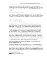
The work required for this analysis is in the le Lemonade.xlsx. (See Figures 17-1, 17-2, and
17-4.) The input assumptions are given in the range D1:D4. I assume that annual demand for
lemonade (see the formula in cell D2) equals 65000–9000*price. (Chapter 79, “Estimating a
Demand Curve,” contains a discussion of how to estimate a demand curve.) I’ve created the
names in C1:C7 to correspond to cells D1:D7.
I computed annual revenue in cell D5 with the formula demand*price. In cell D6, I computed
the annual variable cost with the formula unit cost*demand. Finally, in cell D7, I computed
prot by using the formula revenue–xed cost–variable cost.
FIGURE 17-1 The nputs that change the protab ty of a emonade store.
Suppose that I want to know how changes in price (for example, from $1.00 through $4.00
in $0.25 increments) affect annual prot, revenue, and variable cost. Because I’m changing
only one input, a one-way data table will solve the problem. The data table is shown in
Figure 17-2.
Chapter 17 Sensitivity Analysis with Data Tables 129
FIGURE 17-2 One way data tab e w th vary ng pr ces.
To set up a one-way data table, begin by listing input values in a column. I listed the prices of
interest (ranging from $1.00 through $4.00 in $0.25 increments) in the range C11:C23. Next,
I moved over one column and up one row from the list of input values, and there I listed the
formulas I want the data table to calculate. I entered the formula for prot in cell D10, the
formula for revenue in cell E10, and the formula for variable cost in cell F10.
Now select the table range (C10:F23). The table range begins one row above the rst input;
its last row is the row containing the last input value. The rst column in the table range is

the column containing the inputs; its last column is the last column containing an output.
After selecting the table range, display the Data tab on the ribbon. In the Data Tools group,
click What-If Analysis, and then click Data Table. Now ll in the Data Table dialog box as
shown in Figure 17-3.
FIGURE 17-3 Creat ng a data tab e.
For the column input cell, you use the cell in which you want the listed inputs—that is, the
values listed in the rst column of the data table range—to be assigned. Because the listed
inputs are prices, I chose D1 as the column input cell. After you click OK, Excel creates the
one-way data table shown in Figure 17-4.
130 Microsoft Excel 2010: Data Analysis and Business Modeling
FIGURE 17-4 One way data tab e w th vary ng pr ces.
In the range D11:F11, prot, revenue, and variable cost are computed for a price of $1.00.
In cells D12:F12, prot, revenue, and variable cost are computed for a price of $1.25, and on
through the range of prices. The prot-maximizing price among all listed prices is $3.75. A
price of $3.75 would produce an annual prot of $58,125.00, annual revenue of $117,187.50,
and an annual variable cost of $14,062.50.
Suppose I want to determine how annual prot varies as price varies from $1.50 through
$5.00 (in $0.25 increments) and unit cost varies from $0.30 through $0.60 (in $0.05 incre-
ments). Because here I’m changing two inputs, I need a two-way data table. (See Figure 17-5.)
I list the values for one input down the rst column of the table range (I’m using the range
H11:H25 for the price values) and the values for the other input in the rst row of the table
range. (In this example, the range I10:O10 holds the list of unit cost values.) A two-way data
table can have only one output cell, and the formula for the output must be placed in the
upper-left corner of the table range. Therefore, I placed the prot formula in cell H10.
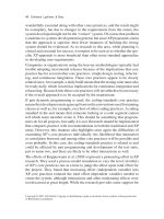
FIGURE 17-5 A two way data tab e show ng prot as a funct on of pr ce and un t var ab e cost.
Chapter 17 Sensitivity Analysis with Data Tables 131
I select the table range (cells H10:O25) and display the Data tab. In the Data Tools group, I
click What-If Analysis and then click Data Table. Cell D1 (price) is the column input cell, and
cell D3 (unit variable cost) is the row input cell. These settings ensure that the values in the
rst column of the table range are used as prices, and the values in the rst row of the table

range are used as unit variable costs. After clicking OK, we see the two-way data table shown
in Figure 17-5. As an example, in cell K19, when we charge $3.50 and the unit variable cost
is $0.40, the annual prot equals $58,850.00. For each unit cost, I’ve highlighted the prot-
maximizing price. Note that as the unit cost increases, the prot-maximizing price increases
as some of the cost increase is passed on to customers. Of course, I can only guarantee that
the prot-maximizing price in the data table is within $0.25 of the actual prot-maximizing
price. When you learn about the Excel Solver in Chapter 79, you’ll learn how to determine (to
the penny) the exact prot-maximizing price.
Here are some other notes on this problem:
■
As you change input values in a worksheet, the values calculated by a data table
change, too. For example, if you increased xed cost by $10,000, all prot numbers in
the data table would be reduced by $10,000.
■
You can’t delete or edit a portion of a data table. If you want to save the values in a
data table, select the table range, copy the values, and then right-click and select Paste
Special. Then choose Values from the Paste Special menu. If you take this step, how-
ever, changes to your worksheet inputs no longer cause the data table calculations to
update.
■
When setting up a two-way data table, be careful not to mix up your row and column
input cells. A mix-up will cause nonsensical results.
■
Most people set their worksheet calculation mode to Automatic. With this setting, any
change in your worksheet will cause all your data tables to be recalculated. Usually,
you want this, but if your data tables are large, automatic recalculation can be in-
credibly slow. If the constant recalculation of data tables is slowing your work down,
click the File tab on the ribbon, click Options, and then click the Formulas tab. Then
select Automatic Except For Data Tables. When Automatic Except For Data Tables is
selected, all your data tables recalculate only when you press the F9 (recalculation) key.

Alternatively, you can click the Calculation Options button (in the Calculation group on
the Formulas tab) and then click Automatic Except For Data Tables.
I am going to build a new house The amount of money I need to borrow (with a 15-year
repayment period) depends on the price for which I sell my current house I’m also unsure
about the annual interest rate I’ll receive when I close Can I determine how my monthly
payments will depend on the amount borrowed and the annual interest rate?
The real power of data tables becomes evident when you combine a data table with one of
the Excel functions. In this example, we’ll use a two-way data table to vary two inputs (the
amount borrowed and the annual interest rate) to the Excel PMT function and determine
132 Microsoft Excel 2010: Data Analysis and Business Modeling
how the monthly payment varies as these inputs change. (The PMT function is discussed in
detail in Chapter 10, “More Excel Financial Functions.”) Our work for this example is in the le
Mortgagedt.xlst, shown in Figure 17-6.
Suppose you’re borrowing money on a 15-year mortgage, where monthly payments are
made at the end of each month. I’ve input the amount borrowed in cell D2, the number of
months in the mortgage (180) in D3, and annual interest rate in D4. I’ve associated the range
names in cells C2:C4 with the cells D2:D4. Based on these inputs, I compute the monthly pay-
ment in D5 with the formula -PMT(Annual int rate/12,Number of Months,Amt Borrowed).
FIGURE 17-6 You can use a data tab e to determ ne how mortgage payments vary as the amount borrowed
and the nterest rate change.
You think that the amount borrowed will range (depending on the price for which you sell
your current house) between $300,000 and $650,000 and that your annual interest rate will
range between 5 percent and 8 percent. In preparation for creating a data table, I entered
the amounts borrowed in the range C8:C15 and possible interest rate values in the range
D7:J7. Cell C7 contains the output you want to recalculate for various input combinations.
Therefore, I set cell C7 equal to cell D5. Next I select the table range (C7:J15), click What-If
Analysis on the Data tab, and then click Data Table. Because numbers in the rst column
of the table range are amounts borrowed, the column input cell is D2. Numbers in the rst
row of the table are annual interest rates, so our row input cell is D4. After you click OK, you
see the data table shown in Figure 17-6. This table shows, for example, that if you borrow

$400,000 at an annual rate of 6 percent, your monthly payments would be just over $3,375.
The data table also shows that at a low interest rate (for example, 5 percent), an increase of
$50,000 in the amount borrowed raises the monthly payment by around $395, whereas at a
high interest rate (such as 8 percent), an increase of $50,000 in the amount borrowed raises
the monthly payment by about $478.
A major Internet company is thinking of purchasing another online retailer The retailer’s
current annual revenues are $100 million, with expenses of $150 million Current
projections indicate that the retailer’s revenues are growing at 25 percent per year and
its expenses are growing at 5 percent per year We know projections might be in error,
however, and we would like to know, for a variety of assumptions about annual revenue
and expense growth, the number of years before the retailer will show a prot
Chapter 17 Sensitivity Analysis with Data Tables 133
We want to determine the number of years needed to break even, using annual growth rates
in revenue from 10 percent through 50 percent and annual expense growth rates from 2
percent through 20 percent. Let’s also assume that if the rm cannot break even in 13 years,
we’ll say “cannot break even.” Our work is in the le Bezos.xlsx, shown in Figures 17-7 and
17-8.
I chose to hide columns A and B and rows 16–18. To hide columns A and B, rst select any
cells in columns A and B (or select the column headings), and then display the Home tab. In
the Cells group, click Format, point to Hide & Unhide, and select Hide Columns. To hide rows
16–18, select any cells in those rows (or select the row headings) and repeat the previous
procedure, selecting Hide Rows. Of course, the Format Visibility options also include Unhide
Rows and Unhide Columns. If you receive a worksheet with many hidden rows and columns
and want to quickly unhide all of them, you can select the entire worksheet by clicking the
Select All button at the intersection of the column and row headings. Now selecting Unhide
Rows and/or Unhide Columns will unhide all hidden rows and/or columns in the worksheet.
In row 11, I project the rm’s revenue out 13 years (based on the annual revenue growth
rate assumed in E7) by copying from F11 to G11:R11 the formula E11*(1+$E$7). In row 12, I
project the rm’s expenses out 13 years (based on the annual expense growth rate assumed
in E8) by copying from F12 to G12:R12 the formula E12*(1+$E$8). (See Figure 17-7.)

FIGURE 17-7 You can use a data tab e to ca cu ate how many years t w take to break even.
We would like to use a two-way data table to determine how varying the growth rates for
revenues and expenses affects the years needed to break even. We need one cell whose
value always tells us the number of years needed to break even. Because we can break even
during any of the next 13 years, this might seem like a tall order.
I begin by using in row 13 an IF statement for each year to determine whether we break even
during the year. The IF statement returns the number of the year if we break even during the
year or 0 otherwise. I determine the year we break even in cell E15 by simply adding together
all the numbers in row 13. Finally, I can use cell E15 as the output cell for a two-way data
table.
I copy from cell F13 to G13:R13 the formula IF(AND(E11<E12,F11>F12),F10,0). This formula
reects the fact that we break even for the rst time during a year if, and only if, during the
previous year, revenues are less than expenses and during the current year, revenues are
greater than expenses. If this is the case, the year number is entered in row 13; otherwise, 0 is
entered.
134 Microsoft Excel 2010: Data Analysis and Business Modeling
Now, in cell E15 I can determine the breakeven year (if any) with the formula
IF(SUM(F13:R13)>0,SUM(F13:R13),”No BE”). If we do not break even during the next 13 years,
the formula enters the text string “No BE”.
I now enter the annual revenue growth rates (10 percent through 50 percent) in the range
E21:E61. I enter annual expense growth rates (2 percent to 20 percent) in the range F20:X20.
I ensure that the year-of-breakeven formula is copied to cell E20 with the formula E15.
Next, I select the table range E20:X61, click What-If Analysis on the Data tab, and then click
Data Table. I select cell E7 (revenue growth rate) as the column input cell and cell E8 (expense
growth rate) as the row input cell. With these settings, I obtain the two-way data table shown
in Figure 17-8.
FIGURE 17-8 A two way data tab e.
Note, for example, that if expenses grow at 4 percent a year, a 10-percent annual growth in
revenue will result in breaking even in eight years, whereas a 50-percent annual growth in
revenue will result in breaking even in only two years! Also note that if expenses grow at 12

percent per year and revenues grow at 14 percent per year, we will not break even by the
end of 13 years.
Problems
1. You’ve been assigned to analyze the protability of Bill Clinton’s autobiography. The
following assumptions have been made:
❑
Bill is receiving a one-time royalty payment of $12 million.
❑
The xed cost of producing the hardcover version of the book is $1 million.
❑
The variable cost of producing each hardcover book is $4.
❑
The publisher’s net from book sales per hardcover unit sold is $15.
❑
The publisher expects to sell 1 million hardcover copies.
❑
The xed cost of producing the paperback is $100,000.
❑
The variable cost of producing each paperback book is $1.
❑
The publisher’s net from book sales per paperback unit sold is $4.
❑
Paperback sales will be double hardcover sales.
Chapter 17 Sensitivity Analysis with Data Tables 135
Use this information to answer the following questions.
❑
Determine how the publisher’s before-tax prot will vary as hardcover sales vary
from 100,000 through 1 million copies.
❑
Determine how the publisher’s before-tax prot varies as hardcover sales vary

from 100,000 through 1 million copies and the ratio of paperback to hardcover
sales varies from 1 through 2.4.
2. The annual demand for a product equals 500-3p+10a
.5
, where p is the price of the
product in dollars and a is hundreds of dollars spent on advertising the product. The
annual xed cost of selling the product is $10,000, and the unit variable cost of pro-
ducing the product is $12. Determine a price (within $10) and amount of advertising
(within $100) that maximizes prot.
3. Reconsider our hedging example from Chapter 12, “IF Statements.” For stock prices
in six months that range from $20 through $65 and the number of puts purchased
varying from 0 through 100 (in increments of 10), determine the percentage return on
your portfolio.
4. For our mortgage example, suppose you know the annual interest rate will be 5.5
percent. Create a table that shows for amounts borrowed from $300,000 through
$600,000 (in $50,000 increments) the difference in payments between a 15-year,
20-year, and 30-year mortgage.
5. Currently, you sell 40,000 units of a product for $45 each. The unit variable cost of
producing the product is $5. You are thinking of cutting the product price by 30
percent. You are sure this will increase sales by an amount from 10 percent through 50
percent. Perform a sensitivity analysis to show how prot will change as a function of
the percentage increase in sales. Ignore xed costs.
6. Let’s assume that at the end of each of the next 40 years, you put the same amount in
your retirement fund and earn the same interest rate each year. Show how the amount
of money you will have at retirement changes as you vary your annual contribution
from $5,000 through $25,000 and the rate of interest varies from 3 percent through
15 percent.
7. The payback period for a project is the number of years needed for a project’s future
prots to pay back the project’s initial investment. A project requires a $300 million
investment at Time 0. The project yields prot for 10 years, and Time 1 cash ow will be

between $30 million and $100 million. Annual cash ow growth will be from 5 percent
through 25 percent a year. How does the project payback depend on the Year 1 cash
ow and cash ow growth rates?
8. A software development company is thinking of translating a software product into
Swahili. Currently, 200,000 units of the product are sold per year at a price of $100
each. Unit variable cost is $20. The xed cost of translation is $5 million. Translating
the product into Swahili will increase sales during each of the next three years by some
136 Microsoft Excel 2010: Data Analysis and Business Modeling
unknown percentage over the current level of 200,000 units. Show how the change in
prot resulting from the translation depends on the percentage increase in product
sales. You can ignore the time value of money and taxes in your calculations.
9. The le Citydistances.xlsx gives latitude and longitude for several U.S. cities. There
is also a formula that determines the distance between two cities by using a given
latitude and longitude. Create a table that computes the distance between any pair of
cities listed.
10. You have begun saving for your child’s college education. You plan to save $5,000 per
year, and want to know for annual rates of return on your investment from 4 percent
through 12 percent the amount of money you will have in the college fund after saving
for 10–15 years.
11. If you earn interest at percentage rate r per year and compound your interest n times
per year, then in y years $1 will grow to (1+(r/n))
ny
dollars. Assuming a 10 percent
annual interest rate, create a table showing the factor by which $1 will grow in 5–15
years for daily, monthly, quarterly, and semiannual compounding.
12. Assume I have $100 in the bank. Each year, I withdraw x percent (ranging from 4
percent through 10 percent) of my original balance. For annual growth rates of 3
percent through 10 percent per year, determine how many years it will take before I
run out of money. Hint: You should use the IFERROR function (discussed in Chapter 12)
because if my annual growth rate exceeds the withdrawal rate, I will never run out of

money.
13. If you earn interest at an annual rate of x percent per year, then in n years $1 will
become (1+x)
n
dollars. For annual rates of interest from 1 percent through 20 percent,
determine the exact time (in years) in which $1 will double.
14. You are borrowing $200,000 and making payments at the end of each month. For an
annual interest rate ranging from 5 percent through 10 percent and loan durations of
10, 15, 20, 25, and 30 years, determine the total interest paid on the loan.
15. You are saving for your child’s college fund. You are going to contribute the same
amount of money to the fund at the end of each year. Your goal is to end up with
$100,000. For annual investment returns ranging from 4 percent through 15 percent
and number of years investing varying from 5–15 years, determine your required
annual contribution.
16. The le Antitrustdata.xlsx gives the starting and ending years for many court cases.
Determine the number of court cases active during each year.
17. You can retire at age 62 and receive $8,000 per year or retire at age 65 and receive
$10,000 per year. What is the difference (in today’s dollars) between these two choices
as you vary the annual rate at which you discount cash ows between 2 percent and 10
percent and vary age of death between 70 and 84?
137
Chapter 18
The Goal Seek Command
Questions answered in this chapter:
■
For a given price, how many glasses of lemonade does a lemonade store need to sell
per year to break even?
■
We want to pay off our mortgage in 15 years. The annual interest rate is 6 percent. The
bank told us we can afford monthly payments of $2,000. How much can we borrow?

■
I always had trouble with “story problems” in high school algebra. Can Excel make
solving story problems easier?
The Goal Seek feature in Microsoft Excel 2010 enables you to compute a value for a
worksheet input that makes the value of a given formula match the goal you specify. For
example, in the lemonade store example in Chapter 17, “Sensitivity Analysis with Data Tables,”
suppose you have xed overhead costs, xed per-unit costs, and a xed sales price. Given
this information, you can use Goal Seek to calculate the number of glasses of lemonade you
need to sell to break even. Essentially, Goal Seek embeds a powerful equation solver in your
worksheet. To use Goal Seek, you need to provide Excel with three pieces of information:
■
Set Cell Species that the cell contains the formula that calculates the information
you’re seeking. In the lemonade example, the Set Cell would contain the formula for
prot.
■
To Value Species the numerical value for the goal that’s calculated in the Set Cell. In
the lemonade example, because we want to determine the sales volume that represents
the breakeven point, the To Value would be 0.
■
By Changing Cell Species the input cell that Excel changes until the Set Cell
calculates the goal dened in the To Value cell. In the lemonade example, the By
Changing Cell would contain annual lemonade sales.
Answers to This Chapter’s Questions
For a given price, how many glasses of lemonade does a lemonade store need to sell per
year to break even?
The work for this section is in the le Lemonadegs.xlsx, which is shown in Figure 18-1. As in
Chapter 17, I’ve assumed an annual xed cost of $45,000.00 and a variable unit cost of $0.45.
Let’s assume a price of $3.00. The question is how many glasses of lemonade do I need to sell
each year to break even.
138 Microsoft Excel 2010: Data Analysis and Business Modeling

FIGURE 18-1 We use th s data to set up the Goa Seek feature to perform a breakeven ana ys s.
To start, insert any number for demand in cell D2. In the What-If Analysis group on the Data
tab, click Goal Seek. Now ll in the Goal Seek dialog box as shown in Figure 18-2.
FIGURE 18-2 The Goa Seek d a og box  ed n w th entr es for a breakeven ana ys s.
The dialog box indicates that I want to change cell D2 (annual demand, or sales) until cell D7
(prot) hits a value of 0. After I click OK, I get the result that’s shown in Figure 18-1. If I sell
approximately 17,647 glasses of lemonade per year (or 48 glasses per day), I’ll break even. To
nd the value I’m seeking, Excel varies the demand in cell D2 (alternating between high and
low values) until it nds a value that makes prot equal $0. If a problem has more than one
solution, Goal Seek will still display only one answer.
We want to pay off our mortgage in 15 years The annual interest rate is 6 percent The
bank told us we can afford monthly payments of $2,000 How much can we borrow?
You can begin to answer this question by setting up a worksheet to compute the monthly
payments on a 15-year loan (let’s assume payments at the end of the month) as a function
of the annual interest rate and a trial loan amount. You can see the work I did in the le
Paymentgs.xlsx and in Figure 18-3.
In cell E6, the formula –PMT(annual int rate/12,years,amt. borrowed) computes the monthly
payment associated with the amount borrowed, which is listed in cell E5. Filling in the Goal
Seek dialog box as shown in Figure 18-4 calculates the amount borrowed that results in
monthly payments equal to $2,000. With a limit of $2,000 for monthly payments, you can
borrow up to $237,007.03.
Chapter 18 The Goal Seek Command 139
FIGURE 18-3 You can use data such as th s w th the Goa Seek feature to determ ne the amount you can
borrow based on a set month y payment.
FIGURE 18-4 The Goa Seek d a og box set up to ca cu ate the mortgage examp e.
I always had trouble with “story problems” in high school algebra Can Excel make solving
story problems easier?
If you think back to high school algebra, most story problems required you to choose a
variable (usually it was called x) that solved a particular equation. Goal Seek is an equation
solver, so it’s perfectly suited to solving story problems. Here’s a typical high school algebra

problem:
Maria and Edmund have a lover’s quarrel while honeymooning in Seattle. Maria storms into
her Mazda Miata and drives 64 miles per hour toward her mother’s home in Los Angeles. Two
hours after Maria leaves, Edmund jumps into his BMW in hot pursuit, driving 80 miles per
hour. How many miles will each person have traveled when Edmund catches Maria?
You can nd the solution in the le Maria.xlsx, shown in Figure 18-5.
FIGURE 18-5 Goa Seek can he p you so ve story prob ems.
The Set Cell will be the difference between the distances Maria and Edmund have traveled.
You can set this to a value of 0 by changing the number of hours Maria drives. Of course,
Edmund drives two hours less than Maria.
140 Microsoft Excel 2010: Data Analysis and Business Modeling
I entered a trial number of hours that Maria drives in cell D2. Then I associated the range
names in the cell range C2:C8 with cells D2:D8. Because Edmund drives two fewer hours than
Maria, in cell D4 I entered the formula Time Maria drives–2. In cells D6 and D7, I used the
fact that distance speed*time to compute the total distance Maria and Edmund travel. The
difference between the distances traveled by Edmund and Maria is computed in cell D8 with
the formula Maria distance–Edmund distance. Now I can ll in the Goal Seek dialog box as
shown in Figure 18-6.
FIGURE 18-6 The Goa Seek d a og box  ed n to so ve an a gebra story prob em.
I change Maria’s hours of driving (cell D2) until the difference between the miles traveled
by Edmund and Maria (cell D8) equals 0. As you can see, after Maria drives 10 hours and
Edmund 8 hours, they will each have driven a distance of 640 miles.
Problems
1. From Problem 1 in Chapter 17, determine how many hardcover books must be sold to
break even.
2. From the car net present value (NPV) example in Chapter 16, “The Auditing Tool,” by
what rate do annual sales need to grow for total NPV to equal $1 million?
3. What value of Year 1 unit cost would increase our NPV in the car example in Chapter 16
to $1 million?
4. In our mortgage example, suppose I need to borrow $200,000 for 15 years. If my

maximum payments are limited to $2,000 per month, how high an annual interest rate
can I tolerate?
5. How could I use Goal Seek to determine a project’s internal rate of return (IRR)?
6. At the end of each of the next 40 years, I’m going to put $20,000 in my retirement
fund. What rate of return on my investments do I need so that I will have $2 million
available for retirement in 40 years?
7. I expect to earn 10 percent per year on my retirement investments. At the end of each
of the next 40 years, I want to put the same amount of money in my retirement port-
folio. How much money do I need to put in each year if I want to have $2 million in my
account when I retire?
Chapter 18 The Goal Seek Command 141
8. Consider two projects with the following cash ows:
Year 1 Year 2 Year 3 Year 4
Project 1 –$1,000 $400 $350 $400
Project 2 –$900 $100 $100 $1,000
For what rate of interest will Project 1 have a larger NPV? (Hint: Find the interest rate
that makes both projects have the same NPV.)
9. I am managing a conference at my college. My xed costs are $15,000. I must pay the
10 speakers $700 each, and the college union $300 per conference participant for food
and lodging costs. I am charging each conference participant who is not also a speaker
$900, which includes the conference fee and their food and lodging costs. How many
paid registrants need to attend for me to break even?
10. I am buying 40 pounds of candy. Some of the candy sells for $10 per pound and some
sells for $6 per pound. How much candy at each price should I buy to result in an
average cost of $7 per pound?
11. Three electricians are wiring my new home. Electrician 1 by himself will need 11 days to
do the job. Electrician 2 by himself will need 5 days to do the job. Electrician 3 by her-
self will need 9 days to do the job. If all three electricians work on the job, how long will
the job take to complete?
12. To celebrate the Lewis and Clark Expedition, I am traveling 40 miles upstream and then

40 miles downstream in a canoe. The speed of the river current is 5 miles per hour. If
the trip takes me 5 hours total, how fast do I travel if the river has no current?
13. In the NPV.xlsx le in Chapter 8, “Evaluating Investments by Using Net Present Value
Criteria,” we found that for high interest rates Project 1 has a larger NPV and for small
interest rates Project 2 has a larger NPV. For what interest rate would the two projects
have the same NPV?
143
Chapter 19
Using the Scenario Manager for
Sensitivity Analysis
Question answered in this chapter:
■
I’d like to create best, worst, and most-likely scenarios for the sales of an automobile
by varying the values of Year 1 sales, annual sales growth, and Year 1 sales price. Data
tables for sensitivity analysis allow me to vary only one or two inputs, so I can’t use a
data table. Does Excel have a tool I can use to vary more than two inputs in a sensitivity
analysis?
You can use the Scenario Manager to perform sensitivity analysis by varying as many as 32
input cells. With the Scenario Manager, you rst dene the set of input cells you want to
vary. Next, you name your scenario and enter for each scenario the value of each input cell.
Finally, you select the output cells (also called result cells) that you want to track. The Scenario
Manager then creates a beautiful report containing the inputs and the values of the output
cells for each scenario.
Answer to This Chapter’s Question
I’d like to create best, worst, and most-likely scenarios for the sales of an automobile by
varying the values of Year 1 sales, annual sales growth, and Year 1 sales price Data tables
for sensitivity analysis allow me to vary only one or two inputs, so I can’t use a data table
Does Excel have a tool I can use to vary more than two inputs in a sensitivity analysis?
Suppose you want to create the following three scenarios related to the net present value
(NPV) of a car, using the example in Chapter 16, “The Auditing Tool.”

Year 1 sales Annual sales growth Year 1 sales price
Best case $20,000 20% $10 00
Most ke y case $10,000 10% $7 50
Worst case $5,000 2% $5 00
For each scenario, you want to look at the rm’s NPV and each year’s after-tax prot. The
work is in the le NPVauditscenario.xlsx. Figure 19-1 shows the worksheet model (contained
in the Original Model worksheet), and Figure 19-2 shows the scenario report (contained in
the Scenario Summary worksheet).
144 Microsoft Excel 2010: Data Analysis and Business Modeling
FIGURE 19-1 The data on wh ch the scenar os are based.
FIGURE 19-2 The scenar o summary report.
To begin dening the best-case scenario, display the Data tab, and then click Scenario
Manager on the What-If Analysis menu in the Data Tools group. Then click the Add button,
and ll in the Add Scenario dialog box as shown in Figure 19-3.
Chapter 19 Using the Scenario Manager for Sensitivity Analysis 145
FIGURE 19-3 Data nputs for the best case scenar o.
Enter a name for the scenario (Best), and select C2:C4 as the input cells containing the values
that dene the scenario. After you click OK in the Add Scenario dialog box, ll in the Scenario
Values dialog box with the input values that dene the best case, as shown in Figure 19-4.
FIGURE 19-4 Den ng the nput va ues for the best case scenar o.
By clicking Add in the Scenario Values dialog box, you can enter the data for the most-likely
and worst-case scenarios. After entering data for all three scenarios, click OK in the Scenario
Values dialog box. The Scenario Manager dialog box, shown in Figure 19-5, lists the scenarios
I created. When you click Summary in the Scenario Manager dialog box, you can choose the
result cells that will be displayed in scenario reports. Figure 19-6 shows how I indicated in the
Scenario Summary dialog box that I want the scenario summary report to track each year’s
after-tax prot (cells B17:F17) as well as total NPV (cell B19).
146 Microsoft Excel 2010: Data Analysis and Business Modeling
FIGURE 19-5 The Scenar o Manager d a og box d sp ays each scenar o you dene.
FIGURE 19-6 Use the Scenar o Summary d a og box to se ect the resu t ce s for the summary report.

Because the result cells come from more than one range, I separated the ranges B17:F17 and
B19 with a comma. (I could also have used the Ctrl key to select and enter multiple ranges.)
After selecting Scenario Summary (instead of the PivotTable option), click OK, and Excel cre-
ates the beautiful Scenario Summary report pictured earlier in Figure 19-2. Notice that Excel
includes a column, labeled Current Values, for the values that were originally placed in the
worksheet. The worst case loses money (a loss of $13,345.75), whereas the best case is quite
protable (a prot of $226,892.67). Because the worst-case price is less than our variable cost,
the worst case loses money in each year.
Remarks
■
The Scenario PivotTable Report option on the Scenario Summary dialog box presents
the scenario results in a PivotTable format.
■
Suppose you select a scenario in the Scenario Manager dialog box and then click the
Show button. The input cells’ values for the selected scenario then appear in the work-
sheet, and Excel recalculates all formulas. This tool is great for presenting a “slide show”
of your scenarios.
Chapter 19 Using the Scenario Manager for Sensitivity Analysis 147
■
It’s hard to create a lot of scenarios with the Scenario Manager because you need
to input each individual scenario’s values. Monte Carlo simulation (see Chapter 69,
“Introduction to Monte Carlo Simulation”) makes it easy to create many scenarios.
Using the Monte Carlo simulation method, you can nd information such as the
probability that the NPV of a project’s cash ows is nonnegative—an important mea-
sure because it is the probability that the project adds value to the company.
■
Clicking the minus (–) sign in row 5 of the Scenario Summary report hides the
Assumption cells and show only results. Clicking the plus (+) sign restores the full
report.
■

Suppose you send a le to several people, and each adds his or her own scenarios.
After each person returns the le containing the scenarios to you, you can merge all
the scenarios into one workbook by opening each person’s version of the workbook,
clicking the Merge button in the Scenario Manager dialog box in the original work-
book, and then selecting the workbooks containing the scenarios you want to merge.
Excel merges the selected scenarios in the original workbook.
Problems
1. Delete the best-case scenario and run another scenario report.
2. Add a scenario named High Price, in which Year 1 price equals $15 and the other two
inputs remain at their most-likely values.
3. For the lemonade stand example in Chapter 17, “Sensitivity Analysis with Data Tables,”
use the Scenario Manager to display a report summarizing prot for the following
scenarios:
Scenario Price Unit cost Fixed cost
H gh cost/h gh pr ce $5 00 $1 00 $65,000 00
Med um cost/med um pr ce $4 00 $0 75 $45,000 00
Low cost/ ow pr ce $2 50 $0 40 $25,000 00

4. For the mortgage payment example in Chapter 17, use the Scenario Manager to create
a report tabulating monthly payments for the following scenarios:
Scenario Amount borrowed Annual rate Number of monthly
payments
Lowest payment $300,000 4% 360
Most- ke y payment $400,000 6% 240
H ghest payment $550,000 8% 180
149
Chapter 20
The COUNTIF, COUNTIFS, COUNT,
COUNTA, and COUNTBLANK
Functions

Questions answered in this chapter:
■
Suppose I have a list of songs that were played on the radio. For each song, I know the
singer, the date the song was played, and the length of the song. How can I answer
questions such as these about the songs in the list:
❑
How many were sung by each singer?
❑
How many were not sung by my favorite singer?
❑
How many were at least four minutes long?
❑
How many were longer than the average length of all songs on the list?
❑
How many were sung by singers whose last names begin with S?
❑
How many were sung by singers whose last names contain exactly six letters?
❑
How many were played after June 15, 2005?
❑
How many were played before 2009?
❑
How many were exactly four minutes long?
❑
How many were sung by my favorite singer and were exactly four minutes long?
❑
How many were sung by my favorite singer and were three to four minutes long?
In a more general context, how do I perform operations such as the following:
■
Count the number of cells in a range containing numbers.

■
Count the number of blank cells in a range.
■
Count the number of nonblank cells in a range.
You often need to count the number of cells in a range that meet a given criterion. For
example, if a worksheet contains information about makeup sales, you might want to count
the number of sales transactions made by the salesperson named Jennifer or the number of
sales transactions that occurred after June 10. The COUNTIF function lets you count the num-
ber of cells in a range that meet criteria that are dened on the basis of a one row or column
of the worksheet.
150 Microsoft Excel 2010: Data Analysis and Business Modeling
The syntax of the COUNTIF function is COUNTIF(range,criterion).
■
Range is the range of cells in which you want to count cells meeting a given criterion.
■
Criterion is a number, date, or expression that determines whether to count a given cell
in the range.
The syntax of COUNTIFS is COUNTIFS(range1,criterion1,range2,criterion2,…,range n,criterion n).
COUNTIFS counts the number of rows for which the range1 entry meets criterion1, the
range2 entry meets criterion2, the range n entry meets criterion n, and so on. Thus,
COUNTIFS allows the criteria to involve more than one column or multiple conditions in one
column. Other functions that allow for multiple criteria are discussed in Chapter 21, “The
SUMIF, AVERAGEIF, SUMIFS, and AVERAGEIFS Functions,” and Chapter 45, “Summarizing Data
with Database Statistical Functions.”
The key to using the COUNTIF function (and similar functions) successfully is understanding
the wide variety of criteria that Excel accepts. The types of criteria you can use are best
explained through the use of examples. In addition to examples of the COUNTIF function, I’ll
provide examples of the COUNT, COUNTA, and COUNTBLANK functions:
■
The COUNT function counts the number of cells in a range containing numbers.

■
The COUNTA function counts the number of nonblank cells in a range.
■
The COUNTBLANK function counts the number of blank cells in a range.
As an illustration of how to use these functions, consider a database that gives the following
information for each song played on radio station WKRP:
■
The singer
■
The date the song was played
■
The length of the song
The le Rock.xlsx, shown in Figure 20-1, shows a subset of the data.
Chapter 20 The COUNTIF, COUNTIFS, COUNT, COUNTA, and COUNTBLANK Functions 151
FIGURE 20-1 The song database used for the COUNT F examp es.
Answers to This Chapter’s Questions
How many songs were sung by each singer?
To begin, I selected the rst row of the database, the range D6:G6. Then I selected the
whole database by pressing Ctrl+Shift+Down Arrow. Next, in the Dened Names group on
the Formulas tab, I clicked Create From Selection and then chose Top Row. This names the
range D7:D957 Song Numb, the range E7:E957 Singer, the range F7:F957 Date, and the range
G7:G957 Minutes. To determine how many songs were sung by each singer, you copy from
C5 to C6:C12 the formula COUNTIF(Singer,B5). In cell C5, this formula now displays the num-
ber of cells in the range Singer that match the value in B5 (Eminem). The database contains
114 songs sung by Eminem. Similarly, Cher sang 112 songs, and so on, as you can see in
Figure 20-2. I could have also found the number of songs sung by Eminem with the formula
COUNTIF(Singer,”Eminem”). Note that you must enclose text such as Eminem in quotation
marks (“ “) and that criteria are not case sensitive.
FIGURE 20-2 Us ng COUNT F to determ ne how many songs were sung by each s nger.
152 Microsoft Excel 2010: Data Analysis and Business Modeling

How many songs were not sung by Eminem?
To solve this problem, you need to know that Excel interprets the character combination <>
as “not equal to.” The formula COUNTIF(Singer,”<>Eminem”), entered in cell C15, tells you
that 837 songs in the database were not sung by Eminem, as you can see in Figure 20-3. I
need to enclose <>Eminem in quotation marks because Excel treats the not equal to (<>)
character combination as text and Eminem is, of course, text. You could obtain the same
r esult by using the formula COUNTIF(Singer,”<>”&B5), which uses the ampersand (&) symbol
to concatenate the reference to cell B5 and the <> operator.
FIGURE 20-3 You can comb ne the COUNT F funct on w th the not equa to operator (<>).
How many songs were at least four minutes long?
In cell C16, I computed the number of songs played that lasted at least four minutes by using
the formula COUNTIF(Minutes,”> 4”). You need to enclose > 4 in quotation marks because
the greater than or equal to (> ) character combination, like <>, is treated as text. You can
see that 477 songs lasted at least four minutes.
How many songs were longer than the average length of all songs on the list?
To answer this question, I rst computed in cell G5 the average length of a song with the
formula AVERAGE(Minutes). Then, in cell C17, I computed the number of songs that last
longer than the average with the formula COUNTIF(Minutes,”>”&G5). I can refer to another
cell (in this case G5) in the criteria by using the & character. You can see that 477 songs lasted
longer than average, which matches the number of songs lasting at least 4 minutes. The
reason these numbers match is that I assumed the length of each song was an integer. For a
song to last at least 3.48 minutes, it has to last at least 4 minutes.
How many songs were sung by singers whose last names begin with S?
To answer this question, I used a wildcard character, the asterisk (*), in the criteria. An asterisk
represents any sequence of characters. Thus, the formula COUNTIF(Singer,”S*”) in cell C18
picks up any song sung by a singer whose last name begins with S. (The criteria are not case
sensitive.) Two hundred thirty-two songs were sung by singers with last names that begin
with S. This number is simply the total of the songs sung by Bruce Springsteen and Britney
Spears (103+129 232).
Chapter 20 The COUNTIF, COUNTIFS, COUNT, COUNTA, and COUNTBLANK Functions 153

How many songs were sung by singers whose last names contain exactly six letters?
In this example, I used the question mark (?) wildcard character. The question mark matches
any character. Therefore, entering the formula COUNTIF(Singer,”??????”) in cell C19 counts
the number of songs sung by singers having six letters in their last name. The result is 243.
(Two singers have last names of six characters, Britney Spears and Eminem, who together
sang a total of 243 songs—129+114 243.)
How many songs were played after June 15, 2005?
The criteria you use with COUNTIF functions handle dates on the basis of a date’s
serial number. (A later date is considered larger than an earlier date.) The formula
COUNTIF(Date,”>6/15/2005”) in cell C20 tells you that 98 songs were played after
June 15, 2005.
How many songs were played before 2009?
Here, we want our criteria to pick up all dates on or before December 31, 2008. I entered
in cell C21 the formula COUNTIF(Date,”< 12/31/2008”). You can see that 951 songs (which
turns out to be all the songs) were played before the start of 2009.
How many songs were exactly four minutes long?
In cell C22, I computed the number of songs lasting exactly four minutes with the formula
COUNTIF(Minutes,4). This formula counts the number of cells in the range G7:G957 contain-
ing a 4. As you can see, 247 songs lasted exactly four minutes. In a similar fashion, cell C23
shows that 230 songs lasted exactly ve minutes.
How many songs played were sung by Bruce Springsteen and were exactly four minutes
long?
We want to count each row where an entry in the Singer column is Springsteen and an
entry in the Minutes column is 4. Since this question involves more than one criteria, this
is a job for the wonderful COUNTIFS function. Simply enter in cell C24 the formula
COUNTIFS(Singer,”Springsteen”,Minutes,4).
This formula counts any row in which Singer is Springsteen and Minutes equals 4. Bruce
Springsteen sang 24 songs that were exactly four minutes long. My favorite Springsteen song
is “Thunder Road,” but that song is more than four minutes long. I recommend using the
function wizard to input formulas involving the COUNTIFS function. Don’t forget that you

can paste range names into your formula with the F3 key.
How many songs played were sung by Madonna and were three to four minutes long?
Because we are dealing with multiple criteria, this is again a job for COUNTIFS. Entering in cell
C25 the formula COUNTIFS(Singer,”Madonna”,Minutes,”< 4”,Minutes,”> 3”) counts all rows
in which Madonna sang a song that was from three to four minutes long. These are exactly
154 Microsoft Excel 2010: Data Analysis and Business Modeling
the rows we want to count. It turns out that Madonna sang 70 songs that were from three to
four minutes long. (My favorite one is “Crazy for You!”)
How do I count the number of cells in a range containing numbers?
The COUNT function counts the number of cells in a range containing a numeric value. For
example, the formula COUNT(B5:C14) in cell C2 displays 9 because nine cells (the cells in
C5:C13) in the range B5:C14 contain numbers. (See Figure 20-2.)
How do I count the number of blank cells in a range?
The COUNTBLANK function counts the number of blank cells in a range. For example, the
formula COUNTBLANK(B5:C14) entered in cell C4 returns a value of 2 because two cells (B14
and C14) in the range B5:C14 contain blanks.
How do I count the number of nonblank cells in a range?
The COUNTA function returns the number of nonblank cells in a range. For example, the
formula COUNTA(B5:C14) in cell C3 returns 18 because 18 cells in the range B5:C14 are not
blank.
Remarks
In the remainder of the book I discuss alternative methods to answer questions involving two
or more criteria (such as how many Britney Spears songs were played before June 10, 2005).
■
Database statistical functions are discussed in Chapter 45, “Summarizing Data with
Database Statistical Functions.”
■
Array formulas are discussed in Chapter 83, “Array Formulas and Functions.”
Problems
The following questions refer to the le Rock.xlsx.

1. How many songs were not sung by Britney Spears?
2. How many songs were played before June 15, 2004?
3. How many songs were played between June 1, 2004, and July 4, 2006? Hint: Take the
difference between two COUNTIF functions.
4. How many songs were sung by singers whose last names begin with M?
5. How many songs were sung by singers whose names contain an e?
6. Create a formula that always yields the number of songs played today. Hint: Use the
TODAY() function.