Báo cáo y học: "Statistics review 14: Logistic regression" doc
Bạn đang xem bản rút gọn của tài liệu. Xem và tải ngay bản đầy đủ của tài liệu tại đây (114.26 KB, 7 trang )
112
AUROC = area under the receiver operating characteristic curve; C.I. = confidence interval; ln = natural logarithm; logit = natural logarithm of the
odds; MLE = maximum likelihood estimate; OR = odds ratio; ROC = receiver operating characteristic curve.
Critical Care February 2005 Vol 9 No 1 Bewick et al.
Introduction
Logistic regression provides a method for modelling a binary
response variable, which takes values 1 and 0. For example,
we may wish to investigate how death (1) or survival (0) of
patients can be predicted by the level of one or more
metabolic markers. As an illustrative example, consider a
sample of 2000 patients whose levels of a metabolic marker
have been measured. Table 1 shows the data grouped into
categories according to metabolic marker level, and the
proportion of deaths in each category is given. The
proportions of deaths are estimates of the probabilities of
death in each category. Figure 1 shows a plot of these
proportions. It suggests that the probability of death
increases with the metabolic marker level. However, it can
be seen that the relationship is nonlinear and that the
probability of death changes very little at the high or low
extremes of marker level. This pattern is typical because
proportions cannot lie outside the range from 0 to 1. The
relationship can be described as following an ‘S’-shaped
curve.
Logistic regression with a single quantitative
explanatory variable
The logistic or logit function is used to transform an ‘S’-
shaped curve into an approximately straight line and to
change the range of the proportion from 0–1 to –∞ to +∞.
The logit function is defined as the natural logarithm (ln) of
the odds [1] of death. That is,
p
logit(p) = ln
( )
1 – p
Where p is the probability of death.
Figure 2 shows the logit-transformed proportions from Fig. 1.
The points now follow an approximately straight line. The
relationship between probability of death and marker level x
could therefore be modelled as follows:
logit(p) = a + bx
Although this model looks similar to a simple linear regression
model, the underlying distribution is binomial and the
parameters a and b cannot be estimated in exactly the same
way as for simple linear regression. Instead, the parameters
are usually estimated using the method of maximum
likelihood, which is discussed below.
Binomial distribution
When the response variable is binary (e.g. death or survival),
then the probability distribution of the number of deaths in a
sample of a particular size, for given values of the explanatory
Review
Statistics review 14: Logistic regression
Viv Bewick
1
, Liz Cheek
1
and Jonathan Ball
2
1
Senior Lecturer, School of Computing, Mathematical and Information Sciences, University of Brighton, Brighton, UK
2
Senior Registrar in ICU, Liverpool Hospital, Sydney, Australia
Corresponding author: Viv Bewick,
Published online: 13 January 2005 Critical Care 2005, 9:112-118 (DOI 10.1186/cc3045)
This article is online at />© 2005 BioMed Central Ltd
Abstract
This review introduces logistic regression, which is a method for modelling the dependence of a binary
response variable on one or more explanatory variables. Continuous and categorical explanatory
variables are considered.
Keywords binomial distribution, Hosmer–Lemeshow test, likelihood, likelihood ratio test, logit function, maximum
likelihood estimation, median effective level, odds, odds ratio, predicted probability, Wald test
113
Available online />variables, is usually assumed to be binomial. The probability
that the number of deaths in a sample of size n is exactly
equal to a value r is given by
n
C
r
p
r
(1 – p)
n – r
, where
n
C
r
=
n!/(r!(n – r)!) is the number of ways r individuals can be
chosen from n and p is the probability of an individual dying.
(The probability of survival is 1 – p.)
For example, using the first row of the data in Table 1, the
probability that seven deaths occurred out of 182 patients is
given by
182
C
7
p
7
(1 – p)
175
. If the probability of death is
assumed to be 0.04, then the probability that seven deaths
occurred is
182
C
7
× 0.04
7
× 0.86
175
= 0.152. This
probability, calculated on the assumption of a binomial
distribution with parameter p = 0.04, is called a likelihood.
Maximum likelihood estimation
Maximum likelihood estimation involves finding the value(s) of
the parameter(s) that give rise to the maximum likelihood. For
example, again we shall take the seven deaths occurring out
of 182 patients and use maximum likelihood estimation to
estimate the probability of death, p. Figure 3 shows the
likelihood calculated for a range of values of p. From the
graph it can be seen that the value of p giving the maximum
likelihood is close to 0.04. This value is the maximum
likelihood estimate (MLE) of p. Mathematically, it can be
shown that the MLE in this case is 7/182.
In more complicated situations, iterative techniques are
required to find the maximum likelihood and the associated
parameter values, and a computer package is required.
Odds
The model logit(p) = a + bx is equivalent to the following:
p
= odds of death = e
(a + bx)
= e
a
e
bx
1 – p
e
(a + bx)
or p = probability of death =
1 + e
(a + bx)
Because the explanatory variable x increases by one unit from x
to x + 1, the odds of death change from e
a
e
bx
to e
a
e
b(x + 1)
=
e
a
e
bx
e
b
. The odds ratio (OR) is therefore e
a
e
bx
e
b
/e
a
e
bx
= e
b
. The
odds ratio e
b
has a simpler interpretation in the case of a
categorical explanatory variable with two categories; in this case
it is just the odds ratio for one category compared with the other.
Estimates of the parameters a and b are usually obtained
using a statistical package, and the output for the data
Figure 1
Proportion of deaths plotted against the metabolic marker group mid-
points for the data presented in Table 1.
Figure 2
Logit(p) plotted against the metabolic marker group mid-points for the
data presented in Table 1.
Table 1
Relationship between level of a metabolic marker and survival
Metabolic Number of Number of Proportion of
marker level (x) patients deaths deaths
0.5 to <1.0 182 7 0.04
1.0 to <1.5 233 27 0.12
1.5 to <2.0 224 44 0.20
2.0 to <2.5 236 91 0.39
2.5 to <3.0 225 130 0.58
3.0 to <3.5 215 168 0.78
3.5 to <4.0 221 194 0.88
4.0 to <4.5 200 191 0.96
≥4.5 264 260 0.98
Totals 2000 1112
114
Critical Care February 2005 Vol 9 No 1 Bewick et al.
summarized in Table 1 is given in Table 2. From the output,
b = 1.690 and e
b
OR = 5.4. This indicates that, for example,
the odds of death for a patient with a marker level of 3.0 is
5.4 times that of a patient with marker level 2.0.
Predicted probabilities
The model can be used to calculate the predicted probability
of death (p) for a given value of the metabolic marker. For
example, patients with metabolic marker level 2.0 and 3.0
have the following respective predicted probabilities of death:
e
(–4.229 + 1.690 × 2.0)
p = = 0.300
1 + e
(–4.229 + 1.690 × 2.0)
and
e
(–4.229 + 1.690 × 3.0)
p = = 0.700
1 + e
(–4.229 + 1.690 × 3.0)
The corresponding odds of death for these patients are
0.300/(1 – 0.300) = 0.428 and 0.700/(1 – 0.700) = 2.320,
giving an odds ratio of 2.320/0.428 = 5.421, as above.
The metabolic marker level at which the predicted probability
equals 0.5 – that is, at which the two possible outcomes are
equally likely – is called the median effective level (EL
50
).
Solving the equation
e
(a + bx)
p = 0.5 =
1 + e
(a + bx)
gives x = EL
50
= a/b
For the example data, EL
50
= 4.229/1.690 = 2.50, indicating
that at this marker level death or survival are equally likely.
Assessment of the fitted model
After estimating the coefficients, there are several steps
involved in assessing the appropriateness, adequacy and
usefulness of the model. First, the importance of each of the
explanatory variables is assessed by carrying out statistical
tests of the significance of the coefficients. The overall
goodness of fit of the model is then tested. Additionally, the
ability of the model to discriminate between the two groups
defined by the response variable is evaluated. Finally, if
possible, the model is validated by checking the goodness of
fit and discrimination on a different set of data from that which
was used to develop the model.
Tests and confidence intervals for the parameters
The Wald statistic
Wald χ
2
statistics are used to test the significance of individual
coefficients in the model and are calculated as follows:
coefficient
2
()
SE coefficient
Each Wald statistic is compared with a χ
2
distribution with 1
degree of freedom. Wald statistics are easy to calculate but
their reliability is questionable, particularly for small samples.
For data that produce large estimates of the coefficient, the
standard error is often inflated, resulting in a lower Wald
statistic, and therefore the explanatory variable may be
incorrectly assumed to be unimportant in the model. Likelihood
ratio tests (see below) are generally considered to be superior.
The Wald tests for the example data are given in Table 2. The
test for the coefficient of the metabolic marker indicates that the
metabolic marker contributes significantly in predicting death.
Figure 3
Likelihood for a range of values of p. MLE, maximum likelihood estimate.
Table 2
Output from a statistical package for logistic regression on the example data
95% CI for OR
Coefficient SE Wald df P OR Lower Upper
Marker 1.690 0.071 571.074 1 0.000 5.421 4.719 6.227
Constant –4.229 0.191 489.556 1 0.000
CI, confidence interval; df, degrees of freedom; OR, odds ratio; SE, standard error.
115
The constant has no simple practical interpretation but is
generally retained in the model irrespective of its significance.
Likelihood ratio test
The likelihood ratio test for a particular parameter compares
the likelihood of obtaining the data when the parameter is
zero (L
0
) with the likelihood (L
1
) of obtaining the data
evaluated at the MLE of the parameter. The test statistic is
calculated as follows:
–2 × ln(likelihood ratio) = –2 × ln(L
0
/L
1
) = –2 × (lnL
0
– lnL
1
)
It is compared with a χ
2
distribution with 1 degree of
freedom. Table 3 shows the likelihood ratio test for the
example data obtained from a statistical package and again
indicates that the metabolic marker contributes significantly in
predicting death.
Goodness of fit of the model
The goodness of fit or calibration of a model measures how
well the model describes the response variable. Assessing
goodness of fit involves investigating how close values
predicted by the model are to the observed values.
When there is only one explanatory variable, as for the
example data, it is possible to examine the goodness of fit of
the model by grouping the explanatory variable into
categories and comparing the observed and expected counts
in the categories. For example, for each of the 182 patients
with metabolic marker level less than one the predicted
probability of death was calculated using the formula
e
(–4.229 + 1.690 × x)
1 + e
(–4.229 + 1.690 × x)
where x is the metabolic marker level for an individual patient.
This gives 182 predicted probabilities from which the
arithmetic mean was calculated, giving a value of 0.04. This
was repeated for all metabolic marker level categories.
Table 4 shows the predicted probabilities of death in each
category and also the expected number of deaths calculated
as the predicted probability multiplied by the number of
patients in the category. The observed and the expected
numbers of deaths can be compared using a χ
2
goodness of
fit test, providing the expected number in any category is not
less than 5. The null hypothesis for the test is that the
numbers of deaths follow the logistic regression model. The
χ
2
test statistic is given by
(observed – expected)
2
χ
2
=
Σ
expected
The test statistic is compared with a χ
2
distribution where the
degrees of freedom are equal to the number of categories
minus the number of parameters in the logistic regression
model. For the example data the χ
2
statistic is 2.68 with
9–2= 7 degrees of freedom, giving P = 0.91, suggesting
that the numbers of deaths are not significantly different from
those predicted by the model.
The Hosmer–Lemeshow test
The Hosmer–Lemeshow test is a commonly used test for
assessing the goodness of fit of a model and allows for any
number of explanatory variables, which may be continuous or
categorical. The test is similar to a χ
2
goodness of fit test and
has the advantage of partitioning the observations into groups
of approximately equal size, and therefore there are less likely
to be groups with very low observed and expected
frequencies. The observations are grouped into deciles based
on the predicted probabilities. The test statistic is calculated as
above using the observed and expected counts for both the
deaths and survivals, and has an approximate χ
2
distribution
with 8 (= 10 – 2) degrees of freedom. Calibration results for
the model from the example data are shown in Table 5. The
Hosmer–Lemeshow test (P = 0.576) indicates that the
numbers of deaths are not significantly different from those
predicted by the model and that the overall model fit is good.
Further checks can be carried out on the fit for individual
observations by inspection of various types of residuals
(differences between observed and fitted values). These can
identify whether any observations are outliers or have a
strong influence on the fitted model. For further details see,
for example, Hosmer and Lemeshow [2].
R
2
for logistic regression
Most statistical packages provide further statistics that may
be used to measure the usefulness of the model and that are
similar to the coefficient of determination (R
2
) in linear
regression [3]. The Cox & Snell and the Nagelkerke R
2
are
two such statistics. The values for the example data are 0.44
and 0.59, respectively. The maximum value that the Cox &
Snell R
2
attains is less than 1. The Nagelkerke R
2
is an
adjusted version of the Cox & Snell R
2
and covers the full
range from 0 to 1, and therefore it is often preferred. The R
2
statistics do not measure the goodness of fit of the model but
indicate how useful the explanatory variables are in predicting
the response variable and can be referred to as measures of
effect size. The value of 0.59 indicates that the model is
useful in predicting death.
Available online />Table 3
Likelihood ratio test for inclusion of the variable marker in the
model
Likelihood ratio
Variable test statistic df P of the change
Marker 1145.940 1 0.000
116
Critical Care February 2005 Vol 9 No 1 Bewick et al.
Discrimination
The discrimination of a model – that is, how well the model
distinguishes patients who survive from those who die – can
be assessed using the area under the receiver operating
characteristic curve (AUROC) [4]. The value of the AUROC
is the probability that a patient who died had a higher
predicted probability than did a patient who survived. Using a
statistical package to calculate the AUROC for the example
data gave a value of 0.90 (95% C.I. 0.89 to 0.91), indicating
that the model discriminates well.
Validation
When the goodness of fit and discrimination of a model are
tested using the data on which the model was developed, they
are likely to be over-estimated. If possible, the validity of model
should be assessed by carrying out tests of goodness of fit
and discrimination on a different data set from the original one.
Logistic regression with more than one
explanatory variable
We may wish to investigate how death or survival of patients
can be predicted by more than one explanatory variable. As
an example, we shall use data obtained from patients
attending an accident and emergency unit. Serum metabolite
levels were investigated as potentially useful markers in the
early identification of those patients at risk for death. Two of
the metabolic markers recorded were lactate and urea.
Patients were also divided into two age groups: <70 years
and ≥70 years.
Like ordinary regression, logistic regression can be extended
to incorporate more than one explanatory variable, which may
be either quantitative or qualitative. The logistic regression
model can then be written as follows:
logit(p) = a + b
1
x
1
+ b
2
x
2
+ … + b
i
x
i
where p is the probability of death and x
1
, x
2
… x
i
are the
explanatory variables.
The method of including variables in the model can be carried
out in a stepwise manner going forward or backward, testing
for the significance of inclusion or elimination of the variable
at each stage. The tests are based on the change in
likelihood resulting from including or excluding the variable
[2]. Backward stepwise elimination was used in the logistic
regression of death/survival on lactate, urea and age group.
The first model fitted included all three variables and the tests
for the removal of the variables were all significant as shown
in Table 6.
Table 4
Relationship between level of a metabolic marker and predicted probability of death
Metabolic
marker Number Expected number
level (x) Number of patients Number of deaths Proportion of deaths Predicted probability of deaths
0.5 to <1.0 182 7 0.04 0.04 8.2
1.0 to <1.5 233 27 0.12 0.10 24.2
1.5 to <2.0 224 44 0.20 0.23 50.6
2.0 to <2.5 236 91 0.39 0.41 96.0
2.5 to <3.0 225 130 0.58 0.62 140.6
3.0 to <3.5 215 168 0.78 0.80 171.7
3.5 to <4.0 221 194 0.88 0.90 199.9
4.0 to <4.5 200 191 0.96 0.96 191.7
≥4.5 264 260 0.98 0.98 259.2
Table 5
Contingency table for Hosmer–Lemeshow test
death = 0 death = 1
Observed Expected Observed Expected Total
1 191 190.731 10 10.269 201
2 182 181.006 21 21.994 203
3 154 157.131 45 41.869 199
4 130 129.905 70 70.095 200
5 90 94.206 110 105.794 200
6 64 58.726 131 136.274 195
7 31 33.495 168 165.505 199
8 24 17.611 180 186.389 204
9 8 7.985 191 191.015 199
10 1 4.204 199 195.796 200
χ
2
test statistic = 6.642 (goodness of fit based on deciles of risk);
degrees of freedom = 8; P = 0.576.
117
Therefore all the variables were retained. For these data,
forward stepwise inclusion of the variables resulted in the
same model, though this may not always be the case
because of correlations between the explanatory variables.
Several models may produce equally good statistical fits for a
set of data and it is therefore important when choosing a
model to take account of biological or clinical considerations
and not depend solely on statistical results.
The output from a statistical package is given in Table 7. The
Wald tests also show that all three explanatory variables
contribute significantly to the model. This is also seen in the
confidence intervals for the odds ratios, none of which
include 1 [5].
From Table 7 the fitted model is:
logit(p) = –5.716 + (0.270 × lactate) + (0.053 × urea)
+ (1.425 × age group)
Because there is more than one explanatory variable in the
model, the interpretation of the odds ratio for one variable
depends on the values of other variables being fixed. The
interpretation of the odds ratio for age group is relatively
simple because there are only two age groups; the odds ratio
of 4.16 indicates that, for given levels of lactate and urea, the
odds of death for patients in the ≥70 years group is 4.16
times that in the <70 years group. The odds ratio for the
quantitative variable lactate is 1.31. This indicates that, for a
given age group and level of urea, for an increase of 1 mmol/l
in lactate the odds of death are multiplied by 1.31. Similarly,
for a given age group and level of lactate, for an increase of
1 mmol/l in urea the odds of death are multiplied by 1.05.
The Hosmer–Lemeshow test results (χ
2
= 7.325, 8 degrees
of freedom, P = 0.502) indicate that the goodness of fit is
satisfactory. However, the Nagelkerke R
2
value was 0.17,
suggesting that the model is not very useful in predicting
death. Although the contribution of the three explanatory
variables in the prediction of death is statistically significant,
the effect size is small.
The AUROC for these data gave a value of 0.76 ((95% C.I.
0.69 to 0.82)), indicating that the discrimination of the model
is only fair.
Assumptions and limitations
The logistic transformation of the binomial probabilities is not the
only transformation available, but it is the easiest to interpret,
and other transformations generally give similar results.
In logistic regression no assumptions are made about the
distributions of the explanatory variables. However, the
explanatory variables should not be highly correlated with one
another because this could cause problems with estimation.
Large sample sizes are required for logistic regression to
provide sufficient numbers in both categories of the response
variable. The more explanatory variables, the larger the
sample size required. With small sample sizes, the
Hosmer–Lemeshow test has low power and is unlikely to
detect subtle deviations from the logistic model. Hosmer and
Lemeshow recommend sample sizes greater than 400.
The choice of model should always depend on biological or
clinical considerations in addition to statistical results.
Conclusion
Logistic regression provides a useful means for modelling the
dependence of a binary response variable on one or more
explanatory variables, where the latter can be either
Available online />Table 7
Coefficients and Wald tests for logistic regression on the accident and emergency data
95% CI for OR
Coefficient SE Wald df P OR Lower Upper
Lactate 0.270 0.060 19.910 1 0.000 1.310 1.163 1.474
Urea 0.053 0.017 9.179 1 0.002 1.054 1.019 1.091
Age group 1.425 0.373 14.587 1 0.000 4.158 2.001 8.640
Constant –5.716 0.732 60.936 1 0.000 0.003
CI, confidence interval; df, degrees of freedom; OR, odds ratio; SE, standard error.
Table 6
Tests for the removal of the variables for the logistic
regression on the accident and emergency data
Change in
–2ln likelihood df P
Lactate 22.100 1 0.000
Urea 9.563 1 0.002
Age group 18.147 1 0.000
118
categorical or continuous. The fit of the resulting model can
be assessed using a number of methods.
Competing interests
The author(s) declare that they have no competing interests.
References
1. Kirkwood BR, Sterne JAC: Essential Medical Statistics, 2nd ed.
Oxford, UK: Blackwell Science Ltd; 2003.
2. Hosmer DW, Lemeshow S: Applied Logistic Regression, 2nd ed.
New York, USA: John Wiley and Sons; 2000.
3. Bewick V, Cheek L, Ball J: Statistics review 7: Correlation and
regression. Crit Care 2003, 7:451-459.
4. Bewick V, Cheek L, Ball J: Statistics review 13: Receiver oper-
ating characteristic (ROC) curves. Crit Care 2004, 8:508-512.
5. Bewick V, Cheek L, Ball J: Statistics review 11: Assessing risk.
Crit Care 2004, 8:287-291.
Critical Care February 2005 Vol 9 No 1 Bewick et al.