Learning MATLAB Version 6 (Release 12) phần 5 potx
Bạn đang xem bản rút gọn của tài liệu. Xem và tải ngay bản đầy đủ của tài liệu tại đây (76.54 KB, 29 trang )
5 Graphics
5-30
Creating Objects
Each object has an associated function that creates the object. These functions
have the same name as the objects they create. For example, the text function
creates text objects, the figure function creates figure objects, and so on.
MATLAB’s high-level graphics functions (like plot and surf) call the
appropriate low-level function to draw their respective graphics. For more
information about an object and a description of its properties, see the
reference page for the object’s creation function. Object creation functions have
the same name as the object. For example, the object creation function for axes
objects is called axes.
Commands for Working with Objects
This table lists commands commonly used when working with objects.
For More Information See the “MATLAB Function Reference” in Help for a
description of each of these functions.
Function Purpose
copyobj
Copy graphics object
delete Delete an object
findobj Find the handle of objects having specified property values
gca Return the handle of the current axes
gcf Return the handle of the current figure
gco Return the handle of the current object
get Query the value of an objects properties
set Set the value of an objects properties
Handle Graphics
5-31
Setting Object Properties
All object properties have default values. However, you may find it useful to
change the settings of some properties to customize your graph. There are two
ways to set object properties:
• Specify values for properties when you create the object.
• Set the property value on an object that already exists.
For More Information See “Handle Graphics Objects” in Help for
information on graphics objects.
Setting Properties from Plotting Commands
You can specify object property values as arguments to object creation
functions as well as with plotting function, such as plot, mesh, and surf.
For example, plotting commands that create lines or surfaces enable you to
specify property name/property value pairs as arguments. The command
plot(x,y,'LineWidth',1.5)
plots the data in the variables x and y using lines having a LineWidth property
set to 1.5 points (one point = 1/72 inch). You can set any line object property
this way.
Setting Properties of Existing Objects
To modify the property values of existing objects, you can use the set command
or, if plot editing mode is enabled, the Property Editor. The Property Editor
provides a graphical user interface to many object properties. This section
describes how to use the set command. See “Using the Property Editor” on
page 5-16 for more information.
Many plotting commands can return the handles of the objects created so you
can modify the objects using the set command. For example, these statements
plot a five-by-five matrix (creating five lines, one per column) and then set the
Marker to a square and the MarkerFaceColor to green.
h = plot(magic(5));
set(h,'Marker','s',MarkerFaceColor','g')
5 Graphics
5-32
In this case, h is a vector containing five handles, one for each of the five lines
in the plot. The set statement sets the Marker and MarkerFaceColor properties
of all lines to the same values.
Setting Multiple Property Values
If you want to set the properties of each line to a different value, you can use
cell arrays to store all the data and pass it to the set command. For example,
create a plot and save the line handles.
h = plot(magic(5));
Suppose you want to add different markers to each line and color the marker’s
face color to the same color as the line. You need to define two cell arrays – one
containing the property names and the other containing the desired values of
the properties.
The prop_name cell array contains two elements.
prop_name(1) = {'Marker'};
prop_name(2) = {'MarkerFaceColor'};
The prop_values cell array contains 10 values – five values for the Marker
property and five values for the MarkerFaceColor property. Notice that
prop_values is a two-dimensional cell array. The first dimension indicates
which handle in h the values apply to and the second dimension indicates
which property the value is assigned to.
prop_values(1,1) = {'s'};
prop_values(1,2) = {get(h(1),'Color')};
prop_values(2,1) = {'d'};
prop_values(2,2) = {get(h(2),'Color')};
prop_values(3,1) = {'o'};
prop_values(3,2) = {get(h(3),'Color')};
prop_values(4,1) = {'p'};
prop_values(4,2) = {get(h(4),'Color')};
prop_values(5,1) = {'h'};
prop_values(5,2) = {get(h(5),'Color')};
The MarkerFaceColor is always assigned the value of the corresponding line’s
color (obtained by getting the line’s Color property with the get command).
Handle Graphics
5-33
After defining the cell arrays, call set to specify the new property values.
set(h,prop_name,prop_values)
For More Information See “Structures and Cell Arrays” in Help for
information on cell arrays.
Finding the Handles of Existing Objects
The findobj command enables you to obtain the handles of graphics objects by
searching for objects with particular property values. With findobj you can
specify the value of any combination of properties, which makes it easy to pick
one object out of many. For example, you may want to find the blue line with
square marker having blue face color.
1 1.5 2 2.5 3 3.5 4 4.5 5
0
5
10
15
20
25
5 Graphics
5-34
You can also specify which figures or axes to search, if there is more than one.
The following sections provide examples illustrating how to use findobj.
Finding All Objects of a Certain Type
Since all objects have a Type property that identifies the type of object, you can
find the handles of all occurrences of a particular type of object. For example,
h = findobj('Type','line');
finds the handles of all line objects.
Finding Objects with a Particular Property
You can specify multiple properties to narrow the search. For example,
h = findobj('Type','line','Color','r','LineStyle',':');
finds the handles of all red, dotted lines.
Limiting the Scope of the Search
You can specify the starting point in the object hierarchy by passing the handle
of the starting figure or axes as the first argument. For example,
h = findobj(gca,'Type','text','String','\pi/2');
finds the string only within the current axes.
Using findobj as an Argument
Since findobj returns the handles it finds, you can use it in place of the handle
argument. For example,
set(findobj('Type','line','Color','red'),'LineStyle',':')
finds all red lines and sets their line style to dotted.
For More Information See “Accessing Object Handles” in Help for more
information.
π
2
⁄
Graphics User Interfaces
5-35
Graphics User Interfaces
Here is a simple example illustrating how to use Handle Graphics to build user
interfaces. The statement
b = uicontrol('Style','pushbutton',
'Units','normalized',
'Position',[.5 .5 .2 .1],
'String','click here');
creates a pushbutton in the center of a figure window and returns a handle to
the new object. But, so far, clicking on the button does nothing. The statement
s = 'set(b,''Position'',[.8*rand .9*rand .2 .1])';
creates a string containing a command that alters the pushbutton’s position.
Repeated execution of
eval(s)
moves the button to random positions. Finally,
set(b,'Callback',s)
installs s as the button’s callback action, so every time you click on the button,
it moves to a new position.
Graphical User Interface Design Tools
MATLAB includes a set of layout tools that simplify the process of creating
graphical user interfaces (GUIs). These tools include:
• Layout Editor – add and arrange objects in the figure window.
• Alignment Tool – align objects with respect to each other.
• Property Inspector – inspect and set property values.
• Object Browser – observe a hierarchical list of the Handle Graphics objects
in the current MATLAB session.
• Menu Editor – create window menus and context menus.
Access these tools from the Layout Editor. To start the Layout Editor, use the
guide command. For example,
guide
5 Graphics
5-36
displays an empty layout.
To load an existing GUI for editing, type (the .fig is not required)
guide mygui.fig
or use Open from the File menu on the Layout Editor.
For More Information See “Creating Graphical User Interfaces” for more
information.
Animations
5-37
Animations
MATLAB provides two ways of generating moving, animated graphics:
• Continually erase and then redraw the objects on the screen, making
incremental changes with each redraw.
• Save a number of different pictures and then play them back as a movie.
Erase Mode Method
Using the EraseMode property is appropriate for long sequences of simple plots
where the change from frame to frame is minimal. Here is an example showing
simulated Brownian motion. Specify a number of points, such as
n = 20
and a temperature or velocity, such as
s = .02
The best values for these two parameters depend upon the speed of your
particular computer. Generate n random points with (x,y) coordinates between
and .
x = rand(n,1)-0.5;
y = rand(n,1)-0.5;
Plot the points in a square with sides at -1 and +1. Save the handle for the
vector of points and set its EraseMode to xor. This tells the MATLAB graphics
system not to redraw the entire plot when the coordinates of one point are
changed, but to restore the background color in the vicinity of the point using
an “exclusive or” operation.
h = plot(x,y,'.');
axis([-1 1 -1 1])
axis square
grid off
set(h,'EraseMode','xor','MarkerSize',18)
Now begin the animation. Here is an infinite while loop, which you can
eventually exit by typing Ctrl+c. Each time through the loop, add a small
amount of normally distributed random noise to the coordinates of the points.
1
–
2
⁄
+1 2
⁄
5 Graphics
5-38
Then, instead of creating an entirely new plot, simply change the XData and
YData properties of the original plot.
while 1
drawnow
x = x + s*randn(n,1);
y = y + s*randn(n,1);
set(h,'XData',x,'YData',y)
end
How long does it take for one of the points to get outside of the square? How
long before all of the points are outside the square?
Creating Movies
If you increase the number of points in the Brownian motion example to
something like n = 300 and s = .02, the motion is no longer very fluid; it takes
too much time to draw each time step. It becomes more effective to save a
predetermined number of frames as bitmaps and to play them back as a movie.
−1 −0.5 0 0.5 1
−1
−0.8
−0.6
−0.4
−0.2
0
0.2
0.4
0.6
0.8
1
Animations
5-39
First, decide on the number of frames, say
nframes = 50;
Next, set up the first plot as before, except using the default EraseMode
(normal).
x = rand(n,1)-0.5;
y = rand(n,1)-0.5;
h = plot(x,y,'.');
set(h,'MarkerSize',18);
axis([-1 1 -1 1])
axis square
grid off
Generate the movie and use getframe to capture each frame.
for k = 1:nframes
x = x + s*randn(n,1);
y = y + s*randn(n,1);
set(h,'XData',x,'YData',y)
M(k) = getframe;
end
Finally, play the movie 30 times.
movie(M,30)
5 Graphics
5-40
6
Programming with
MATLAB
Flow Control . . . . . . . . . . . . . . . . . . . . 6-2
Other Data Structures . . . . . . . . . . . . . . . 6-7
Scripts and Functions . . . . . . . . . . . . . . . 6-17
Demonstration Programs Included with MATLAB . . . 6-27
6 Programming with MATLAB
6-2
Flow Control
MATLAB has several flow control constructs:
• if statements
• switch statements
• for loops
• while loops
• continue statements
• break statements
For More Information See “Programming and Data Types” in Help for a
complete discussion about programming in MATLAB.
if
The if statement evaluates a logical expression and executes a group of
statements when the expression is true. The optional elseif and else
keywords provide for the execution of alternate groups of statements. An end
keyword, which matches the if, terminates the last group of statements. The
groups of statements are delineated by the four keywords – no braces or
brackets are involved.
MATLAB’s algorithm for generating a magic square of order n involves three
different cases: when n is odd, when n is even but not divisible by 4, or when n
is divisible by 4. This is described by
if rem(n,2) ~= 0
M = odd_magic(n)
elseif rem(n,4) ~= 0
M = single_even_magic(n)
else
M = double_even_magic(n)
end
In this example, the three cases are mutually exclusive, but if they weren’t, the
first true condition would be executed.
Flow Control
6-3
It is important to understand how relational operators and if statements work
with matrices. When you want to check for equality between two variables, you
might use
if A == B,
This is legal MATLAB code, and does what you expect when A and B are scalars.
But when A and B are matrices, A==Bdoes not test if they are equal, it tests
where they are equal; the result is another matrix of 0’s and 1’s showing
element-by-element equality. In fact, if A and B are not the same size, then
A == B is an error.
The proper way to check for equality between two variables is to use the
isequal function,
if isequal(A,B),
Here is another example to emphasize this point. If A and B are scalars, the
following program will never reach the unexpected situation. But for most
pairs of matrices, including our magic squares with interchanged columns,
none of the matrix conditions A > B, A < B or A == B is true for all elements
and so the else clause is executed.
if A > B
'greater'
elseif A < B
'less'
elseif A == B
'equal'
else
error('Unexpected situation')
end
Several functions are helpful for reducing the results of matrix comparisons to
scalar conditions for use with if, including
isequal
isempty
all
any
6 Programming with MATLAB
6-4
switch and case
The switch statement executes groups of statements based on the value of a
variable or expression. The keywords case and otherwise delineate the
groups. Only the first matching case is executed. There must always be an end
to match the switch.
The logic of the magic squares algorithm can also be described by
switch (rem(n,4)==0) + (rem(n,2)==0)
case 0
M = odd_magic(n)
case 1
M = single_even_magic(n)
case 2
M = double_even_magic(n)
otherwise
error('This is impossible')
end
Note Unlike the C language switch statement, MATLAB’s switch does not
fall through. If the first case statement is true, the other case statements do
not execute. So, break statements are not required.
for
The for loop repeats a group of statements a fixed, predetermined number of
times. A matching end delineates the statements.
for n = 3:32
r(n) = rank(magic(n));
end
r
The semicolon terminating the inner statement suppresses repeated printing,
and the r after the loop displays the final result.
Flow Control
6-5
It is a good idea to indent the loops for readability, especially when they are
nested.
for i = 1:m
for j = 1:n
H(i,j) = 1/(i+j);
end
end
while
The while loop repeats a group of statements an indefinite number of times
under control of a logical condition. A matching end delineates the statements.
Here is a complete program, illustrating while, if, else, and end, that uses
interval bisection to find a zero of a polynomial.
a = 0; fa = -Inf;
b = 3; fb = Inf;
while b-a > eps*b
x = (a+b)/2;
fx = x^3-2*x-5;
if sign(fx) == sign(fa)
a = x; fa = fx;
else
b = x; fb = fx;
end
end
x
The result is a root of the polynomial , namely
x =
2.09455148154233
The cautions involving matrix comparisons that are discussed in the section on
the if statement also apply to the while statement.
continue
The continue statement passes control to the next iteration of the for or while
loop in which it appears, skipping any remaining statements in the body of the
x
3
2x– 5–
6 Programming with MATLAB
6-6
loop. In nested loops, continue passes control to the next iteration of the for
or while loop enclosing it.
The example below shows a continue loop that counts the lines of code in the
file, magic.m, skipping all blank lines and comments. A continue statement is
used to advance to the next line in magic.m without incrementing the count
whenever a blank line or comment line is encountered.
fid = fopen('magic.m','r');
count = 0;
while ~feof(fid)
line = fgetl(fid);
if isempty(line) | strncmp(line,'%',1)
continue
end
count = count + 1;
end
disp(sprintf('%d lines',count));
break
The break statement lets you exit early from a for or while loop. In nested
loops, break exits from the innermost loop only.
Here is an improvement on the example from the previous section. Why is this
use of break a good idea?
a = 0; fa = -Inf;
b = 3; fb = Inf;
while b-a > eps*b
x = (a+b)/2;
fx = x^3-2*x-5;
if fx == 0
break
elseif sign(fx) == sign(fa)
a = x; fa = fx;
else
b = x; fb = fx;
end
end
x
Other Data Structures
6-7
Other Data Structures
This section introduces you to some other data structures in MATLAB,
including:
• Multidimensional arrays
• Cell arrays
• Characters and text
• Structures
For More Information For a complete discussion of MATLAB’s data
structures, see “Programming and Data Types” in Help.
Multidimensional Arrays
Multidimensional arrays in MATLAB are arrays with more than two
subscripts. They can be created by calling zeros, ones, rand, or randn with
more than two arguments. For example,
R = randn(3,4,5);
creates a 3-by-4-by-5 array with a total of 3x4x5 = 60 normally distributed
random elements.
A three-dimensional array might represent three-dimensional physical data,
say the temperature in a room, sampled on a rectangular grid. Or, it might
represent a sequence of matrices, , or samples of a time-dependent matrix,
. In these latter cases, the (i, j)th element of the kth matrix, or the th
matrix, is denoted by A(i,j,k).
MATLAB’s and Dürer’s versions of the magic square of order 4 differ by an
interchange of two columns. Many different magic squares can be generated by
interchanging columns. The statement
p = perms(1:4);
A
k
()
At
()
t
k
6 Programming with MATLAB
6-8
generates the 4! = 24 permutations of 1:4. The kth permutation is the row
vector, p(k,:). Then
A = magic(4);
M = zeros(4,4,24);
for k = 1:24
M(:,:,k) = A(:,p(k,:));
end
stores the sequence of 24 magic squares in a three-dimensional array, M. The
size of M is
size(M)
ans =
4 4 24
It turns out that the third matrix in the sequence is Dürer’s.
M(:,:,3)
ans =
16 3 2 13
5 10 11 8
9 6 7 12
4 15 14 1
16 3 2 13
8 11 10 8
12 7 6 12
1 14 15 1
16 2 13 3
10 8 11 10
6 12 7 6
15 1 14 15
13 16 2 3
8 5 11 10
12 9 7 6
1 4 14 15
16 2 3 13
5 11 10 8
9 7 6 12
4 14 15 1
Other Data Structures
6-9
The statement
sum(M,d)
computes sums by varying the dth subscript. So
sum(M,1)
is a 1-by-4-by-24 array containing 24 copies of the row vector
34 34 34 34
and
sum(M,2)
is a 4-by-1-by-24 array containing 24 copies of the column vector
34
34
34
34
Finally,
S = sum(M,3)
adds the 24 matrices in the sequence. The result has size 4-by-4-by-1, so it looks
like a 4-by-4 array.
S =
204 204 204 204
204 204 204 204
204 204 204 204
204 204 204 204
Cell Arrays
Cell arrays in MATLAB are multidimensional arrays whose elements are
copies of other arrays. A cell array of empty matrices can be created with the
cell function. But, more often, cell arrays are created by enclosing a
miscellaneous collection of things in curly braces, {}. The curly braces are also
used with subscripts to access the contents of various cells. For example,
C = {A sum(A) prod(prod(A))}
6 Programming with MATLAB
6-10
produces a 1-by-3 cell array. The three cells contain the magic square, the row
vector of column sums, and the product of all its elements. When C is displayed,
you see
C =
[4x4 double] [1x4 double] [20922789888000]
This is because the first two cells are too large to print in this limited space, but
the third cell contains only a single number, 16!, so there is room to print it.
Here are two important points to remember. First, to retrieve the contents of
one of the cells, use subscripts in curly braces. For example, C{1} retrieves the
magic square and C{3} is 16!. Second, cell arrays contain copies of other arrays,
not pointers to those arrays. If you subsequently change A, nothing happens to
C.
Three-dimensional arrays can be used to store a sequence of matrices of the
same size. Cell arrays can be used to store a sequence of matrices of different
sizes. For example,
M = cell(8,1);
for n = 1:8
M{n} = magic(n);
end
M
produces a sequence of magic squares of different order.
M =
[ 1]
[ 2x2 double]
[ 3x3 double]
[ 4x4 double]
[ 5x5 double]
[ 6x6 double]
[ 7x7 double]
[ 8x8 double]
Other Data Structures
6-11
You can retrieve our old friend with
M{4}
Characters and Text
Enter text into MATLAB using single quotes. For example,
s = 'Hello'
The result is not the same kind of numeric matrix or array we have been
dealing with up to now. It is a 1-by-5 character array.
16 2 3 13
5 11 10 8
9 7 6 12
4 14 15 1
64 2 36160 6 757
955541213515016
17 47 46 20 21 43 42 24
40 26 27 37 36 30 31 33
32 34 35 29 28 38 39 25
41 23 22 44 45 19 18 48
49 15 14 52 53 11 10 56
85859 5 46263 1
13
42
8 1 6
3 5 7
4 9 2
1
6 Programming with MATLAB
6-12
Internally, the characters are stored as numbers, but not in floating-point
format. The statement
a = double(s)
converts the character array to a numeric matrix containing floating-point
representations of the ASCII codes for each character. The result is
a =
72 101 108 108 111
The statement
s = char(a)
reverses the conversion.
Converting numbers to characters makes it possible to investigate the various
fonts available on your computer. The printable characters in the basic ASCII
character set are represented by the integers 32:127. (The integers less than
32 represent nonprintable control characters.) These integers are arranged in
an appropriate 6-by-16 array with
F = reshape(32:127,16,6)';
The printable characters in the extended ASCII character set are represented
by F+128. When these integers are interpreted as characters, the result
depends on the font currently being used. Type the statements
char(F)
char(F+128)
and then vary the font being used for the MATLAB Command Window. Select
Preferences from the File menu. Be sure to try the Symbol and Wingdings
fonts, if you have them on your computer. Here is one example of the kind of
output you might obtain.
Other Data Structures
6-13
!"#$%&'()*+, /
0123456789:;<=>?
@ABCDEFGHIJKLMNO
PQRSTUVWXYZ[\]^_
`abcdefghijklmno
pqrstuvwxyz{|}~
ÂÊĐảòđâă ặỉ
Ơêổứ
Ăơ ôằ ế
- Ô
ãấậẩẻẽèểễ
ềá
Concatenation with square brackets joins text variables together into larger
strings. The statement
h = [s, ' world']
joins the strings horizontally and produces
h =
Hello world
The statement
v = [s; 'world']
joins the strings vertically and produces
v =
Hello
world
Note that a blank has to be inserted before the winh and that both words in v
have to have the same length. The resulting arrays are both character arrays;
h is 1-by-11 and v is 2-by-5.
To manipulate a body of text containing lines of different lengths, you have two
choices a padded character array or a cell array of strings. The char function
accepts any number of lines, adds blanks to each line to make them all the
same length, and forms a character array with each line in a separate row. For
example,
6 Programming with MATLAB
6-14
S = char('A','rolling','stone','gathers','momentum.')
produces a 5-by-9 character array.
S =
A
rolling
stone
gathers
momentum.
There are enough blanks in each of the first four rows of S to make all the rows
the same length. Alternatively, you can store the text in a cell array. For
example,
C = {'A';'rolling';'stone';'gathers';'momentum.'}
is a 5-by-1 cell array.
C =
'A'
'rolling'
'stone'
'gathers'
'momentum.'
You can convert a padded character array to a cell array of strings with
C = cellstr(S)
and reverse the process with
S = char(C)
Structures
Structures are multidimensional MATLAB arrays with elements accessed by
textual field designators. For example,
S.name = 'Ed Plum';
S.score = 83;
S.grade = 'B+'
creates a scalar structure with three fields.