Learning MATLAB Version 6 (Release 12) phần 9 potx
Bạn đang xem bản rút gọn của tài liệu. Xem và tải ngay bản đầy đủ của tài liệu tại đây (87.22 KB, 29 trang )
7 Symbolic Math Toolbox
7-72
For this modified Rosser matrix
F = eig(S)
returns
F =
[ -1020.0532142558915165931894252600]
[ 17053529728768998575200874607757]
[ .21803980548301606860857564424981]
[ 999.94691786044276755320289228602]
[ 1000.1206982933841335712817075454]
[ 1019.5243552632016358324933278291]
[ 1019.9935501291629257348091808173]
[ 1020.4201882015047278185457498840]
Notice that these values are close to the eigenvalues of the original Rosser
matrix. Further, the numerical values of F are a result of Maple’s floating-point
arithmetic. Consequently, different settings of digits do not alter the number
of digits to the right of the decimal place.
It is also possible to try to compute eigenvalues of symbolic matrices, but closed
form solutions are rare. The Givens transformation is generated as the matrix
exponential of the elementary matrix
The Symbolic Math Toolbox commands
syms t
A = sym([0 1; -1 0]);
G = expm(t*A)
return
[ cos(t), sin(t)]
[ -sin(t), cos(t)]
Next, the command
g = eig(G)
produces
A
01
1– 0
=
Linear Algebra
7-73
g =
[ cos(t)+(cos(t)^2-1)^(1/2)]
[ cos(t)-(cos(t)^2-1)^(1/2)]
We can use simple to simplify this form of g. Indeed, repeated application of
simple
for j = 1:4
[g,how] = simple(g)
end
produces the best result
g =
[ cos(t)+(-sin(t)^2)^(1/2)]
[ cos(t)-(-sin(t)^2)^(1/2)]
how =
simplify
g =
[ cos(t)+i*sin(t)]
[ cos(t)-i*sin(t)]
how =
radsimp
g =
[ exp(i*t)]
[ 1/exp(i*t)]
how =
convert(exp)
g =
[ exp(i*t)]
[ exp(-i*t)]
how =
combine
7 Symbolic Math Toolbox
7-74
Notice the first application of simple uses simplify to produce a sum of sines
and cosines. Next, simple invokes radsimp to produce cos(t) + i*sin(t) for
the first eigenvector. The third application of simple uses convert(exp) to
change the sines and cosines to complex exponentials. The last application of
simple uses simplify to obtain the final form.
Jordan Canonical Form
The Jordan canonical form results from attempts to diagonalize a matrix by a
similarity transformation. For a given matrix A, find a nonsingular matrix V,
so that inv(V)*A*V, or, more succinctly, J = V\A*V, is “as close to diagonal as
possible.” For almost all matrices, the Jordan canonical form is the diagonal
matrix of eigenvalues and the columns of the transformation matrix are the
eigenvectors. This always happens if the matrix is symmetric or if it has
distinct eigenvalues. Some nonsymmetric matrices with multiple eigenvalues
cannot be diagonalized. The Jordan form has the eigenvalues on its diagonal,
but some of the superdiagonal elements are one, instead of zero. The statement
J = jordan(A)
computes the Jordan canonical form of A. The statement
[V,J] = jordan(A)
also computes the similarity transformation. The columns of V are the
generalized eigenvectors of A.
The Jordan form is extremely sensitive to perturbations. Almost any change in
A causes its Jordan form to be diagonal. This makes it very difficult to compute
the Jordan form reliably with floating-point arithmetic. It also implies that A
must be known exactly (i.e., without round-off error, etc.). Its elements must be
integers, or ratios of small integers. In particular, the variable-precision
calculation, jordan(vpa(A)), is not allowed.
For example, let
A = sym([12,32,66,116;-25,-76,-164,-294;
21,66,143,256;-6,-19,-41,-73])
A =
[ 12, 32, 66, 116]
[ -25, -76, -164, -294]
[ 21, 66, 143, 256]
[ -6, -19, -41, -73]
Linear Algebra
7-75
Then
[V,J] = jordan(A)
produces
V =
[ 4, -2, 4, 3]
[ -6, 8, -11, -8]
[ 4, -7, 10, 7]
[ -1, 2, -3, -2]
J =
[ 1, 1, 0, 0]
[ 0, 1, 0, 0]
[ 0, 0, 2, 1]
[ 0, 0, 0, 2]
Therefore A has a double eigenvalue at 1, with a single Jordan block, and a
double eigenvalue at 2, also with a single Jordan block. The matrix has only
two eigenvectors, V(:,1) and V(:,3). They satisfy
A*V(:,1) = 1*V(:,1)
A*V(:,3) = 2*V(:,3)
The other two columns of V are generalized eigenvectors of grade 2. They
satisfy
A*V(:,2) = 1*V(:,2) + V(:,1)
A*V(:,4) = 2*V(:,4) + V(:,3)
In mathematical notation, with v
j
= v(:,j), the columns of V and eigenvalues
satisfy the relationships
A
λ
2
I
–()
v
4
v
3
=
A
λ
1
I
–()
v
2
v
1
=
7 Symbolic Math Toolbox
7-76
Singular Value Decomposition
Only the variable-precision numeric computation of the singular value
decomposition is available in the toolbox. One reason for this is that the
formulas that result from symbolic computation are usually too long and
complicated to be of much use. If A is a symbolic matrix of floating-point or
variable-precision numbers, then
S = svd(A)
computes the singular values of A to an accuracy determined by the current
setting of digits. And
[U,S,V] = svd(A);
produces two orthogonal matrices, U and V, and a diagonal matrix, S, so that
A = U*S*V';
Let’s look at the n-by-n matrix A with elements defined by
A(i,j) = 1/(i-j+1/2)
For n = 5, the matrix is
[ 2 -2 -2/3 -2/5 -2/7]
[2/3 2 -2 -2/3 -2/5]
[2/5 2/3 2 -2 -2/3]
[2/7 2/5 2/3 2 -2]
[2/9 2/7 2/5 2/3 2]
It turns out many of the singular values of these matrices are close to .
The most obvious way of generating this matrix is
for i=1:n
for j=1:n
A(i,j) = sym(1/(i-j+1/2));
end
end
The most efficient way to generate the matrix is
[J,I] = meshgrid(1:n);
A = sym(1./(I - J+1/2));
π
Linear Algebra
7-77
Since the elements of A are the ratios of small integers, vpa(A) produces a
variable-precision representation, which is accurate to digits precision. Hence
S = svd(vpa(A))
computes the desired singular values to full accuracy. With n = 16 and
digits(30), the result is
S =
[ 1.20968137605668985332455685357 ]
[ 2.69162158686066606774782763594 ]
[ 3.07790297231119748658424727354 ]
[ 3.13504054399744654843898901261 ]
[ 3.14106044663470063805218371924 ]
[ 3.14155754359918083691050658260 ]
[ 3.14159075458605848728982577119 ]
[ 3.14159256925492306470284863102 ]
[ 3.14159265052654880815569479613 ]
[ 3.14159265349961053143856838564 ]
[ 3.14159265358767361712392612384 ]
[ 3.14159265358975439206849907220 ]
[ 3.14159265358979270342635559051 ]
[ 3.14159265358979323325290142781 ]
[ 3.14159265358979323843066846712 ]
[ 3.14159265358979323846255035974 ]
There are two ways to compare S with pi, the floating-point representation of
. In the vector below, the first element is computed by subtraction with
variable-precision arithmetic and then converted to a double. The second
element is computed with floating-point arithmetic.
format short e
[double(pi*ones(16,1)-S) pi-double(S)]
The results are
1.9319e+00 1.9319e+00
4.4997e-01 4.4997e-01
6.3690e-02 6.3690e-02
6.5521e-03 6.5521e-03
5.3221e-04 5.3221e-04
3.5110e-05 3.5110e-05
1.8990e-06 1.8990e-06
π
7 Symbolic Math Toolbox
7-78
8.4335e-08 8.4335e-08
3.0632e-09 3.0632e-09
9.0183e-11 9.0183e-11
2.1196e-12 2.1196e-12
3.8846e-14 3.8636e-14
5.3504e-16 4.4409e-16
5.2097e-18 0
3.1975e-20 0
9.3024e-23 0
Since the relative accuracy of pi is pi*eps, which is 6.9757e-16, either column
confirms our suspicion that four of the singular values of the 16-by-16 example
equal to floating-point accuracy.
Eigenvalue Trajectories
This example applies several numeric, symbolic, and graphic techniques to
study the behavior of matrix eigenvalues as a parameter in the matrix is
varied. This particular setting involves numerical analysis and perturbation
theory, but the techniques illustrated are more widely applicable.
In this example, we consider a 3-by-3 matrix A whose eigenvalues are 1, 2, 3.
First, we perturb A by another matrix E and parameter . As t
increases from 0 to 10
-6
, the eigenvalues,, change to
,,.
π
t: AAtE
+→
λ
1
1
= λ
2
2
= λ
3
3
=
λ
1
′
1.5596 0.2726i
+≈λ
2
′
1.5596 0.2726i
–≈λ
3
′
2.8808
≈
Linear Algebra
7-79
This, in turn, means that for some value of , the perturbed
matrix has a double eigenvalue .
Let’s find the value of t, called , where this happens.
The starting point is a MATLAB test example, known as gallery(3).
A = gallery(3)
A =
-149 -50 -154
537 180 546
-27 -9 -25
This is an example of a matrix whose eigenvalues are sensitive to the effects of
roundoff errors introduced during their computation. The actual computed
eigenvalues may vary from one machine to another, but on a typical
workstation, the statements
0 0.5 1 1.5 2 2.5 3 3.5
−0.3
−0.2
−0.1
0
0.1
0.2
0.3
λ(1) λ(2) λ(3)
λ’(1)
λ’(2)
λ’(3)
t τ 0 τ 10
6
–
<<,=
At
()
AtE
+= λ
1
λ
2
=
τ
7 Symbolic Math Toolbox
7-80
format long
e = eig(A)
produce
e =
0.99999999999642
2.00000000000579
2.99999999999780
Of course, the example was created so that its eigenvalues are actually 1, 2, and
3. Note that three or four digits have been lost to roundoff. This can be easily
verified with the toolbox. The statements
B = sym(A);
e = eig(B)'
p = poly(B)
f = factor(p)
produce
e =
[1, 2, 3]
p =
x^3-6*x^2+11*x-6
f =
(x-1)*(x-2)*(x-3)
Are the eigenvalues sensitive to the perturbations caused by roundoff error
because they are “close together”? Ordinarily, the values 1, 2, and 3 would be
regarded as “well separated.” But, in this case, the separation should be viewed
on the scale of the original matrix. If A were replaced by A/1000, the
eigenvalues, which would be .001, .002, .003, would “seem” to be closer
together.
But eigenvalue sensitivity is more subtle than just “closeness.” With a carefully
chosen perturbation of the matrix, it is possible to make two of its eigenvalues
coalesce into an actual double root that is extremely sensitive to roundoff and
other errors.
Linear Algebra
7-81
One good perturbation direction can be obtained from the outer product of the
left and right eigenvectors associated with the most sensitive eigenvalue. The
following statement creates
E = [130,-390,0;43,-129,0;133,-399,0]
the perturbation matrix
E =
130 -390 0
43 -129 0
133 -399 0
The perturbation can now be expressed in terms of a single, scalar parameter
t. The statements
syms x t
A = A+t*E
replace A with the symbolic representation of its perturbation.
A =
[-149+130*t, -50-390*t, -154]
[ 537+43*t, 180-129*t, 546]
[ -27+133*t, -9-399*t, -25]
Computing the characteristic polynomial of this new A
p = poly(A)
gives
p =
x^3-6*x^2+11*x-t*x^2+492512*t*x-6-1221271*t
Prettyprinting
pretty(collect(p,x))
shows more clearly that p is a cubic in x whose coefficients vary linearly with t.
3 2
x + (- t - 6) x + (492512 t + 11) x - 6 - 1221271 t
It turns out that when t is varied over a very small interval, from 0 to 1.0e-6,
the desired double root appears. This can best be seen graphically. The first
7 Symbolic Math Toolbox
7-82
figure shows plots of p, considered as a function of x, for three different values
of t: t = 0, t = 0.5e-6, and t = 1.0e-6. For each value, the eigenvalues are
computed numerically and also plotted.
x = .8:.01:3.2;
for k = 0:2
c = sym2poly(subs(p,t,k*0.5e-6));
y = polyval(c,x);
lambda = eig(double(subs(A,t,k*0.5e-6)));
subplot(3,1,3-k)
plot(x,y,'-',x,0*x,':',lambda,0*lambda,'o')
axis([.8 3.2 5 .5])
text(2.25,.35,['t = ' num2str( k*0.5e-6 )]);
end
The bottom subplot shows the unperturbed polynomial, with its three roots at
1, 2, and 3. The middle subplot shows the first two roots approaching each
1 1.5 2 2.5 3
−0.5
0
0.5
t = 0
1 1.5 2 2.5 3
−0.5
0
0.5
t = 5e−007
1 1.5 2 2.5 3
−0.5
0
0.5
t = 1e−006
Linear Algebra
7-83
other. In the top subplot, these two roots have become complex and only one
real root remains.
The next statements compute and display the actual eigenvalues
e = eig(A);
pretty(e)
showing that e(2) and e(3) form a complex conjugate pair.
[ 1/3 ]
[ 1/3 %1 - 3 %2 + 2 + 1/3 t ]
[ ]
[ 1/3 1/2 1/3 ]
[- 1/6 %1 + 3/2 %2 + 2 + 1/3 t + 1/2 i 3 (1/3 %1 + 3 %2)]
[ ]
[ 1/3 1/2 1/3 ]
[- 1/6 %1 + 3/2 %2 + 2 + 1/3 t - 1/2 i 3 (1/3 %1 + 3 %2)]
2 3
%1 := 3189393 t - 2216286 t + t + 3 (-3 + 4432572 t
2 3
- 1052829647418 t + 358392752910068940 t
4 1/2
- 181922388795 t )
2
- 1/3 + 492508/3 t - 1/9 t
%2 :=
1/3
%1
Next, the symbolic representations of the three eigenvalues are evaluated at
many values of t
tvals = (2: 02:0)' * 1.e-6;
r = size(tvals,1);
c = size(e,1);
lambda = zeros(r,c);
for k = 1:c
lambda(:,k) = double(subs(e(k),t,tvals));
end
7 Symbolic Math Toolbox
7-84
plot(lambda,tvals)
xlabel('\lambda'); ylabel('t');
title('Eigenvalue Transition')
to produce a plot of their trajectories.
Above t = 0.8e
-6
, the graphs of two of the eigenvalues intersect, while below
t = 0.8e
-6
, two real roots become a complex conjugate pair. What is the precise
value of t that marks this transition? Let denote this value of t.
One way to find is based on the fact that, at a double root, both the function
and its derivative must vanish. This results in two polynomial equations to be
solved for two unknowns. The statement
sol = solve(p,diff(p,'x'))
solves the pair of algebraic equations p=0 and dp/dx = 0 and produces
1 1.2 1.4 1.6 1.8 2 2.2 2.4 2.6 2.8 3
0
0.2
0.4
0.6
0.8
1
1.2
1.4
1.6
1.8
2
x 10
−6
λ
t
Eigenvalue Transition
τ
τ
Linear Algebra
7-85
sol =
t: [4x1 sym]
x: [4x1 sym]
Find now by
tau = double(sol.t(2))
which reveals that the second element of sol.t is the desired value of .
format short
tau =
7.8379e-07
Therefore, the second element of sol.x
sigma = double(sol.x(2))
is the double eigenvalue
sigma =
1.5476
Let’s verify that this value of does indeed produce a double eigenvalue at
. To achieve this, substitute for t in the perturbed matrix
and find the eigenvalues of . That is,
e = eig(double(subs(A,t,tau)))
e =
1.5476
1.5476
2.9047
confirms that is a double eigenvalue of for t = 7.8379e-07.
τ
τ
τ
σ
1.5476
= τ
At
()
AtE
+=
At
()
σ
1.5476
=
At
()
7 Symbolic Math Toolbox
7-86
Solving Equations
Solving Algebraic Equations
If S is a symbolic expression,
solve(S)
attempts to find values of the symbolic variable in S (as determined by
findsym) for which S is zero. For example,
syms a b c x
S = a*x^2 + b*x + c;
solve(S)
uses the familiar quadratic formula to produce
ans =
[1/2/a*(-b+(b^2-4*a*c)^(1/2))]
[1/2/a*(-b-(b^2-4*a*c)^(1/2))]
This is a symbolic vector whose elements are the two solutions.
If you want to solve for a specific variable, you must specify that variable as an
additional argument. For example, if you want to solve S for b, use the
command
b = solve(S,b)
which returns
b =
-(a*x^2+c)/x
Note that these examples assume equations of the form . If you need
to solve equations of the form , you must use quoted strings. In
particular, the command
s = solve('cos(2*x)+sin(x)=1')
returns a vector with four solutions.
fx
()
0
=
fx
()
qx
()=
Solving Equations
7-87
s =
[ 0]
[ pi]
[ 1/6*pi]
[ 5/6*pi]
Several Algebraic Equations
Now let’s look at systems of equations. Suppose we have the system
and we want to solve for x and y. First create the necessary symbolic objects.
syms x y alpha
There are several ways to address the output of solve. One is to use a
two-output call
[x,y] = solve(x^2*y^2, x-y/2-alpha)
which returns
x =
[ 0]
[ 0]
[ alpha]
[ alpha]
y =
[ -2*alpha]
[ -2*alpha]
[ 0]
[ 0]
Consequently, the solution vector
v = [x, y]
x
2
y
2
0=
x
y
2
– α=
7 Symbolic Math Toolbox
7-88
appears to have redundant components. This is due to the first equation
, which has two solutions in x and y: , . Changing the
equations to
eqs1 = 'x^2*y^2=1, x-y/2-alpha'
[x,y] = solve(eqs1)
produces four distinct solutions.
x =
[ 1/2*alpha+1/2*(alpha^2+2)^(1/2)]
[ 1/2*alpha-1/2*(alpha^2+2)^(1/2)]
[ 1/2*alpha+1/2*(alpha^2-2)^(1/2)]
[ 1/2*alpha-1/2*(alpha^2-2)^(1/2)]
y =
[ -alpha+(alpha^2+2)^(1/2)]
[ -alpha-(alpha^2+2)^(1/2)]
[ -alpha+(alpha^2-2)^(1/2)]
[ -alpha-(alpha^2-2)^(1/2)]
Since we did not specify the dependent variables, solve uses findsym to
determine the variables.
This way of assigning output from solve is quite successful for “small” systems.
Plainly, if we had, say, a 10-by-10 system of equations, typing
[x1,x2,x3,x4,x5,x6,x7,x8,x9,x10] = solve( )
is both awkward and time consuming. To circumvent this difficulty, solve can
return a structure whose fields are the solutions. In particular, consider the
system u^2-v^2 = a^2, u + v = 1, a^2-2*a = 3. The command
S = solve('u^2-v^2 = a^2','u + v = 1','a^2-2*a = 3')
returns
S =
a: [2x1 sym]
u: [2x1 sym]
v: [2x1 sym]
x
2
y
2
0=
x 0
±=
y 0
±=
Solving Equations
7-89
The solutions for a reside in the “a-field” of S. That is,
S.a
produces
ans =
[ -1]
[ 3]
Similar comments apply to the solutions for u and v. The structure S can now
be manipulated by field and index to access a particular portion of the solution.
For example, if we want to examine the second solution, we can use the
following statement
s2 = [S.a(2), S.u(2), S.v(2)]
to extract the second component of each field.
s2 =
[ 3, 5, -4]
The following statement
M = [S.a, S.u, S.v]
creates the solution matrix M
M =
[ -1, 1, 0]
[ 3, 5, -4]
whose rows comprise the distinct solutions of the system.
Linear systems of simultaneous equations can also be solved using matrix
division. For example,
clear u v x y
syms u v x y
S = solve(x+2*y-u, 4*x+5*y-v);
sol = [S.x;S.y]
and
7 Symbolic Math Toolbox
7-90
A = [1 2; 4 5];
b = [u; v];
z = A\b
result in
sol =
[ -5/3*u+2/3*v]
[ 4/3*u-1/3*v]
z =
[ -5/3*u+2/3*v]
[ 4/3*u-1/3*v]
Thus s and z produce the same solution, although the results are assigned to
different variables.
Single Differential Equation
The function dsolve computes symbolic solutions to ordinary differential
equations. The equations are specified by symbolic expressions containing the
letter D to denote differentiation. The symbols D2, D3, DN, correspond to the
second, third, , Nth derivative, respectively. Thus, D2y is the Symbolic Math
Toolbox equivalent of . The dependent variables are those preceded by
D and the default independent variable is t. Note that names of symbolic
variables should not contain D. The independent variable can be changed from
t to some other symbolic variable by including that variable as the last input
argument.
Initial conditions can be specified by additional equations. If initial conditions
are not specified, the solutions contain constants of integration, C1, C2, etc.
The output from dsolve parallels the output from solve. That is, you can call
dsolve with the number of output variables equal to the number of dependent
variables or place the output in a structure whose fields contain the solutions
of the differential equations.
Example 1
The following call to dsolve
dsolve('Dy=1+y^2')
d
2
ydt
2
⁄
Solving Equations
7-91
uses y as the dependent variable and t as the default independent variable.
The output of this command is
ans =
tan(t+C1)
To specify an initial condition, use
y = dsolve('Dy=1+y^2','y(0)=1')
This produces
y =
tan(t+1/4*pi)
Notice that y is in the MATLAB workspace, but the independent variable t is
not. Thus, the command diff(y,t) returns an error. To place t in the
workspace, type syms t.
Example 2
Nonlinear equations may have multiple solutions, even when initial conditions
are given.
x = dsolve('(Dx)^2+x^2=1','x(0)=0')
results in
x =
[-sin(t)]
[ sin(t)]
Example 3
Here is a second order differential equation with two initial conditions. The
commands
y = dsolve('D2y=cos(2*x)-y','y(0)=1','Dy(0)=0', 'x')
simplify(y)
produce
y =
-2/3*cos(x)^2+1/3+4/3*cos(x)
7 Symbolic Math Toolbox
7-92
The key issues in this example are the order of the equation and the initial
conditions. To solve the ordinary differential equation
simply type
u = dsolve('D3u=u','u(0)=1','Du(0)=-1','D2u(0) = pi','x')
Use D3u to represent and D2u(0) for .
Several Differential Equations
The function dsolve can also handle several ordinary differential equations in
several variables, with or without initial conditions. For example, here is a pair
of linear, first order equations.
S = dsolve('Df = 3*f+4*g', 'Dg = -4*f+3*g')
The computed solutions are returned in the structure S. You can determine the
values of f and g by typing
f = S.f
f =
exp(3*t)*(cos(4*t)*C1+sin(4*t)*C2)
g = S.g
g =
-exp(3*t)*(sin(4*t)*C1-cos(4*t)*C2)
If you prefer to recover f and g directly as well as include initial conditions,
type
[f,g] = dsolve('Df=3*f+4*g, Dg =-4*f+3*g', 'f(0) = 0, g(0) = 1')
f =
exp(3*t)*sin(4*t)
g =
exp(3*t)*cos(4*t)
x
3
3
d
d u
u=
u 0
()
1 u
′
0
(),
1, u
″
0
()– π== =
d
3
udx
3
⁄
u
′′
0
()
Solving Equations
7-93
This table details some examples and Symbolic Math Toolbox syntax. Note that
the final entry in the table is the Airy differential equation whose solution is
referred to as the Airy function.
The Airy function plays an important role in the mathematical modeling of the
dispersion of water waves.
Differential Equation MATLAB Command
y = dsolve('Dy+4*y = exp(-t)',
'y(0) = 1')
y = dsolve('D2y+4*y = exp(-2*x)',
'y(0)=0', 'y(pi) = 0', 'x')
(The Airy Equation)
y = dsolve('D2y = x*y','y(0) = 0',
'y(3) = besselk(1/3, 2*sqrt(3))/pi',
'x')
td
dy
4yt()+ e
t–
=
y 0
()
1
=
x
2
2
d
d y
4yx()+ e
2x–
=
y 0
()
0 y
π()
0
=,=
x
2
2
d
d y
xy x()=
y 0() 0 y 3()
1
π
K
1
3
23()=,=
7 Symbolic Math Toolbox
7-94
A
MATLAB Quick Reference
Introduction . . . . . . . . . . . . . . . . . . . . A-2
General Purpose Commands . . . . . . . . . . . . A-3
Operators and Special Characters . . . . . . . . . . A-5
Logical Functions . . . . . . . . . . . . . . . . . A-5
Language Constructs and Debugging . . . . . . . . A-5
Elementary Matrices and Matrix Manipulation . . . . A-7
Specialized Matrices . . . . . . . . . . . . . . . . A-8
Elementary Math Functions . . . . . . . . . . . . . A-8
Specialized Math Functions . . . . . . . . . . . . . A-9
Coordinate System Conversion . . . . . . . . . . .A-10
Matrix Functions - Numerical Linear Algebra . . . . .A-10
Data Analysis and Fourier Transform Functions . . .A-11
Polynomial and Interpolation Functions . . . . . . .A-12
Function Functions - Nonlinear Numerical Methods . .A-13
Sparse Matrix Functions . . . . . . . . . . . . . .A-14
Sound Processing Functions . . . . . . . . . . . .A-15
Character String Functions . . . . . . . . . . . . .A-16
File I/O Functions . . . . . . . . . . . . . . . . .A-17
Bitwise Functions . . . . . . . . . . . . . . . . .A-17
Structure Functions . . . . . . . . . . . . . . . .A-18
MATLAB Object Functions . . . . . . . . . . . . .A-18
MATLAB Interface to Java Functions . . . . . . . .A-18
Cell Array Functions . . . . . . . . . . . . . . . . A-19
Multidimensional Array Functions . . . . . . . . . . A-19
Data Visualization . . . . . . . . . . . . . . . . .A-19
Graphical User Interfaces . . . . . . . . . . . . . . A-24
Serial Port I/O . . . . . . . . . . . . . . . . . . .A-25
A
A-2
Introduction
This appendix lists the MATLAB functions as they are grouped in Help by
subject. Each table contains the function names and brief descriptions. For
complete information about any of these functions, refer to Help and either:
• Select the function from the MATLAB Function Reference (Functions by
Category or Alphabetical List of Functions), or
• From the Search tab in the Help Navigator, select Function Name as
Search type, type the function name in the Search for field, and click Go.
Note If you are viewing this book from Help, you can click on any function
name and jump directly to the corresponding MATLAB function page.