Mastering Algorithms with Perl phần 5 doc
Bạn đang xem bản rút gọn của tài liệu. Xem và tải ngay bản đầy đủ của tài liệu tại đây (854.36 KB, 74 trang )
Figure 8-24.
A graph and its representation in Perl
Creating Graphs, Dealing with Vertices
First we will define functions for creating graphs and adding and checking vertices. We put
these into Graph::Base because later we'll see that our data structures are affected by
whether or not a graph is directed.break
package Graph::Base;
use vars qw(@ISA);
require Exporter;
@ISA = qw(Exporter);
# new
#
# $G = Graph->new(@V)
#
# Returns a new graph $G with the optional vertices @V.
#
sub new {
my $class = shift;
my $G = { };
bless $G, $class;
$G->add_vertices(@_) if @_;
return $G;
}
Page 291
# add_vertices
#
# $G = $G->add_vertices(@v)
#
# Adds the vertices to the graph $G, returns the graph.
#
sub add_vertices {
my ($G, @v) = @_;
@{ $G->{ V } }{ @v } = @v;
return $G;
}
# add_vertex
#
# $G = $G->add_vertex($v)
#
# Adds the vertex $v to the graph $G, returns the graph.
#
sub add_vertex {
my ($G, $v) = @_;
return $G->add_vertices($v);
}
# vertices
#
# @V = $G->vertices
#
# In list context returns the vertices @V of the graph $G.
# In scalar context (implicitly) returns the number of the vertices.
#
sub vertices {
my $G = shift;
my @V = exists $G->{ V } ? values %{ $G->{ V } } : ();
return @V;
}
# has_vertex
#
# $b = $G->has_vertex($v)
#
# Returns true if the vertex $v exists in
# the graph $G and false if it doesn't.
#
sub has_vertex {
my ($G, $v) = @_;
return exists $G->{ V }->{ $v };
}
Testing for and Adding Edges
Next we'll see how to check for edges' existence and how to create edges and paths. Before we
tackle edges, we must talk about how we treat directedness in our data structures and code. We
will have a single flag per graph (D) that tellscontinue
Page 292
whether it is of the directed or undirected kind. In addition to querying directedness, we will
also allow for changing it dynamically. This requires re-blessing the graph and
rebuilding the set of edges.
# directed
#
# $b = $G->directed($d)
#
# Set the directedness of the graph $G to $d or return the
# current directedness. Directedness defaults to true.
#
sub directed {
my ($G, $d) = @_;
if (defined $d) {
if ($d) {
my $o = $G->{ D }; # Old directedness.
$G->{ D } = $d;
if (not $o) {
my @E = $G->edges;
while (my ($u, $v) = splice(@E, 0, 2)) {
$G->add_edge($v, $u);
}
}
return bless $G, 'Graph::Directed'; # Re-bless.
} else {
return $G->undirected(not $d);
}
}
return $G->{ D };
}
And similarly (though with reversed logic) for undirected. Also, the handling of edges
needs to be changed: if we convert a directed graph into an undirected graph, we need to keep
only either of the edges u – v and v – u, not both.
Now we are ready to add edges (and by extension, paths):break
# add_edge
#
# $G = $G->add_edge($u, $v)
#
# Adds the edge defined by the vertices $u, $v, to the graph $G.
# Also implicitly adds the vertices. Returns the graph.
#
sub add_edge {
my ($G, $u, $v) = @_;
$G->add_vertex($u);
Page 293
$G->add_vertex($v);
push @{ $G->{ Succ }->{ $u }->{ $v } }, $v;
push @{ $G->{ Pred }->{ $v }->{ $u } }, $u;
return $G;
}
# add_edges
#
# $G = $G->add_edges($u1, $v1, $u2, $v2, . . .)
#
# Adds the edge defined by the vertices $u1, $v1, . . .,
# to the graph $G. Also implicitly adds the vertices.
# Returns the graph.
#
sub add_edges {
my $G = shift;
while (my ($u, $v) = splice(@_, 0, 2)) {
$G->add_edge($u, $v);
}
return $G;
}
# add_path
#
# $G->add_path($u, $v, . . .)
#
# Adds the path defined by the vertices $u, $v, . . .,
# to the graph $G. Also implicitly adds the vertices.
# Returns the graph.
#
sub add_path {
my $G = shift;
my $u = shift;
while (my $v = shift) {
$G->add_edge($u, $v);
$u = $v;
}
return $G;
}
Returning Edges
Returning edges (or the number of them) isn't quite as simple as it was for vertices: We don't
store the edges as separate entities, and directedness confuses things as well. We need to take a
closer look at the classes Graph::Directed and Graph::undirected—how do they
define edges, really? The difference in our implementation is that an undirected graph will
"fake" half of its edges: it will believe it has an edge going from vertex v to vertex u, even if
there is an edge going only in the opposite direction. To implement this illusion, we will define
an internal method called _edges differently for directed and undirected edges.break
Page 294
Now we are ready to return edges—and the vertices at the other end of those edges: the
successor, predecessor, and neighbor vertices. We will also use a couple of helper methods
because of directedness issues _successors and _predecessors (directed graphs are a
bit tricky here).
# _successors
#
# @s = $G->_successors($v)
#
# (INTERNAL USE ONLY, use only on directed graphs)
# Returns the successor vertices @s of the vertex
# in the graph $G.
#
sub _successors {
my ($G, $v) = @_;
my @s =
defined $G->{ Succ }->{ $v } ?
map { @{ $G->{ Succ }->{ $v }->{ $_ } } }
sort keys %{ $G->{ Succ }->{ $v } } :
( );
return @s;
}
# _predecessors
#
# @p = $G->_predecessors($v)
#
# (INTERNAL USE ONLY, use only on directed graphs)
# Returns the predecessor vertices @p of the vertex $v
# in the graph $G.
#
sub _predecessors {
my ($G, $v) = @_;
my @p =
defined $G->{ Pred }->{ $v } ?
map { @{ $G->{ pred }->{ $v }->{ $_ } } }
sort keys %{ $G->{ Pred }->{ $v } } :
( );
return @p;
}
Using _successors and _predecessors to define successors, predecessor
and neighbors is easy. To keep both sides of the Atlantic happy we also definebreak
use vars '*neighbours';
*neighbours = \&neighbors; # Make neighbours() to equal neighbors().
Page 295
Now we can finally return edges:break
package Graph::Directed;
# _edges
#
# @e = $G->_edges($u, $v)
#
# (INTERNAL USE ONLY)
# Both vertices undefined:
# returns all the edges of the graph.
# Both vertices defined:
# returns all the edges between the vertices.
# Only 1st vertex defined:
# returns all the edges leading out of the vertex.
# Only 2nd vertex defined:
# returns all the edges leading into the vertex.
# Edges @e are returned as ($start_vertex, $end_vertex) pairs.
#
sub _edges {
my ($G, $u, $v} = @_;
my @e;
if (defined $u and defined $v) {
@e = ($u, $v)
if exists $G->{ Succ }->{ $u }->{ $v };
# For Graph::Undirected this would be:
# if (exists $G->{ Succ }->{ $u }->{ $v }) {
# @e = ($u, $v)
# if not $E->{ $u }->{ $v } and
# not $E->{ $v }->{ $u },
# $E->{ $u }->{ $v } = $E->{ $v }->{ $u } = 1;
# }
} elsif (defined $u) {
foreach $v ($G->successors($u)) {
push @e, $G->_edges($u, $v);
}
} elsif (defined $v) { # not defined $u and defined $v
foreach $u ($G->predecessors($v)) {
push @e, $G->_edges($u, $v);
}
} else { # not defined $u and not defined $v
foreach $u ($G->vertices) {
push @e, $G->_edges($u);
}
}
return @e;
}
package Graph::Base;
Page 296
# edges
#
# @e = $G->edges($u, $v)
#
# Returns the edges between the vertices $u and $v, or if $v
# is undefined, the edges leading into or out of the vertex $u,
# or if $u is undefined, returns all the edges of the graph $G.
# In list context, returns the edges as a list of
# $start_vertex, $end_vertex pairs; in scalar context,
# returns the number of the edges.
#
sub edges {
my ($G, $u, $v) = @_;
return () if defined $v and not $G->has_vertex($v);
my @e =
defined $u ?
( defined $v ?
$G->_edges($u, $v) :
($G->in_edges($u), $G->out_edges($u)) ) :
$G->_edges;
return wantarray ? @e : @e / 2;
}
The in_edges and out_edges are trivially implementable using _edges.
Density, Degrees, and Vertex Classes
Now that we know how to return (the number of) vertices and edges, implementing density is
easy. We will first define a helper method, density_limits, that computes all the
necessary limits for a graph: the actual functions can simply use that data.break
# density_limits
#
# ($sparse, $dense, $complete) = $G->density_limits
#
# Returns the density limits for the number of edges
# in the graph $G. Note that reaching $complete edges
# does not really guarantee completeness because we
# can have multigraphs.
#
sub density_limits {
my $G = shift;
my $V = $G->vertices;
my $M = $V * ($V 1);
$M = $M / 2 if $G->undirected;
return ($M/4, 3*$M/4, $M);
}
Page 297
With this helper function. we can define methods like the following:
# density
#
# $d = $G->density
#
# Returns the density $d of the graph $G.
#
sub density {
my $G = shift;
my ($sparse, $dense, $complete) = $G->density_limits;
return $complete ? $G->edges / $complete : 0;
}
and analogously, is_sparse and is_dense. Because we now know how to count edges
per vertex, we can compute the various degrees: in_degree, out_degree, degree,
and average_degree. Because we can find out the degrees of each vertex, we can classify
them as follows:
# is_source_vertex
#
# $b = $G->is_source_vertex($v)
#
# Returns true if the vertex $v is a source vertex of the graph $G.
#
sub is_source_vertex {
my ($G, $v) = @_;
$G->in_degree($v) == 0 && $G->out_degree($v) > 0;
}
Using the vertex classification functions we could construct methods that return all the vertices
of particular type:
# source_vertices
#
# @s = $G->source_vertices
#
# Returns the source vertices @s of the graph $G.
#
sub source_vertices {
my $G = shift;
return grep { $G->is_source_vertex($_) } $G->vertices;
}
Deleting Edges and Vertices
Now we are ready to delete graph edges and vertices, with delete_edge,
delete_edges, and delete_vertex. As we mentioned earlier, deleting vertices is
actually harder because it may require deleting some edges first (a "dangling" edge attached to
fewer than two vertices is not well defined).break
Page 298
# delete_edge
#
# $G = $G->delete_edge($u, $v)
#
# Deletes an edge defined by the vertices $u, $v from the graph $G.
# Note that the edge need not actually exist.
# Returns the graph.
#
sub delete_edge {
my ($G, $u, $v) = @_;
pop @{ $G->{ Succ }->{ $u }->{ $v } };
pop @{ $G->{ Pred }->{ $v }->{ $u } };
delete $G->{ Succ }->{ $u }->{ $v }
unless @{ $G->{ Succ }->{ $u }->{ $v } };
delete $G->{ Pred }->{ $v }->{ $u }
unless @{ $G->{ Pred }->{ $v }->{ $u } };
delete $G->{ Succ }->{ $u }
unless keys %{ $G->{ Succ }->{ $u } };
delete $G->{ Pred }->{ $v }
unless keys %{ $G->{ Pred }->{ $v } };
return $G;
}
# delete_edges
#
# $G = $G->delete_edges($ul, $vl, $u2, $v2, )
#
# Deletes edges defined by the vertices $ul, $vl, . . .,
# from the graph $G.
# Note that the edges need not actually exist.
# Returns the graph.
#
sub delete_edges {
my $G = shift;
while (my ($u, $v) = splice(@_, 0, 2)) {
if (defined $v) {
$G->delete_edge($u, $v);
} else {
my @e = $G->edges($u);
while (($u, $v) = splice(@e, 0, 2)) {
$G->delete_edge($u, $v);
}
}
}
return $G;
}
Page 299
# delete_vertex
#
# $G = $G->delete_vertex($v)
#
# Deletes the vertex $v and all its edges from the graph $G.
# Note that the vertex need not actually exist.
# Returns the graph.
#
sub delete_vertex {
my ($G, $v) = @_;
$G->delete_edges($v);
delete $G->{ V }->{ $v };
return $G;
}
Graph Attributes
Representing the graph attributes requires one more anonymous hash to our graph object,
named unsurprisingly A. Inside this anonymous hash will be stored the attributes for the graph
itself, graph vertices, and graph edges.
Our implementation can set, get, and test for attributes, with set_attribute,
get_attribute, and has_attribute, respectively. For example, to set the attribute
color of the vertex x to red and to get the attribute distance of the edge from P to q:
$G->set_attribute('color', 'x', 'red');
$distance = $G->get_attribute('distance', 'p', 'q');
Displaying Graphs
We can display our graphs using a simple text-based format. Edges (and unconnected vertices)
are listed separated with with commas. A directed edge is a dash, and an undirected edge is a
double-dash. (Actually, it's an ''equals" sign.) We will implement this using the operator
overloading of Perl—and the fact that conversion into a string is an operator ("") in Perl
Anything we print() is first converted into a string or stringified.
We overload the " " operator in all three classes: our base class, Graph::Base, and the two
derived classes, Graph::Directed and Graph::Undirected. The derived classes
will call the base class, with such parameters that differently directed edges will look right.
Also, notice how we now can define a Graph::Base method for checking exact
equalness.break
package Graph::Directed;
use overload '""' => \&stringify;
sub stringify {
my $G = shift;
Page 300
return $G->_stringify("-",",");
}
package Graph::Undirected;
use overload '""' => \&stringify;
sub stringify (
my $G = shift;
return $G->_stringify("=", ",");
}
package Graph::Base;
# _stringify
#
# $s = $G->_stringify($connector, $separator)
#
# (INTERNAL USE ONLY)
# Returns a string representation of the graph $G.
# The edges are represented by $connector and edges/isolated
# vertices are represented by $separator.
#
sub _stringify {
my ($G, $connector, $separator) = @_;
my @E = $G->edges;
my @e = map { [ $_ ] } $G->isolated_vertices;
while (my ($u, $v) = splice(@E, 0, 2)) {
push @e, [$u, $v];
}
return join($separator,
map { @$_ == 2 ?
join($connector, $_->[0], $_->[1]) :
$_->[0] }
sort { $a->[0] cmp $b->[0] || @$a <=> @$b } @e);
}
use overload 'eq' => \&eq;
# eq
#
# $G->eq($H)
#
# Return true if the graphs $G and $H (actually, their string
# representations) are identical. This means really identical:
# the graphs must have identical vertex names and identical edges
# between the vertices, and they must be similarly directed.
# (Graph isomorphism isn't enough.)
#
sub eq {
my ($G, $H) = @_;
return ref $H ? $G->stringify eq $H->stringify $G->stringify eq $H;
}
Page 301
There are also general software packages available for rendering graphs (none that we know of
are in Perl, sadly enough). You can try out the following packages to see whether they work for
you:
daVinci
A graph editor from University of Bremen, />grapbuiz
A graph description and drawing language, dot, and GUI frontends for that language, from
AT&T Research, http://www. research. att. com/sw/tools/graphviz/
Graph Traversal
All graph algorithms depend on processing the vertices and the edges in some order. This
process of walking through the graph is called graph traversal. Most traversal orders are
sequential: select a vertex, selected an edge leading out of that vertex, select the vertex at the
other end of that vertex, and so on. Repeat this until you run out of unvisited vertices (or edges,
depending on your algorithm). If traversal runs into a dead end, you can recover:just pick any
remaining, unvisited vertex and retry.
The two most common traversal orders are the depth-first order and the breadth-first order;
more on these shortly. They can be used both for directed and undirected graphs, and they both
run until they have visited all the vertices. You can read more about depth-first and
breadth-first in Chapter 5, Searching.
In principle, one can walk the edges in any order. Because of this ambiguity, there are
numerous orderings: O ( | E | !) possibilities, which grows extremely quickly. In many
algorithms one can pick any edge to follow, but in some algorithms it does matter in which
order the adjacent vertices are traversed. Whatever we do, we must look out for cycles. A
cycle is a sequence of edges that leads us to somewhere where we have been before (see
Figure 8-25).
Depending on the algorithm, cycles can cause us to finish without discovering all edges and
vertices, or to keep going around until somebody kills the program.
When you are "Net surfin'," you are traversing the World Wide Web. You follow the links
(edges) to new pages (vertices). Sometimes, instead of this direct access, you want a more
sideways view offered by search engines. Because it's not possible to see the whole Net in one
blinding vision, the search engines preprocess the mountains of data—by traversing and
indexing them. When you then ask the search engine for camel trekking in Mongolia, it
triumphantly has the answer ready. Or not.break
Page 302
Figure 8-25.
A graph traversal runs into a cycle
There are cycles in the Web: for example, between a group of friends. If two people link to one
another, that's a small cycle. If Alice links to Bob, Bob to Jill, Jill to Tad, and Tad to Alice,
that's a larger cycle. (If everyone links to everyone else, that's a complete graph.)
Graph traversal doesn't solve many problems by itself. It just defines some order in which to
walk, climb, fly, or burrow through the vertices and the edges. The key question is, what do
you do when you get there? The real benefit of traversal orders becomes evident when
operations are triggered by certain events during the traversal. For instance, you could write a
program that triggers an operation such as storing data every time you reach a sink vertex (one
not followed by other vertices).
Depth-First Search
The depth-first search order (DFS) is perhaps the most commonly used graph traversal order.
It is by nature a recursive procedure. In pseudocode:
depth-first ( graph G, vertex u )
mark vertex u as seen
for every unseen neighboring vertex of u called v
do
depth-first v
done
The process of DFS "walking" through a graph is depicted in Figure 8-26. Note that depth-first
search visits each vertex only once, and therefore some edges might never be seen. The running
time of DFS is O ( | E | ) if we don't need to restart because of unreached components. If we do,
it's O ( | V | + | E | ).break
Page 303
Figure 8-26.
A graph being traversed in depth-first order, resulting in a depth-first tree
By using the traversal order as a framework, more interesting problems can be solved. To
solve them, we'll want to define callback functions, triggered by events such as the following:
• Whenever a root vertex is seen
• Whenever a vertex is seen
• Whenever an edge is seen for the first time
• Whenever an edge is traversed
When called, the callback is passed the current context, consisting of the current vertex and
how have we traversed so far. The context might also contain criteria such as the following:
• In which order the potential root vertices are visited
• Which are the potential root vertices to begin with
• In which order the successor vertices of a vertex are visited
• Which are the potential successor vertices to begin with
An example of a useful callback for graph G would be "add this edge to another graph" for the
third event, "when an edge is seen for the first time." This callbackcontinue
Page 304
would grow a depth-first forest (or when the entire graph is connected, a single depth-first
tree). As an example, this operation would be useful in finding the strongly connected
components of a graph. Trees, and forests are defined in more detail in the section "Graph
Biology: Trees, Forests, DAGS, Ancestors, and Descendants" and strongly connected
components in the section "Strongly Connected Graphs." See also the section "Parents and
Children" later in this chapter.
The basic user interface of the current web browsers works depth-first: you select a link and
you move to a new page. You can also back up by returning to the previous page. There is
usually also a list of recently visited pages, which acts as a nice shortcut, but that convenience
doesn't change the essential depth-first order of the list. If you are on a page in the middle of the
list and start clicking on new links, you enter depth-first mode again.
Topological Sort
Topological sort is a listing of the vertices of a graph in such an order that all the ordering
relations are respected.
Topology is a branch of mathematics that is concerned with properties of point sets that are
unaffected by elastic transformations.
*
Here, the preserved properties are the ordering
relations.
More precisely: topological sort of a directed acyclic graph (a DAG) is a listing of the
vertices so that for all edges u-v, u comes before v in the listing. Topological sort is often used
to solve temporal dependencies: subtasks need to be processed before the main task. In such a
case the edges of the DAG point backwards in time, from the most recent task to the earliest.
For most graphs, there are several possible topological sorts: for an example, see Figure 8-27.
Loose ordering like this is also known as partial ordering and the graphs describing them as
dependency graphs. Cyclic graphs cannot be sorted topologically for obvious reasons: see
Figure 8-28.
An example of topological sort is cleaning up the garage. Before you can even start the
gargantuan task, you need to drive the car out. After that, the floor needs hoovering, but before
that, you need to move that old sofa. Which, in turn, has all your old vinyl records in cardboard
boxes on top of it. The windows could use washing, too, but no sense in attempting that before
dusting off the tool racks in front of them. And before you notice, the sun is setting. (See Figure
8-29.)
The topological sort is achieved by traversing the graph in depth-first order and listing the
vertices in the order they are finished (that is, are seen for the last time,continue
*
A topologist cannot tell the difference between a coffee mug and a donut. because they both have
one hole.
Page 305
Figure 8-27.
A graph and some of its topological sorts
Figure 8-28.
A cyclic graph cannot be sorted topologically
Figure 8-29.
The DAG of our garage cleaning project
meaning that they have no unseen edges). Because we use depth-first traversal, the topological
sort is ΘΘ ( | V | + | E | ).
Because web pages form cycles, topologically sorting them is impossible. (Ordering web
pages is anathema to hypertext anyway.)
Here is the code for cleaning up the garage using Perl:break
use Graph;
my $garage = Graph->new;
$garage->add_path( qw( move_car move_LPs move_sofa
Page 306
hoover_floor wash_floor ) );
$garage->add_edge( qw( junk_newspapers move_sofa ) );
$garage->add_path( qw( clean_toolracks wash_windows wash_floor ) );
my @topo = $garage->toposort;
print "garage toposorted = @topo\n";
This outputs:
garage toposorted = junk_newspapers move_car move_LPs move_sofa
hoover_floor clean_toolracks wash_windows wash_floor
Writing a book is an exercise in topological sorting: the author must be aware which concepts
(in a technical book) or characters (in fiction) are mentioned in which order. In fiction,
ignoring the ordering may work as a plot device: when done well, it yields mystery,
foreboding, and curiosity. In technical writing, it yields confusion and frustration.
Make As a Topological Sort
Many programmers are familiar with a tool called make, a utility most often used to compile
programs in languages that require compilation. But make is much more general: it is used to
define dependencies between files—how from one file we can produce another file. Figure
8-30 shows the progress from sources to final executables as seen by make in the form of a
graph.
Figure 8-30.
The dependency graph for producing the executable zog
This is no more and no less than a topological sort. The extra power stems from the generic
nature of the make rules: instead of telling that foo.c can produce foo.o, the rules tell how any
C source code file can produce its respective object code file. When you start collecting these
rules together, a dependency graph starts to form. make is therefore a happy marriage of
pattern matching and graph theory.break
Page 307
The ambiguity of topological sort can actually be beneficial. A parallel make (for example
GNU make) can utilize the looseness because source code files normally do not depend on
each other. Therefore, several of them can be compiled simultaneously; in Figure 8-30, foo. o,
zap.o, and zog.o could be produced simultaneously. You can find out more about using make
from the book Managing Projects with make, by Andrew Oram and Steve Talbott.
Breadth-First Search
The breadth-first search order (BFS) is much less used than depth-first searching, but it has its
benefits. For example, it minimizes the number of edges in the paths produced. BFS is used in
finding the biconnected components of a graph and for Edmonds-Karp flow networks, both
defined later in this chapter. Figure 8-31 shows the same graph as seen in Figure 8-26, but
traversed this time in breadth-first search order.
The running time of BFS is the same as for DFS: O ( | E | ) if we do not need to restart because
of unreached components, but if we do need to restart, it's O ( | V | + | E | ).
BFS is iterative (unlike DFS, which is recursive). In pseudocode it looks like:
breadth-first ( graph G, vertex u )
create a queue with u as the initial vertex
mark u as seen
while there are vertices in the queue
do
dequeue vertex v
mark v as seen
enqueue unseen neighboring vertices of v
done
It's hard to surf the Net in BFS way: effectively, you would need to open a new browser
window for each link you follow. As soon as you have opened all the links on a page, you
could then close the window of that one page. Not exactly convenient.
Implementing Graph Traversal
One good way to implement graph traversal is to use a state machine. Given a graph and initial
configuration (such as the various callback functions), the machine switches states until all the
graph vertices have been seen and all necessary edges traversed.break
Page 308
Figure 8-31.
A graph being traversed in breadth-first order, resulting in a breadth-first tree
For example, the state of the traversal machine might contain the following components:
• the current vertex
• the vertices in the current tree (the active vertices)
• the root vertex of the current tree
• the order in which the vertices have been found
• the order in which the vertices have been completely explored with every edge traversed (the
finished vertices)
• the unseen vertices
The configuration of the state machine includes the following callbacks:
• current for selecting the current vertex from among the active vertices (rather different for,
say, DFS and BFS) (this callback is mandatory)
• successor for each successor vertex of the current vertex
• unseen_successor for each yet unseen successor vertex of the current vertexbreak
Page 309
• seen_successor for each already seen successor vertex of the current vertex
• finish for finished vertices; it removes the vertex from the active vertices (this callback is
mandatory)
Our encapsulation of this state machine is the class Graph::Traversal; the following sections
show usage examples.
Implementing Depth-First Traversal
Having implemented the graph-traversing state machine, implementing depth-first traversal is
simply this:
package Graph::DFS;
use Graph::Traversal;
use vars qw(@ISA);
@ISA = qw(Graph::Traversal);
#
# $dfs = Graph::DFS->new($G, %param)
#
# Returns a new depth-first search object for the graph $G
# and the (optional) parameters %param.
#
sub new {
my $class = shift;
my $graph = shift;
Graph::Traversal::new( $class,
$graph,
current =>
sub { $_[0]->{ active_list }->[ -1 ] },
finish =>
sub { pop @{ $_[0]->{ active_list } } },
@_);
}
That's it. Really .The only DFS-specific parameters are the callback functions current and
finish. The former returns the last vertex of the active_list—or in other words, the
top of the DFS stack. The latter does away with the same vertex, by applying pop() on the
stack.
Topological sort is a listing of the vertices of a Topological sort is even simpler, because the
ordered list of finished vertices built by the state machine is exactly what we want:break
# toposort
#
# @toposort = $G->toposort
#
# Returns the vertices of the graph $G sorted topologically.
#
Page 310
sub toposort {
my $G = shift;
my $d = Graph::DFS->new($G);
# The postorder method runs the state machine dry by
# repeatedly asking for the finished vertices, and
# in list context the list of those vertices is returned.
$d->postorder;
}
Implementing Breadth-First Traversal
Implementing breadth-first is as easy as implementing depth-first:
package Graph::BFS;
use Graph::Traversal;
use vars qw(@ISA);
@ISA = qw(Graph::Traversal);
# new
#
# $bfs = Graph::BFS->new($G, %param)
#
# Returns a new breadth-first search object for the graph $G
# and the (optional) parameters %param.
#
sub new {
my $class = shift;
my $graph = shift;
Graph::Traversal::new( $class,
$graph,
current =>
sub { $_[0]->{ active_list }->[ 0 ] },
finish =>
sub { shift @{ $_[0]->{ active_list } } },
@_);
}
The callback current returns the vertex at the head of the BFS queue (the active_list),
and finish dequeues the same vertex (compare this with the depth-first case).
Paths and Bridges
A path is just a sequence of connected edges leading from one vertex to another. If one or more
edges are repeated, the path becomes a walk. If all the edges are covered, we have a tour.
There may be certain special paths possible in a graph: the Euler path and the Hamilton
path.break
Page 311
The Seven Bridges of Königsberg
The Euler path brings us back to the origins of the graph theory: the seven bridges connecting
two banks and two islands of the river Pregel.
*
The place is the city of Königsberg, in the
kingdom of East Prussia, and the year is 1736. (In case you are reaching for a map, neither East
Prussia nor Königsberg exist today. Nowadays, 263 years later, the city is called Kaliningrad,
and it belongs to Russia at the southeastern shore of the Baltic Sea.) The history of graph theory
begins.
**
The puzzle: devise a walking tour that would passes over each bridge once and only once. In
graph terms, this means traversing each edge (bridge, in real-terms) exactly once. Vertices (the
river banks and the islands) may be visited more than once if needed. The process of
abstracting the real-world situation from a map to a graph presenting the essential elements is
depicted in Figure 8-32. Luckily for the cityfolk, Swiss mathematician Leonhard Euler lived in
Königsberg at the time .
***
He proved that there is no such tour.
Euler proved that for an undirected connected graph (such as the bridges of Königsberg) to
have such a path, at most two of the vertex degrees If there are exactly two such vertices, the
path must begin from either one of them and end at the other. More than two odd-degree
vertices ruin the path. In this case, all the degrees are odd. The good people of Königsberg had
to find something else to do. Paths meeting the criteria are still called Euler paths today and, if
all the edges are covered, Euler tours.
The Hamiltonian path of a graph is kind of a complement of the Eulerian path: one must visit
each vertex exactly once. The problem may sound closely related to the Eulerian, but in fact, it
is nothing of the sort—and actually much harder. Finding the Eulerian is O ( | E | ) and relates
to biconnectivity (take a look at the section ''Biconnectivity"), while finding the Hamiltonian
path is NP-hard. You may have seen Hamiltonian path in puzzles: visit every room of the house
but only once: the doors are the edges.
The Euler and Hamilton paths have more demanding relatives called Euler cycles and
Hamilton cycles. These terms simply refer to connecting the ends of their respective paths in
Eulerian and Hamiltonian graphs. If a cycle repeats edges, itcontinue
*
Actually, to pick nits, there were more bridges than that. But for our purposes seven bridges is
enough.
**
The theory, that is: graphs themselves are much older. Prince Theseus (aided by princess Ariadne
and her thread) of Greek legend did some practical graph fieldwork while stalking the Minotaur in the
Labyrinth. Solving mazes is solving how to get from one vertex (crossing) to another, following edges
(paths).
***
Euler was one of the greatest mathematicians of all time. For example, the notations e, i, f(x), and
π are all his brainchildren. Some people quip that many mathematical concepts are named after the
first person following Euler to investigate them.
Page 312
Figure 8-32.
The Seven Bridges of Königsberg and the equivalent multigraph
becomes a graph circuit. An Eulerian cycle requires that all the degrees of all the vertices must
be even. The Hamiltonian cycle is as nasty as Hamiltonian path: it has been proven to be
NP-hard, and it underlies the famous Traveling Salesman problem. We'll talk more about TSP
at the end of this chapter.
Graph Biology:
Trees, Forests, DAGS, Ancestors, and Descendants
A tree is a connected undirected acyclic graph. In other words, every pair of vertices has one
single path connecting them. Naturally, a tree has a root, branches, and leaves: you can see an
example of a tree in Figure 8-33. (Note that the root of the tree is at the top; in computer
science, trees grow down.) There is nothing sacred about the choice of the root vertex; any
vertex can be chosen.
A leaf vertex is a vertex where the DFS traversal can proceed no deeper. The branch vertices
are all the other vertices. Several disjunct trees make a forest. For directed graphs one can
define trees, but the choice of the root vertex is more difficult: if the root vertex is chosen
poorly some vertices may be unreachable. Directed trees are called directed acyclic graphs
(DAGs).break
Page 313
Figure 8-33.
A tree graph drawn in two different ways
An example of a tree is the Unix single-root directory tree: see Figure 8-34. Each leaf (file)
can be reached via an unambiguous path of inner vertices of the tree (directories).
Figure 8-34.
A Unix filesystem tree
Symbolic links confuse this a little, but not severely: they're true one-directional directed edges
(no going back) while all the other links (directories) are bidirectional (undirected) because
they all have the back edge " ". The " " of the root directory is a self-loop (in Unix, that is—in
MS-DOS that is an Invalid directory).continue
Page 314
Several trees make a forest. As we saw earlier, this might be the case when we have a directed
graph where by following the directed edges one cannot reach all the parts of the graph. If the
graph is not fully connected, there might be islands, where the subgraphs need not be trees:
they can be collections of trees, individual trees, cycles, or even just individual vertices. An
example of a forest is the directory model of MS-DOS or VMS: they have several roots, such
as the familiar A: and C: drives. See Figure 8-35.
Figure 8-35.
An MS-DOS filesystem tree
If every branch of a tree (including the root vertex) has no more than two children, we have a
binary tree. Three children make a ternary tree, and so on.
In the World Wide Web, islands are formed when the intranet of a company is completely
separated from the big and evil Internet. No physical separation is necessary, though: if you
create a set of web pages that point only to each other and let nobody know their URLs, you
have created a logical island.
Parents and Children
Depth-first traversal of a tree graph can process the vertices in three basic orders:
Preorder
The current vertex is processed before its children.
Postorder
The children of the current vertex are processed before it.
Inorder
(Only for binary trees.) First one child is processed, then the current vertex itself, and
finally the other child.
Figure 8-36 shows preorder and postorder for an arbitrarily structured tree, while Figure 8-37
shows all three orders for a binary tree.break
Page 315