Kinetics of Materials - R. Balluff_ S. Allen_ W. Carter (Wiley_ 2005) Episode 3 doc

CHAPTER
3:
DRIVING FORCES AND FLUXES FOR DIFFUSION
68
17.
18.
19.
20.
21.
22.
23.
24.
25.
J.
Hoekstra, A.P. Sutton, T.N. Todorov, and A.P. Horsfield. Electromigration of
vacancies in copper.
Phys.
Rev.
B,
62(13):8568-8571, 2000.
P.
Shewmon.
Diffusion
in
Solids.
The Minerals, Metals and Materials Society, War-
rendale, PA, 1989.
F.C. Larch6 and P.W. Voorhees. Diffusion and stresses, basic thermodynamics.
Defect
and Diffusion Forum,
129-130:31-36, 1996.

J.P. Hirth and J. Lothe.
Theory
of
Dislocations.
John Wiley
&
Sons,
New
York,
2nd
edition, 1982.
F.
Larch6 and J.W. Cahn. The effect of self-stress on diffusion in solids.
Acta Metall.,
A.H. Cottrell.
Dislocations and Plastic Flow.
Oxford University Press, Oxford, 1953.
L.S. Darken. Diffusion of carbon in austenite with
a
discontinuity in composition.
Trans.
AIME,
180:430-438, 1949.
U.
Mehmut, D.K. Rehbein, and O.N. Carlson. Thermotransport of carbon in two-
phase
V-C
and Nb-C alloys.
Metall. Trans.,
17A(11):1955-1966, 1986.

A.H. Cottrell and B.A. Bilby. Dislocation theory of yielding and strain ageing of iron.
Proc. Phys. SOC. A,
49:49-62, 1949.
30
(
10)
:
1835-1845, 1982.
EXERCISES
3.1
Component
1,
which is unconstrained, is diffusing along a long bar while the
temperature everywhere is maintained constant. Find an expression for the
heat flow that would be expected to accompany this mass diffusion. What
role does the heat of transport play in this phenomenon?
Solution.
The basic force-flux relations are
-
1
J1
=
-L11Vpi
-
Lig-VT
T
(3.85)
TQ
=
-L~1Op1

-
LQQ-VT
1
T
Under isothermal conditions
J;
=
-L11Vp1
TQ
=
-L~lVpi
Therefore, using Eqs. 3.61 and 3.86,
(3.86)
(3.87)
The heat flux consists of two parts. The first
is
the heat flux due to the flux
of
entropy,
which
is
carried along by the mass flux in the form
of
the partial atomic entropy,
S:.
Beca_use
31
=
+85'/8N1,
a flux of atoms will transport a flux of heat given by

JQ
=
TJs
=
TS1J1.
The second part is
a
"cross effect" proportional to the flux of
mass, with the proportionality factor being the heat of transport.
3.2
As
shown in Section 3.1.4, the diffusion of small interstitial atoms (component
1)
among the interstices between large host' atoms (component
2)
produces
a interdiffusivity,
5,
for the interstitial atoms and host atoms in a V-frame
D
=
c~OZD~
(3.88)
given by
Eq.
3.46, that is
-
EXERCISES
69
and therefore a flux of host atoms given by

-
dc:!
dX
Jv
=
-D-
2
(3.89)
This result holds even though the intrinsic diffusivity of the host atoms is
taken to be zero and the flux of host atoms across crystal planes in the local
C-frame is therefore zero. Give a physical explanation of this behavior.
Solution.
When mobile interstitials diffuse across a plane in the V-frame, the material
left behind shrinks, due to the
loss
of the dilational fields of the interstitials. This
establishes a bulk flow in the diffusion zone toward the side losing interstitials and causes
a compensating flow (influx) of the large host atoms toward that side even though they
are not making any diffusional jumps in the crystal.
The rate of
loss
of volume of the material (per unit area) on one side of a fixed plane
in the V-frame due to a
loss
of interstitials is
(3.90)
In the V-frame this must be compensated for by a gain of volume due to a gain of host
atoms
so
that

-+-=o
dV1
dV2
dt
dt
(3.91)
where
dVz/dt
is the rate of volume gain due to the gain of host atoms corresponding
to
Substituting
Eqs.
3.90 and 3.92 into
Eq.
3.91 and using
Eq.
A.lO,
(3.92)
(3.93)
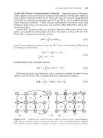
3.3
In a classic diffusion experiment, Darken welded an Fe-C alloy and an
Fe-
C-Si alloy together and annealed the resulting diffusion couple for
13
days at
1323
K,
producing the concentration profile shown in Fig. 3.11 [23]. Initially,
the C concentrations in the two alloys were uniform and essentially equal,
whereas the Si concentration in the Fe-C-Si alloy was uniform at about 3.8%.

After
a
diffusion anneal, the
C
had diffused “uphill” (in the direction of its
concentration gradient) out of the Si-containing alloy. Si is a large substi-
tutional atom,
so
the Fe and Si remained essentially immobile during the
6
0.6
e
+
0.5
2
%
0.4
cu
0
C
a,
E
0-l

0.3
Ill1
-20
-10
0
10

20
Distance
from
weld
(mm)
Figure
3.11:
Nonuniform concentration of C produced by diffusion from an initially
uniform distribution. Carbon migrated from the Fe-Si-C (left)
to
the Fe-C alloy (right).
From
Darken
[23].
70
CHAPTER
3:
DRIVING
FORCES
AND
FLUXES
FOR
DIFFUSION
diffusion, whereas the small interstitial
C
atoms were mobile. Si increases the
activity of
C
in Fe. Explain these results in terms of the basic driving forces
for diffusion.

Solution.
As
the
C
interstitials are the only mobile species, Eq. 3.35 applies, and
therefore
J;
=
-L11Vp1
(3.94)
(3.95)
Using the standard expression
for
the chemical potential,
p1
=
py
+
kTlna1
where
a1
=
71x1
is the activity
of
the interstitial
C,
(3.96)
The coefficient
L11

in Eq. 3.96 is positive and the equation therefore shows that the
C
flux will be in the direction
of
reduced
C
activity. Because the
C
activity is higher in
the Si-containing alloy than in the non-Si-containing alloy at the same
C
concentration,
the uphill diffusion into the non-Si-containing alloy occurs as observed. In essence, the
C
is pushed out
of
the ternary alloy by the presence
of
the essentially immobile Si.
3.4
Following Shewmon, consider the metallic couple specimen consisting of two
different metals,
A
and
B,
shown in Fig.
3.12
[18].
The bonded end is at
temperature

TI
and the open end is at
T2.
A mobile interstitial solute is
kJ/mol in one leg and
QFans
=
0
in the other. Assuming that the interstitial
concentration remains the same at the bonded interface at
TI,
derive the
equation for the steady-state interstitial concentration difference between the
two metal legs at
Tz.
Assume that
TI
>
T2.
present at the same concentration in both metals for which
QYans
=
-
84
r 1
Figure
3.12:
Metallic couple specimen made
up
of metals

A
and
B.
Solution.
In the steady state, Eq. 3.60 yields
CiQYans
VT
VCl
=
-~
kT2
Reducing to one dimension and integrating,
Therefore,
(3.97)
(3.98)
(3.99)
EXERCISES
71
Therefore, for leg
A,
(3.100)
while for leg
B,
cf(T2)
=
cf(T1).
Finally, because
cf(T1)
=
$(Ti)

=
cf(T2)
ci(Ti),
(3.101)
1
-l>
-84000
(Ti
-
T2)
Ac1
=
cl(T1)
exp
{
[
NokTiTz
3.5
Suppose that a two-phase system consists
of
a fine dispersion
of
a carbide
phase in a matrix. The carbide particles are in equilibrium with
C
dissolved
interstitially in the matrix phase, with the equilibrium solubility given by
c1
=
c,e

o
-AH/(kT)
(3.102)
If
a
bar-shaped specimen of this material is subjected to a steep thermal
gradient along the bar,
C
atoms move against the thermal gradient (toward
the cold end) and carbide particles shrink at the hot end and grow at the cold
end, even though the heat
of
transport is negative! (For an example, see the
paper by Mehmut et al.
[24].)
Explain how this can occur.
0
Assume that the concentration of
C
in the matrix is maintained in local
equilibrium with the carbide particles, which act as good sources and
sinks for the
C
atoms. Also,
AH
is positive and larger in magnitude
than the heat
of
transport.
Solution.

Ea.
3.102.
and therefore
The local
C
concentration will be coupled to the local temperature by
dcl
-
dci
dT
-
AH dT
I
dx dT dx kT2 dx
-

-
Substitution
of
Eq.
3.103
into Eq.
3.60
then yields
Jl
=

D1cl
(AH
+

Qtrans)
dz
dT
kT2
(3.103)
(3.104)
Because
(AH
+
Qtrans)
is
positive, the
C
atoms will be swept toward the cold end, as
observed.
3.6
Show that the forces exerted on interstitial atoms by the stress field
of
an edge
dislocation are tangent to the dashed circles in the directions of the arrows
shown in Fig.
3.8.
Solution.
The hydrostatic stress on an interstitial in the stress field
is
given by Eq.
3.80
and the force
is
equal to

=
-0lVP.
Therefore,
(3.105)
where
A
is a positive constant. Translating the origin of the
(x’,
y’)
coord+inate system
to a new position corresponding to
(2’
=
R,y’
=
0),
the expression for
Fl
in the new
(x,
y)
coordinate system is
72
CHAPTER
3:
DRIVING
FORCES
AND
FLUXES
FOR

DIFFUSION
Converting to cylindrical coordinates,
1
r
sin
8
$1
=
-R1
AV
[rZ+R2+2rRc~~B
The gradient operator in cylindrical coordinates
is
d
ld
V
=fir-+Ce
dr
T
de
(3.107)
(3.108)
Therefore, using
Eq.
3.107 and
Eq.
3.108 yields
$1
=
-

01
A
{fir(Rz
-r2)sin8+fie
[(R2
+r2)cose+2Rr]}
(3.109)
The force on an interstitial lying on a cylinder of radius
R
centered on the origin where
[RZ
+
r2
+
2Rr cos
el2
r
=
R
is then
(3.110)
The force anywhere on the cylinder therefore lies along
-60,
which is tangential to the
cylinder in the direction of decreasing
0.
3.7 Consider the diffusional flux in the vicinity of an edge dislocation after it
is
suddenly inserted into a material that has an initially uniform concentration
of interstitial solute atoms.

(a)
Calculate the initial rate at which the solute increases in a cylinder that
has an axis coincident with the dislocation and a radius
R.
Assume that
the solute forms a Henrian solution.
(b)
Find an expression for the concentration gradient at a long time when
mass diffusion has ceased.
Solution.
(a) The diffusion
flux
is given by
Eq.
3.83. Initially, the concentration gradient
is
zero
and the
flux
is due entirely to the stress gradient. Therefore,
hkT(1
-
v)
1
r2
-'
Now, integrate the
flux
entering the cylinder, noting that the
B

component con-
tributes nothing:
Rd9
=
0
2x
Asin6
(3.112)
where
A
=
constant. Note that this result can be inferred immediately, due to
the symmetry of the problem.
(b) When mass flow has ceased, the
flux
in
Eq.
3.83 is zero and therefore
vc1=
-
7:;;;;
t
yVlb
[-1
]
(3.113)
3.8
The diffusion of interstitial atoms in the stress field of a dislocation was con-
sidered in Section
3.5.2.

Interstitials diffuse about and eventually form an
sine cos0
~
Cr
+
Tue
r
EXERCISES
73
equilibrium distribution around the dislocation (known as a Cottrell atmo-
sphere),
which is invariant with time. Assume that the system is very large
and that the interstitial concentration is therefore maintained at a concentra-
tion
cy far from the dislocation. Use Eq. 3.83 to show that in this equilibrium
atmosphere, the interstitial concentration on a site where the hydrostatic
pressure,
P, due to the dislocation is
cyl
=
Cle
0
-nlp/(W
(3.114)
Solution.
According to Eq. 3.83,
(3.115)
At equilibrium,
=
0

and therefore
lncyq
+
=
a1
=
constant (3.116)
kT
Because cyq
=
c?
at
large distances from the dislocation where
P
=
0,
a1
=
In&,
Ceq
1-
-
C;e-%P/(kT)
(3.117)
3.9 In the Encyclopedia
of
Twentieth Century Physics,
R.W.
Cahn describes A.H.
Cottrell and B.A. Bilby's result that strain aging in an interstitial solid solu-

tion increases with time as
t213
as the coming of age of the science of quan-
titative metallurgy
[25].
Strain aging is a phenomenon that occurs when
interstitial atoms diffuse to dislocations in a material and adhere to their
cores and cause them to be immobilized. Especially remarkable is that the
t213
relation was derived even before dislocations had been observed.
Derive this result f0r an edge dislocation in an isotropic material.
0
Assume that the degree of the strain aging is proportional to the number
of interstitials that reach the dislocation.
0
Assume that the interstitial species is initially uniformly distributed and
that an edge dislocation is suddenly introduced into the crystal.
0
Assume that the force, -RlVP, is the dominant driving force for inter-
stitial diffusion. Neglect contributions due to
Vc.
0
Find the time dependence of the number of interstitials that reach the
dislocation. Take into account the rate at which the interstitials travel
along the circular paths in Fig. 3.8 and the number of these paths fun-
neling interstitials into the dislocation core.
Solution.
The tangential velocity,
u,
of an interstitial tkaveling along

a
circular path
of radius
R
in Fig. 3.8 will be proportional to the force
F1
=
-fIlVP
exerted by the
dislocation. In cylindrical coordinates,
P
is
proportional to
sinO/r,
so
(3.118)
74
CHAPTER 3: DRIVING FORCES AND FLUXES
FOR
DIFFUSION
Therefore,
v
K
F1
LX
l/rz.
As
shown in Fig. 3.8,
v
at equivalent points on each circle

will scale as
l/r*,
and because
r
at these points scales as
R,
1
(3.119)
The averagewelocity,
(v),
around each circular path will therefore scale as
l/RZ.
Since
the distance around a path is
2nR,
the time,
tR,
required to travel completely around
(3.120)
Therefore, at time,
t,
the circles with radii less than
Rcrit
K
t1/3
(3.121)
will be depleted of solute. During an increment of time
dt,
the average distance at
which interstitials along the active flux circles approach the dislocation is equal (to

a reasonable approximation) to
ds
=
(v)dt.
The total volume (per unit length of
dislocation) supplying atoms during this period is then
dV
LX
dt
Jm
(v)
dR
0:
Ldt
Lit
%it
(3.122)
where the integral is taken over only the active flux circles. Because the concentration
was initially uniform, the number
of
interstitials reaching the dislocation in time
t,
des-
ignated by
N,
is therefore proportional to the volume swept out. Therefore, substituting
Eq. 3.121 in Eq. 3.122 and integrating,
(3.123)
More detailed treatments are given in the original paper by Cottrell and Bilby
[25]

and
in the summary in Cottrell's text on dislocation theory
[22].
3.10
Derive the expression
+
DVCVPZ
JA
=

kT
for the electromigration
of
substitutional atoms in a pure metal, where
Dv
is
the vacancy diffusivity and
cv
is the vacancy concentration. Assume that:
There are two mobile components: atoms and vacancies.
Diffusion occurs by the exchange
of
atoms and vacancies.
There is a sufficient density
of
sources and sinks for vacancies
so
that
the vacancies are maintained at their local equilibrium concentration
everywhere.

Solution.
Vacancies are defects that scatter the conduction electrons and are therefore
subject to a force which in turn induces a vacancy current. The vacancy current results
in an equal and opposite atom current. The components are network constrained
so
that Eq. 2.21 for the vacancies, which are taken
as
the N,th component, is
Because
V~A
=
0
(see Eq. 3.64) and
pv
=
0,
EXERCISES
75
The vacancy current is therefore due solely to the_cross term arising from the current
of conduction electrons (which is proportional to
E).
The coupling coefFicient for the
vacancies is the off-diagonal coefficient
Lvq
which can be evaluated using the same
procedure as that which led to
Eq.
3.54
for the electromigration of interstitial atoms in
a metal. Therefore,

if
(CV)
is the average drift velocity of the vacancies induced by the
current and
Mv
is the vacancy mobility,
3.11
(a)
It is claimed in Section
C.2.1
that the mean curvature,
K,
of a curved
interface is the ratio of the increase in its area to the volume swept out
when the interface is displaced toward its convex side. Demonstrate this
by creating a small localized “bump” on the initially spherical interface
illustrated in Fig.
3.13.
I1
c
L
Figure
3.13:
Circular cap (spherical zone)
011
a
spherical interface.
(b)
Show that
Eq.

3.124
also holds when the volume swept out is in the form
of a thin layer of thickness
dw,
as illustrated in Fig.
3.14.
Figure
3.14:
with curvature
K
=
(1/R1)
+
(1/&).
Layer
of
thickness
diu
swept out
by
additioii
of
material
at
a11
interface
0
Construct the bump in the form of a small circular cap (spherical zone)
by increasing
h

infinitesimally while holding
r
constant. Then show that
dA
dV
/$=-
(3.124)
where
dA
and
dV
are, respectively, the increases in interfacial area and
volume swept out due to the construction of the bump.
76
CHAPTER
3:
DRIVING
FORCES
AND
FLUXES
FOR
DIFFUSION
Solution.
(a) The area of the circular cap in Fig. 3.13
is
A
=
7r
(T’
+

h2)
Here
T
and
h
are related to the radius of curvature of the spherical surface,
R,
by
the relation
R=?(l+$)
2h
(3.125)
The volume under the circular cap
is
given
by
7r
7r
V
=
-hr2
+
-h3
2
6
If
the bump is now created
by
forming a new cap of height
h

+
dh
while keeping
T
constant,
dA
=
27rhdh
(3.126)
(3.127)
Therefore, using
Eqs.
3.125, 3.126, and 3.127, and the fact that
h2/r2
<<
1,
dA
2
dV-RZK
-
-
(b)
The increase in area
is
dA
=
(R1
+
dw)
dB1

(Rz
+
dw)
dB2
-
R1
dB1
R2
dBz
=
(RI
+
Rz)
dw
dB1
dB2
The volume swept out
is
dV
=
Ri
dB1
Rz
dBz
dw
Therefore,
dA
1 1
_-
-

-+-=K
dV Ri Rz
CHAPTER
4
THE DIFFUSION EQUATION
The diffusion equation is the partial-differential equation that governs the evolution
of the concentration field produced by a given flux. With appropriate boundary
and initial conditions, the solution to this equation gives the time- and spatial-
dependence of the concentration. In this chapter we examine various forms assumed
by the diffusion equation when Fick’s law is obeyed for the flux. Cases where
the diffusivity is constant, a function of concentration, a function of time, or a
function of direction are included. In Chapter
5
we discuss mathematical methods
of obtaining solutions to the diffusion equation for various boundary-value problems.
4.1
FICK’S
SECOND
LAW
If the diffusive flux in a system is
f,
Section
1.3.5
and Eq. 1.18 are used to write
the diffusion equation in the general form
dC
+
_-
-n-V*J
at

where
n
is an added source or sink term corresponding to the rate per unit volume
at which diffusing material is created locally, possibly by means of chemical reaction
or fast-particle irradiation, and :is any flux referred to a V-frame. There frequently
are no sources or sinks operating, and
n
=
0
in Eq. 4.1. When Fick’s law applies
(see Section
3.1)
and
n
=
0,
Eq. 4.1 takes the general form
Kinetics
of
Materials.
By Robert W. Balluffi, Samuel
M.
Allen, and W. Craig Carter.
77
Copyright
@
2005
John Wiley
&
Sons, Inc.

78
CHAPTER
4
THE
DIFFUSION
EQUATION
dC
dt
-
-V
*
f=
V.
(DVc)
_-
which is sometimes called
Fick’s
second law
(note that Fick’s second law is simply
a consequence of the conservation of the diffusing species).
Accumulation within a volume depends only on the fluxes at its boundary. For
example, in one dimension,
where
N
is the number of particles and
A
is the area through which the diffusion
occurs. In three dimensions,
where in the final integral,
I(?,

t)
is the time-dependent value of flux at the oriented
surface
dV
that bounds V. The geometrical interpretation in Fig. 4.1 shows how
c(z,
t)
changes locally; the equations above imply a conservation constraint for the
entire concentration field.
Because Eq. 4.2 has one time and two spatial derivatives, its solution requires
three independent conditions: an initial condition and two independent boundary
conditions. Boundary conditions typically may look like
C(T=
TB)
=
f(t)
=
cg(t)
or
f(~=
TB)
.
=
g(t)
=
JB(~)
(4.5)
where
RB
is the normal to the boundary and the initial conditions have the form

c(z,
y,
2,
t
=
to)
=
c(T,
t
=
to)
=
h(z,
y,
2)
=
h(F)
=
CO(5,
y,
2)
(4.6)
In Chapter 3, several different types of diffusivity were introduced for diffusion
in a chemically homogeneous system or for interdiffusion in a solution. In each case,
Fick’s law applies, but the appropriate diffusivity depends on the particular system.
The development of the diffusion equation in this chapter depends only on the form
of Fick’s law,
f=
-DVc.
D

is a placeholder for the appropriate diffusivity, just
as
f
and
c
are placeholders for the type of component that diffuses.
Equation 4.2 can take various forms, depending upon the behavior of
D.
The
simplest case is when
D
is constant. However, as discussed below,
D
may be a
function of concentration, particularly in highly concentrated solutions where the
interactions between solute atoms are significant. Also,
D
may be a function of
time: for example, when the temperature of the diffusing body changes with time.
D
may also depend upon the direction of the diffusion in anisotropic materials.
4.1.1
Methods to solve the diffusion equation for specific boundary and initial conditions
are presented in Chapter
5.
Many analytic solutions exist forthe special case Lhat
D
is uniform. This is generally
not
the case for interdiffusivity

D
(Eq. 3.25). If
D
does
not vary rapidly with composition, it can be replaced by successive approximations
of a uniform diffusivity and results in a
linearization
of the diffusion equation. The
Linearization
of
the Diffusion Equation
4.1:
FICK'S
SECOND
LAW
79
linearized form permits approximate models from known solutions. The diffusivity
is expanded about its average value,
DO,
as follows
where
Ac
=
c
-
(c),
and
The diffusion equation becomes
The lowest-order approximation for small
Ac

and small
lVcl
is
(4.9)
(4.10)
which is the diffusion equation for constant diffusivity.
4.1.2
For evolution of a temperature field during heat flow, an equation with the same
form as Eq. 4.2 arises:
Relation
of
Fick's Second Law to the Heat Equation
(4.11)
where
h
is the enthalpy density and
cp
is the heat capacity per unit volume. The
ratio
KIcp
is called the
thermal
daffusivaty,
K.
It is assumed that no enthalpy is
stored by a phase change and that
cp
is constant.
Therefore, any result that follows from considerations of the form of Fick's second
law applies

to
evolution of heat as well as concentration. However, the thermal and
mass diffusion equations differ physically. The mass diffusion equation,
dcldt
=
V
.
DVc,
is a partial-differential equation for the density of an extensive quantity,
and in the thermal case,
dTldt
=
V .
KVT
is a partial-differential equation for an
intensive quantity. The difference arises because for mass diffusion, the driving force
is converted from
a
gradient in a potential
Vp
to a gradient in concentration
Vc,
which
is
easier to measure. For thermal diffusion, the time-dependent temperature
arises because the enthalpy density is inferred from a temperature measurement.
80
CHAPTER
4:
THE

DIFFUSION
EQUATION
4.1.3
The rate of entropy production,
tr
(Eq.
2.19),
for one-dimensional diffusion becomes
Variational Interpretation
of
the
Diffusion Equation
.
kD
dc
.=&)
(4.12)
when the activity coefficient is independent of concentration. Localized changes in
c(x,
t)
affect the rate of total entropy production. How changes in the evolution of a
field affect
a
functional (such as an integral quantity like total entropy production)
is a topic in the calculus of variations
[l].
For
an adiabatic system, the rate of total entropy production
Stot
is

a
functional
of the concentration field
c(x),
(4.13)
The functional gradient of
Stot
indicates the function pointing in the “direction”
of fastest increase. Gradients depend on an inner product because
it
provides a
measure of “distance” for functions
[2].
One choice of an inner product for functions
is the
L2
inner product, defined by
(4.14)
J
so
the magnitude of a function is related to the integral of its square:
lp(x)l
=
(pp)l/’.
Note that least-squares data fits use this inner product.
The functional gradient of
F
(or gradient of a vector function) can be defined
by
GF,

and the inner product with a velocity field
v:
(4.15)
That is, of all possible functions
v(x),
those that are parallel, subject to choice
of norm or inner product, to
GF
give the fastest increase in
F.
For the entropy
production with
D
=
constant,
(4.16)
2kD
dC
dt
Integrating by parts,
(4.17)
x2
d2c dc dc dc
If the boundary conditions are zero
flux
or fixed composition, the last term vanishes.
Comparison with the
L2
inner product reveals that for evolution according to the
diffusion equation,

c(x,
t)
changes
so
that
Stot
(total entropy “acceleration”) is its
most negative. Thus, entropy production, which is always positive, decreases in
time
as
rapidly
as
possible when
dcldt
cc
-Gs,,,
cc
d2c/dx2.
4.2
CONSTANT
DlFFUSlVlTY
81
4.2
CONSTANT DlFFUSlVlTY
When
D
is constant, Eq. 4.2 takes the relatively simple form of the linear second-
order partial differential equation
dC
-

=
DV'C
at
(4.18)
Some
of
the major features of this equation are discussed below, and methods
of
solving it under
a
variety
of
boundary and initial conditions are described at length
in Chapter
5.
4.2.1
Geometrical Interpretation
of
the Diffusion Equation when Diffusivity
is
Constant
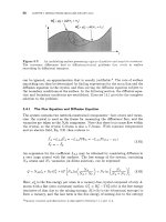
Figure 4.1 illustrates how a one-dimensional concentration field,
c(x,
t),
evolves ac-
cording to Eq. 4.18. The right-hand side
of
Eq. 4.18 is proportional to the curvature
of
the concentration profile. Where the curvature is negative,

as
on the left-hand
side, the concentration must decrease at a rate proportional to the magnitude
of
the curvature. Conversely, the concentration must increase on the right-hand side,
where the curvature is positive.
h
z
%-
v
X
Figure
4.1:
Evolut,ion
of
concentration
field
according to Fick's
law.
&/at
is
proportional
to
the curvature
of
the concentration
field.
4.2.2
Under certain conditions, boundary-value diffusion problems can be solved conve-
niently by scaling. First, introduce the dimensionless variable

q,
Scaling
of
the Diffusion Equation
(4.19)
2
q=-
rn
into the diffusion equation. Using Eq.
4.18
for
one-dimensional diffusion and
(4.20)
a
aq
a
a
av
a
at
at
aq
ax axaq
-
=

-
=

the diffusion equation becomes

(4.21)
82
CHAPTER
4:
THE
DIFFUSION
EQUATION
Next, suppose that for
the particular boundary-value problem under consideration,
the initial and boundary conditions are unchanged by scale change:
z=
Ax
t=
A2t
(4.22)
Then
77
is invariant under the scaling corresponding to Eq. 4.19 and
c
becomes
a function of the single variable,
v.
The diffusion equation becomes an ordinary
differential equation (i.e.,
d
+
d).
If
the boundary-value diffusion problem can be scaled according to Eq. 4.19, it is
considerably easier to solve. Consider the one-dimensional step-function diffusion

problem shown in Fig. 4.2, where
-m<x<o
{
::
o<x<m
c(x,t
=
0)
=
c(-co,t)
=
cL; C(co,t)
=
CR
(4.23)
The initial and boundary conditions given by Eq. 4.23 are transformed by scaling
into
c(-co) =cL
and
c(m) =c
R
(4.24)
and the diffusion equation has the form in Eq. 4.21. The entire boundary-value
diffusion problem is now rescaled. Equation 4.21 can be integrated by letting
dc
9'-
d7
Then
dq
-279

=
-
dv
which can be integrated to produce
where
a1
is a constant. Integrating again yields
(4.25)
(4.26)
(4.27)
(4.28)
Applying the step-function initial conditions in Eq. 4.24,
Figure
4.2:
One-dimensional step-function initial conditions.
lThe diffusion equation itself can always be rescaled. However, to solve
a
boundary-value diffusion
problem using the scaling method, the initial and boundary conditions must also be scalable.
4
z
CONSTANT
DIFFUSIVITY
83
where
a2
is
a
constant. The integral with the limit
x/m

is known as the
error
function,
abbreviated "erf"
:
(4.30)
The error function has the properties erf(0)
=
0,
erf(m)
=
1,
and erf(-z)
=
-erf(z).
So,
after evaluating
a2
by using the boundary conditions, the diffusion problem
posed above has the solution
(4.31)
where
C
=
(cR
+
cL)/2
and
Ac
=

cR
-
cL.
When c is assigned units
of
particles per
unit length, Eq.
4.31
describes the one-dimensional diffusion along
r
from
an
initial
step function on
a
line in one dimension
as
in Fig.
4.3~.
When
c
has units of particles
per unit area. it describes the one-dimensional diffusion from
a
step function in a
two-dimensional plane as in Fig.
4.3b,
and when the units are particles per unit
volume, it describes the one-dimensional diffusion from
a

step function in three
dimensions. as in Fig.
4.3~.
Figure
4.3:
diriierisioris.
Initial step-function distributions
iri
(a)
one,
(b)
two,
arid
(c)
three
Scaling as a Means
to
Compare Similar Systems.
When the diffusion problem is
invariant to the scaling parameter
ri
=
x/m. equal values
of
can be used
to determine relationships between length. time, and the value
of
the diffusivity.
For example. consider two masses that differ only in their length dimension. Let
the first block have length

L
and the second block have length
NL.
If
at a time,
7.
a
particular concentration appears at the center
of
the first block. the same
concentration will appear in the second block at time
o2r.
4.2.3
Superposition
Suppose that
~(x.
t) is a solution to the one-dimensional diffusion equation
(4.32)
84
CHAPTER
4:
THE
DIFFUSION
EQUATION
with boundary and initial conditions
p(~
=
a,
t)
=

Ap(t)
p(x
=
b,
t)
=
B,(t)
p(x,
t
=
0)
=
IP(x)
and that
q(x,
t)
is a solution to
(4.33)
(4.34)
with boundary and initial conditions
q(x
=
a,
t)
=
Aq(t)
q(x
=
b,
t)

=
Bq(t)
q(x,
t
=
0)
=
Iq(x)
(4.35)
Then, because the diffusion equation is a linear second-order differential equation,
T(X,
t)
=
p(x,t)
+
q(x,t)
is a solution for the boundary conditions and the initial
condition:
T(X
=
a,
t)
=
Ap(t)
+
Aq(t)
T(Z
=
b,
t)

=
Bp(t)
+
Bq(t)
T(X,
t
=
0)
=
Ip(x)
+
Iq(x)
(4.36)
The superposition of two solutions therefore also solves the diffusion equation with
superposed boundary and initial conditions.
Superposition of two displaced step-function initial conditions permits solutions
that describe diffusion from an initially localized source into an infinite domain.
The two step-function initial conditions in Fig. 4.4 have error-function solutions
(Eq. 4.31), and their superposition is a localized source of width
Ax.
The two step
functions are
-m<x<o
o<x<m
c(x,t
=
0)
=
and2
-W

<
x
<
AX
c(x,
t
=
0)
=
{
"0
Ax<x<m
(4.37)
(4.38)
-
-
co
x= Ax
Figure
4.4:
diffusion along
2.
'Although one initial condition is uiiphysical (i.e.,
a
negative concentration), the superposition
is physical and justifies its use. The negative concentration
is
similar to the use of
a
negative

electrical image charge to solve the electrostatics problem
of
the potential field produced by a
positive charge in a planar half-space where the plane bounding the half-space is held
at
zero
potential. The negative image charge outside the half-space allows superposition and satisfies the
boiindary condition at the plane bounding the half-space
[3].
Superposition method for coIistructing localized source for one-dimensional
4
3
DIFFUSIVITY
AS
A
FUNCTION OF
CONCENTRATION
85
Each step function evolves according to an error-function solution of the type
given by Eq. 4.31. and their superposition is
When
Ax
is small compared to the distance
x,
(4.40)
where the source strength,
nd,
is given by
When
c

is assigned units of particles per unit length,
nd
corresponds to the to-
tal number of particles in the source, and Eq. 4.40 describes the one-dimensional
diffusion from
a
point source as in Fig. 4.5~. Also, when c has units of particles
per unit area,
nd
has units of particles per unit length and
Eq.
4.40 describes the
one-dimensional diffusion in a plane in two dimensions from a line source initially
containing
nd
particles per unit length as in Fig.
4.5b.
Finally, when c has units
of particles per unit volume,
nd
has units of particles per unit area, and Eq. 4.40
describes the one-dimensional diffusion from a planar source in t’hree dimensions
initially containing
nd
particles per unit area as in Fig. 4.5~. These results are
summarized in Table 5.1.
Figure
4.5:
One-dirrierisiorial diffusion
into

an
infinite doriiaiii.
(a)
Point
source
diffusing
into
it
liric.
(b)
Line
soiircc diffusing into
a
plane.
(c)
Planar
source
diffusiiig into
a
volume.
4.3
DlFFUSlVlTY AS A FUNCTION OF CONCENTRATION
When
D
is
a
function
of
concentration [i.e.,
D

=
D(c)],
Eq.
4.2 takes the form
dC
dt

-
V.
[D(c)VC]
(4.42)
This differential equation is generally nonlinear [depending upon the form of
D(c)].
and solutions therefore can be obtained analytically only in certain special cases
which are not discussed here
[4].
86
CHAPTER
4:
THE
DIFFUSION
EQUATION
When Fick’s law applies, the concentration profile generally contains informa-
tion about the concentration dependence of the diffusivity.
For
constant
D,
step-
function initial conditions have the error function (Eq. 4.31) as
a

solution to
dc/dt
=
Dd2c/dx2.
When the diffusivity is
a
function of concentration,
dC d2c dD(c)
(8c)2
dt dx2 dc
-
=
D(c)-
+
-
(4.43)
For
identical initial conditions, the difference between
a
measured profile and the
error-function solution is related to the last (nonlinear) term in Eq. 4.43. When
diffusivity is
a
function of local concentration, the concentration profile tends to
be relatively flat at
a
concentration where
D(c)
is large and relatively steep where
D(c)

is small (this is demonstrated in Exercise 4.2). Asymmetry of the diffusion
profile in
a
diffusion couple is an indicator of
a
concentration-dependent diffusivity.
Matano developed
a
graphical method which, for certain classes of boundary
value problems, relates the form of the diffusion profile with the concentration de-
pendence of the interdiffusivity,
E(c),
introduced in Section 3.1.3
[5].
This method
can determine
6(c)
from the diffusion profile in chemical concentration-gradient dif-
fusion experiments where atomic volumes are sufficiently constant
so
that changes
in overall specimen volume are insignificant and diffusion can be formulated in
a
V-frame. The method uses scaling, as discussed in Section 4.2.2.
Consider
a
case where the initial and boundary conditions for a diffusion couple
are
-00<x<o
{

:I
o<x<00
c(x,t
=
0)
=
c(-m,t)
=
c:
C(00,t)
=
c1
R
Using the scaling parameter
q
=
x/&,
the diffusion equation becomes
(4.44)
(4.45)
and the initial and boundary conditions become
c1(q
=
00)
=
c?
c1(q
=
-00)
=

c1
L
(4.46)
Equation 4.45 can be integrated
as
(4.47)
If
c1
is
a
monotonically increasing function, variables can be changed
so
that
If
the profile is measured
at
some particular time
t
=
7,
x
=
q&?,
so
(4.48)
(4.49)
4.4:
DIFFUSIVITY
AS
A

FUNCTION
OF
TIME
87
because
dcl/dx(cl
=
cF)
=
0.
Equation 4.49 is an equation for
6
in terms of
integrals and derivatives of the function
q(x)
and its inverse
x(c~),
which can be
determined from a measured profile. The boundary condition
(4.50)
determines the position of the original interface (commonly termed the
Matano
interface)
where x
=
0
(Exercise 4.1 demonstrates this). The expression for the
interdiffusivity is
(4.51)
Equation 4.51 is an integral equation that can be used to determine

E(c1)
by a
graphical construction or numerical solution. The derivative required in Eq. 4.51
is provided by the measured concentration profile
at
time
r
and the integration is
performed on the inverse of
q(z)
[6].
However, this historically important method
is only moderately accurate, and
it
would be preferable to obtain diffusion profiles
for various assumed diffusivities as a function of concentration by computation.
D(c) could be deduced by fitting calculated results for a parametric representation
of
6(c)
to an experimentally determined diffusion profile.
4.4
DlFFUSlVlTY
AS
A
FUNCTION OF TIME
When
D
is a function of time, but not position, Eq. 4.2 takes the form
dC
-

=
V. [D(t)Vc]
=
D(t)V2c
at
(4.52)
This could be the case for a diffusion specimen that is slowly cooled while a uniform
temperature is maintained. Problems of this type can be treated by making the
change of variable
t
TO
=
Jd
D(t’)
dtl
(4.53)
Then
dc/dt
=
(dc/dTD)(dTD/dt)
=
(dC/dTD)D(t)
and Eq. 4.52 is transformed to
dC
-
=
v2c
drD
(4.54)
with the solution

c
=
c(x,r~)
for unit diffusivity. Equation 4.54, with the same
form as Eq. 4.18, holds when D is uniform. If the boundary conditions for a
time-dependent diffusivity problem are invariant under this change of variable,
so-
lutions from known constant-D problems can be applied to the time-dependent D
case. Consider, for example, the boundary-value problem in Fig. 4.2, which for
the constant-D case was solved by Eq. 4.31. Because
TD
=
0
when t
=
0,
the
initial and boundary conditions are invariant under the change of variable, and the
88
CHAPTER
4:
THE
DIFFUSION EQUATION
solution is
4.5
DlFFUSlVlTY
AS
A
FUNCTION OF DIRECTION
(4.55)

In the expressions for Fourier's law of heat conductivity and Fick's law for niass flux,
it
has been assumed that the flux vector is always parallel to the driving force vector.
However, these vectors are
not
parallel for general materials. For instance, consider
a bar. made of alternating layers of copper and silica glass, which
is
conducting heat
from
a
reservoir at high temperature to one of lower temperature, as in Fig. 4.6.
Because copper's heat conductivity is more t,han 60 times greater than silica's, the
temperature along each inclined copper sheet will be nearly uniform. Furthermore,
because the thermal gradient is always normal to lines of uniform temperature,
it points in
a
direction approximately normal to the copper sheets. However, the
heat flux is parallel to the bar because the only sources and sinks for heat are the
reservoirs
at
the ends.
This hypothetical example is similar to the case of a graphite single crystal.
Graphite has
a
hexagonal Bravais lattice. Along the basal planes, the carbon bond-
ing is covalent,
so
the thermal conductivity is
K11

=
355
J
m-'
s-'
K-*
,
nearly that
of carbon-diamond. Between the graphite layers, where the bonding is very weak,
the conductivity is much lower,
Kl
=
89.3 Jm-ls-l
K-l
.
F
igure 4.6 is therefore
representative of single-crystal graphite, where the basal plane is parallel to the
layers shown.
In general, the properties of crystals and other types of materials, such as com-
posites, vary with direction (i.e., macroscopic materials properties such as mass
diffusivity and electrical conductivity will generally be anisotropic). It is possible
to generalize the isotropic relations between driving forces and fluxes to account for
High conductivity
Low
conductivity
Figure
4.6:
Tlierrrial conduction in
a

laminar composite. The macroscopic value
of
the
thermal conductivity depends on the individual
values
of
conductivity
for
the
materials as
well
as
the inclination
of
the larriiriates.
4
5
DIFFUSIVITY
AS
A
FUNCTION
OF
DIRECTION
89
Dll
-
Dl2
Dl3
det D12 022
-

X
023
Dl3
023
033
-
ani~otropy.~ The isotropic form for Fick’s law is
f=
-DVc
Ji
=
-
=
0
(4.62)
dC
D-
dXi
(4.56)
where the final expression represents three equations, one for each coordinate axis,
written in component form. For the anisotropic case, there is a linear relation
between the flux and gradient vectors.
As
discussed in Section 1.3.7, the matrix of
the linear coefficients depends on the particular material and the orientation of the
material with respect to the V-frame:
or in component form,
dC
J~
=

ED^^
3
8%
or simply,
f=
-DVc
(4.58)
(4.59)
D
is called the diffusivity tensor and acts as an object that
connects
one vector
to another (e.g., the flux vector with the gradient vector). This connection can be
written in matrix form as in Eq. 4.57. The diffusivity tensor
D
is symmetric (i.e.>
Dij
=
Dji)
for any underlying material symmetry.
The anisotropic form of Fick’s law would seem to complicate the diffusion equa-
tion greatly. However, in many cases, a simple method for treating anisotropic
diffusion allows the diffusion equation to keep its simple form corresponding to
isotropic diffusion. Because
Daj
is symmetric, it is always possible to find a linear
coordinate transformation that will make the
Dij
diagonal with real components
(the eigenvalues of D). Let elements of such

a
transformed system be identified by
a
“hat.” Then
.=[
;
i3]
(4.60)
The diagonal elements of
b
are the eigenvalues of
D,
and the coordinate system
of
b
defines the
principal axes
21,22,
23
(the eigensystem). In the principal axes
coordinate system, the diffusion equation then has the relatively simple form
B,,
0
0
90
CHAPTER
4:
THE DIFFUSION EQUATION
If
&

is the matrix that rotates the original
(21, 22, x3)
coordinate system into the
principal
(21,22,23)
system, then according to Eq. 1.36,
fi
must be related to
D
D
=
RDR-l
(4.63)
To solve the diffusion equation in the principal coordinate system (i.e., Eq. 4.61),
the Cartesian space can now be stretched or contracted along the principal axes by
scaling:
by
(4.64)
A1/2
This scaling conserves the volume. Using Eq. 4.64, the diffusion equation can now
be written in terms of the
&:
(4.65)
where
V
=
(611fi22fi33)1/3.
Equation 4.65 has the same form
as
Fick’s second law

for a material with a constant isotropic diffusivity. Thus, known solutions to the
diffusion equation for constant isotropic diffusivity can be used to find solutions for
anisotropic constant diffusivities by a simple algorithm.
A
solution to Eq. 4.65 with
ID
and coordinates
[1,<2,[3
is rescaled back to the the principal axis coordinates
21
,
22,23
using Eq. 4.64. If necessary, the system can be transformed back into the
original, anisotropic laboratory coordinate system with
D
=
&-‘DB.
The diffusivity tensor has special forms for particular choices
of
coordinate axes if
the diffusing body itself has special symmetry (e.g., if it is crystalline).
Neumann’s
principle
states:
The symmetry elements
of
any physical property
of
a material must include
the symmetry elements of the point group

of
the materiaL4
A
consequence of Neumann’s symmetry principle is that direct tensor Onsager
coefficients (such as in the diffusivity tensor) must be symmetric. This is equivalent
to the addition
of
a center of symmetry (an inversion center) to a material’s point
group. Thus, the direct tensor properties of crystalline materials must have one
of
the point symmetries
of
the
11
Laue groups. Neumann’s principle can impose
additional relationships between the diffusivity tensor coefficients
Dij
in Eq. 4.57.
For a hexagonal crystal, the diffusivity tensor in the principal coordinate system
has the form
D11
0 0
(4.66)
4This also applies to the macroscopic properties of composite materials with underlying
symmetry-like honeycomb, wood, and woven materials-for which the crystal structure, if any,
may play no direct role.
EXERCISES
91
when
ig

lies along the crystal's c-axis arid
il
and
i2
lie anywhere in the basal
plane. Exercise
4.6
demonstrates that the diffusivity tensor in a cubic crystal has
the form
ro
0
01
(4.67)
and that the diffusion is therefore isotropic. Forms of the diffusivity tensor
D
for
other crystal systems are tabulated in Nye's text
[7].
Bibliography
1.
2.
3.
4.
5.
6.
7.
8.
I.M.
Gelfand and S.V. Fomin.
Calculus

of
Variations.
Prentice-Hall, Englewood Cliffs,
NJ.
1963.
W.C.
Carter,
J.E.
Taylor, and J.W. Cahn. Variational methods for microstructural
evolution.
JOM,
49(12):30-36.
1997.
P.M.
Morse and
H.
Feshbach.
Methods
of
Theoretical Physics,
Vols.
1
and
2.
McGraw-
Hill, New York, 1953.
J.
Crank.
The Mathematics
of

Diffusion.
Oxford University Press, Oxford, 2nd edition.
1975.
C.
hlatano. On relation between diffusion coefficients and concentrations of solid metals
(the nickel-copper system).
Jpn.
J.
Phys.,
8(3):109-113, 1933.
P.
Shewmon.
Diffusion
in
Solids.
The Minerals, Metals and Materials Society, War-
rendale, PA,
1989.
J.F. Nye.
Physical Properties
of
Crystals.
Oxford University Press, Oxford, 1985.
L.C.C. Da Silva and R.F. hlehl. Interface and marker movements in diffusion in solid
solutions of metals.
Trans.
AIME,
191(2):155-173, 1951.
EXERCISES
4.1

Consider the Boltzmann-hIatano analysis leading to Eq.
4.51.
Explain why
the condition imposed by Eq.
4.50
determines the location of the
x
=
0
plane
(i.e the position of the original interface).
Solution.
The laboratory coordinate system is used and there is no change in the overall
specimen volume. The integral in
Eq.
4.50
is
proportional to the sum
area
1
+
area
2
in Fig.
4.7.
Area
1
is positive and
area
2

is negative. When
z
=
0
is set at the position
of the original interface,
area
2
is proportional to the amount of diffusant that has left
0
X-
Figure
4.7:
Composition profile arising from interdiffusiori
92
CHAPTER
4:
THE
DIFFUSION
EQUATION
the original block of composition
cf,
and
area
1
is proportional to the amount that has
entered the original block of composition
cp.
Because these quantities must be equal,
the condition imposed by Eq.

4.50
determines the
z
=
0
plane.
4.2
The interdiffusivity,
5,
which measures the interdiffusion between Cu and Zn
in the laboratory frame, is a strong function of the concentration of Zn. The
curve describing
5(czn)
is concave upward and roughly parabolic in shape,
and
6(czn)
increases by a factor of about
20
when the Zn content increases
from
0
to 30 at.
%
[8].
Describe how the shape
of
the diffusion-penetration
curve for a diffusion couple made of Cu/CuSO at.
%
Zn is expected to deviate

from the symmetric form of the constant diffusivity error-function solution.
Solution.
Base your argument on the Boltzmann-Matano solution (Eq.
4.51),
which
links the interdiffusivity with the shape of the diffusion curve. Two factors are present:
the integral under the diffusion curve from
cz",
to the concentration in question,
czn,
and the reciprocal of the slope at
czn.
The integral varies from
0
at
z
=
00
to
0
at
z
=
-m
and reaches a maximum
at
z
=
0
(see Exercise

4.1).
The slope varies from
0
at
z
=
03
to
0
at
x
=
-m
and reaches a maximum somewhere in between. A little
trial and error quickly shows that the only way
D
can increase by a factor of
20
with
increasing
czn
with a difFusion curve of reasonable shape is to have a curve with a small
slope at high
CZ,,
and a large slope at low
czn.
Such a curve is markedly nonsymmetric
around its midpoint. Figure
4.8
shows an observed interdifFusion profile for this system.

30
0
-0.6
-0.4
-0.2
0
0.2
Distance
(cm)
Figure
4.8:
Silva
and
Mehl
[8].
Concentration profile observed in
Cu-30
at.
%
Zn diffusion couple.
From
Da
4.3
The Kirkendall effect can be studied by embedding an inert marker in the
original step-function interface
(x
=
0)
of the diffusion couple illustrated in
Fig.

3.4.
Show that this marker will move in the V-frame or, equivalently,
with respect to the nondiffused ends of the specimen, according to
x,
=
at1I2
where
cy
is a constant.
Solution.
According to Eq.
3.23,
the instantaneous velocity of any marker is given by
(4.68)