Nonimaging Optics Winston Episode 5 pot
Bạn đang xem bản rút gọn của tài liệu. Xem và tải ngay bản đầy đủ của tài liệu tại đây (545.72 KB, 30 trang )
are symmetrical transverse to the optic axis. As already noted in Section 6.4, the
étendue H generalizes to the difference of optical path lengths (up to an overall
constant). This remains true even in the presence of refractive media, provided
the optical path lengths are measured along rays. These rays need not be straight
lines. Thus, in Figure 6.14, the étendue H from Lambertian source AA¢ to section
PP¢ is proportional to [A¢P] - [AP], where the brackets indicate optical path
lengths. It follows that the lines of flow (indicated by arrows in the figure) lie along
contours of H = constant. Since the detailed balance condition holds in 2D, we may
construct concentrators by placing mirrors along the flow lines. However, it does
not follow that the 3D construction obtained by rotating the 2D flow line about the
optic axis will automatically satisfy detailed balance. Specific cases will have to be
checked with respect to detailed balance before the usefulness of the 3D designs
can be evaluated.
6.12 HAMILTONIAN FORMULATION
6.12.1 Introduction
The principles of Geometrical Optics can be formulated in several ways, all of them
being equivalent in the sense that they can provide the same information. Never-
theless, there are some particular problems for which one formulation is better
than the others—for example, the problem is more easily stated and sometimes
more easily solved using one of the formulations. This is common to disciplines
having more than one mathematical model. Probably, the most well-known
formulation of Geometrical Optics is the variational one (Fermat’s principle). In
Section 6.12.2 we will see another well-known formulation: the Hamiltonian equa-
tions. This formulation will be useful for stating and solving some nonimaging
design problems both in 2D and 3D geometry with the Poisson Brackets method.
This method is unique in the sense that it is able to give ideal designs in 3D geom-
etry in some cases. Unfortunately, the 3D designs obtained with this method
require graded refractive index materials, which limits its practical use.
The Hamiltonian formulation has been widely used in imaging optics. The
most important results are the characteristic functions and the simplicity with
which some optical invariants are recognized (see, for instance, Luneburg, 1964).
6.12 Hamiltonian Formulation 109
A
P
A¢
P
¢
Figure 6.14 Flow lines with refractive components AA¢ are a Lambertian source. The
arrows indicate row lines; the plain lines, rays.
One of these invariants is a common tool in nonimaging optics, the conservation
of étendue. Within the Hamiltonian formulation, this invariant is one of the
Poincaré’s invariants. Although Hamilton originally developed his equations for
optics, their applications in mechanics developed faster, so some of the results of
the theory may sound as if they belong to mechanics more than to optics. This may
be the case of the Poisson brackets. In other cases, the same result has two dif-
ferent names: one for optics and one for mechanics. For instance, in mechanics
Fermat’s principle is known as the principle of least action or the principle of
Maupertuis. The Hamiltonian formulation, when applied to nonimaging optics,
makes little use of the results for imaging optics, and because of this, its results
may appear more mechanic than optic.
6.12.2 Hamilton Equations and Poisson Bracket
As we will see, the Hamiltonian formulation is not unique. We start with the
description of the Hamilton equations that we will use in the most general form
we need. Let x
1
= x
1
(s), x
2
= x
2
(s), x
3
= x
3
(s), t = t(s) be the equations of a ray
trajectory in parametric form (s is the parameter) in the space x
1
- x
2
- x
3
- t (x
1
- x
2
- x
3
are the Cartesian coordinates, and t is the time). For each point of the
trajectory of a ray—that is, for each value of s, we have a value of the wave vector
k = (k
1
, k
2
, k
3
) and a value of the angular frequency w. Let k
1
= k
1
(s), k
2
= k
2
(s),
k
3
= k
3
(s), w = w(s) be the values of the three components of the wave vector and
the angular frequency, respectively. The set of eight functions x
1
= x
1
(s), x
2
= x
2
(s),
x
3
= x
3
(s), t = t(s), k
1
= k
1
(s), k
2
= k
2
(s), k
3
= k
3
(s), w = w(s) define a ray trajectory in
the phase space x
1
- x
2
- x
3
- t - k
1
- k
2
- k
3
- w. In general we are only interested
in the trajectory of the ray in the space x
1
- x
2
- x
3
, sometimes also including t.
The introduction of the other variables in this case is still interesting because they
simplify the formulation of the equations. The variables k
1
, k
2
, k
3
, - w are called
the conjugate variables of x
1
, x
2
, x
3
, t in the Hamiltonian formulation.
A key point of the Hamiltonian formulation is the so-called Hamiltonian func-
tion. In the case of optics, K(x
1
, x
2
, x
3
, t, k
1
, k
2
, k
3
, w) is a function such that K = 0
defines the surface of the wave vector k (Arnaud, 1974). The equation K = 0 is also
called Fresnel’s surface of wave normals, and it is directly related to the Fresnel’s
Differential Equation (Kline and Kay, 1965). The function K can be determined by
the properties of the medium where the rays are evolving.
The Hamiltonian equations can be written as
(6.4)
The solutions of this system of equations are sets of eight functions x
1
= x
1
(s), x
2
=
x
2
(s), x
3
= x
3
(s), t = t(s), k
1
= k
1
(s), k
2
= k
2
(s), k
3
= k
3
(s), w = w(s). It can be proved
that the solutions of this equation system are curves contained in the hyper-
dx
ds
K
k
dk
ds
K
x
dx
ds
K
k
dk
ds
K
x
dx
ds
K
k
dk
ds
K
x
dt
ds
Kd
ds
K
t
1
1
1
1
2
2
2
2
3
3
3
3
==
==
==
==
∂
∂
∂
∂
∂
∂
∂
∂
∂
∂
∂
∂
∂
∂w
w∂
∂
110 Chapter 6 The Flow-line Method for Designing Nonimaging Optical Systems
surfaces K = constant of the phase space x
1
- x
2
- x
3
- t - k
1
- k
2
- k
3
- w—that is,
the function K is a first integral of the system (Arnold, 1976). A function F(x
1
, x
2
,
x
3
, t, k
1
, k
2
, k
3
, w) is a first integral of the system of Eq. (6.4) if F is constant along
any ray trajectory—that is, dF/ds = 0. F is said to be a “constant of motion” in
mechanics (Abraham and Marsden, 1978; Leech, 1958). This can be written as
(6.5)
The total derivative of F with respect to s can be written as (using Eq. (6.4))
(6.6)
The right-hand side of Eq. (6.6) is called the Poisson bracket of F and K, and it is
noted by {F, K}. With this notation Eq. (6.6) can be written as dF/ds = {F, K}. Thus,
a function F is a first integral of the Hamiltonian system when {F, K} = 0. It is
easy to check that {K, K} = 0 and thus to conclude that the solutions of the system
of Eq. (6.4) are contained in hypersurfaces K = constant.
Not all the solutions of Eq. (6.4) represent ray trajectories. The ray trajecto-
ries in the phase space x
1
- x
2
- x
3
- t - k
1
- k
2
- k
3
- w are only the solutions of
this equation system that are consistent with K = 0—that is, the curves contained
in the hypersurface K = 0.
The equation of this hypersurface K = 0 can be expressed in different ways.
For instance, let f(x) be any function such that f(x) = 0 only if x = 0. Then f(K) =
0 represents the same surface as K = 0. It can be easily seen that if f(K) is used
as the Hamiltonian function instead of K in Eq. (6.4), then the same ray trajecto-
ries are obtained (with different parameterization) provided that df/dx π 0 when
x = 0. In particular, if we multiply the Hamiltonian function by a nonzero func-
tion, the solutions of the Hamiltonian system remain the same but with different
parameterization, that is, instead of getting x
1
= x
1
(s), x
2
= x
2
(s), x
3
= x
3
(s), t = t(s),
k
1
= k
1
(s), k
2
= k
2
(s), k
3
= k
3
(s), w = w(s), we would get another set x
1
= x
1
(s¢), x
2
=
x
2
(s¢), x
3
= x
3
(s¢), t = t(s¢), k
1
= k
1
(s¢), k
2
= k
2
(s¢), k
3
= k
3
(s¢), w = w(s¢) but still giving
the same phase space trajectories.
One useful property fulfilled by the solutions of the Hamiltonian system is
given by the Maupertius principle (in mechanics), also known as the least action
principle, which corresponds to the Fermat’s principle of optics (Arnold, 1974). In
terms of the Hamiltonian system of Eq. (6.4) this principle says that the integral
(6.7)
along the ray trajectories in the space x
1
, x
2
, x
3
, t is an extremal among all the
curves connecting point A and point B that also fulfill K = 0—that is, among the
curves whose trajectory in the phase space x
1
- x
2
- x
3
- t - k
1
- k
2
- k
3
- w is con-
tained in the hypersurface K = 0. A and B are two points of the space x
1
, x
2
, x
3
, t.
k dx k dx k dx dt
B
A
11 22 33
++-
Ú
w
dF
ds
F
x
K
k
F
k
dK
x
F
x
K
k
F
k
K
x
F
x
K
k
F
k
K
x
F
t
K
d
FK
t
=-+-+
+
∂
∂
∂
∂
∂
∂∂
∂
∂
∂
∂
∂
∂
∂
∂
∂
∂
∂
∂
∂
∂
∂
∂
∂
∂
∂
w
∂
∂w
∂
∂
11 11 22 22 33
33
dF
ds
F
x
dx
ds
F
k
dk
ds
F
x
dx
ds
F
k
dk
ds
F
x
dx
ds
F
k
dk
ds
F
t
dt
ds
Fd
ds
=++++
+++=
∂
∂
∂
∂
∂
∂
∂
∂
∂
∂
∂
∂
∂
∂
∂
∂w
w
1
1
1
1
2
2
2
2
3
3
3
3
0
6.12 Hamiltonian Formulation 111
In other words, choose any curve of the space x
1
, x
2
, x
3
, t connecting A and B. Now
choose arbitrary functions k
1
= k
1
(x
1
, x
2
, x
3
, t), k
2
= k
2
(x
1
, x
2
, x
3
, t), k
3
= k
3
(x
1
, x
2
, x
3
,
t), w = w(x
1
, x
2
, x
3
, t) such that the Hamiltonian K vanishes along the curve. If these
functions are compatible with the solution of the Hamiltonian system of Eq. (6.4),
then the integral in Eq. (1.7) is an extremal among the other possible choices
(Arnold, 1974). Observe that there is no restriction on the relationship of k
j
and
dx
j
/dt in this way to establish Fermat’s principle in contrast with the usual way
to present it. Nevertheless, it can be proved that both ways to present the princi-
ple are equivalent (Arnold, 1974).
We shall restrict the analysis to time-invariant isotropic media. In this case,
the surface of the wave vectors is a simple equation
(6.8)
where c
o
is the light velocity in vacuum and n(x
1
, x
2
, x
3
, w) is the refractive index
at the point x
1
, x
2
, x
3
for the angular frequency w (see Arnaud, 1976, and Kline and
Kay, 1965, for obtaining the Hamiltonian function in other cases). Because the
media is time-invariant, the Hamiltonian function does not depend on t and thus
the last equation of the Hamiltonian system Eq. (6.4) expresses that w is inva-
riant along any ray trajectory (dw/ds = 0). Thus, w is a first integral of the
Hamiltonian system in this case.
If w = constant and we are not interested in the dependence of t with the para-
meter s, then we only need the first six equations of the system. Furthermore, if
we make the change of variables p
j
= k
j
·c
o
/w a new Hamiltonian system is obtained
(6.9)
where the parameterization s now is not the same as before. The system of Eq.
(6.9) is also a Hamiltonian system for the independent variables x
1
, x
2
, x
3
, p
1
, p
2
,
p
3
(the last three variables are the conjugate variables of the first three ones).
Again, the ray trajectories are only the solutions of the system of Eq. (6.9) that
are consistent with P(x
1
, x
2
, x
3
, p
1
, p
2
, p
3
) = 0, being the Hamiltonian function P
(6.10)
Observe that now w is a constant and thus an independent analysis can be done
for each value of w. The variables p
1
, p
2
, p
3
are called the optical direction cosines
of a ray—that is, p
1
is n(x
1
, x
2
, x
3
) times the cosine of the angle formed by the
tangent to the ray trajectory with respect to the x
1
axis (p
2
and p
3
are defined in
a similar way with respect to the x
2
axis and the x
3
axis).
The Poisson bracket is defined in a similar way as before and the total
derivative of a function F(x
1
, x
2
, x
3
, p
1
, p
2
, p
3
) along the trajectories can also be
written as
Ppppnxxx∫++-
(
)
1
2
2
2
3
22
123
,,,w
dx
ds
P
p
dp
ds
P
x
dx
ds
P
p
dp
ds
P
x
dx
ds
P
p
dp
ds
P
x
1
1
1
1
2
2
2
2
3
3
3
3
==-
==-
==-
∂
∂
∂
∂
∂
∂
∂
∂
∂
∂
∂
∂
Kkkk
nxxx
c
o
∫++-
(
)
=
1
2
2
2
3
2
22
123
2
0
ww,,,
112 Chapter 6 The Flow-line Method for Designing Nonimaging Optical Systems
(6.11)
Thus, if F is a first integral of the Hamiltonian system, then it must fulfill {F, P}
= 0.
When the Hamiltonian function is a first integral (and it is so in all the for-
mulations that we have shown), then a new Hamiltonian system with two fewer
variables can be built up, provided that the equation P = 0 can be solved for one
variable (Arnold, 1974). Assume that this variable is p
3
. Then, the new formula-
tion of Hamilton equations is
(6.12)
The ray trajectories are now the solutions of the system, without restriction to
H = 0. The parameter of these ray trajectories is x
3
—that is, the conjugate vari-
able of p
3
in the system of Eq. (1.9). The function H is H =-p
3
when solved from
the equation P = 0—that is,
(6.13)
Eqs. (6.12) and (6.13) are the usual way in which Hamiltonian equations are intro-
duced in optics (Luneburg, 1964). Nevertheless, we won’t use it. For our purposes,
Eq. (6.9) with the condition P = 0 is a more convenient way to set the basic equa-
tions of Geometrical Optics.
Before going further, we still need a last system of Hamilton equations. This
is the one obtained when a change of variables from x
1
, x
2
, x
3
to a new set of orthog-
onal coordinates i
1
, i
2
, i
3
is done. This transformation belongs to a class of vari-
able transformations called canonical (Leech, 1958), and owing to this fact, the
Hamilton equations remain very similar (Leech, 1958; Miñano, 1986). Canonical
transformations are characterized by a “generating function” G. For our purposes
the expression of G is
(6.14)
where the functions i
1
, i
2
, i
3
in Eq. (6.14) give the values of the coordinates i
1
, i
2
, i
3
for a point x
1
, x
2
, x
3
·u
1
, u
2
, u
3
are the conjugate variables of i
1
, i
2
, i
3
. According to
the canonical transformation theory, the new conjugate variables can be expressed
as
(6.15)
The resulting Hamiltonian system is
p
p
p
i
x
i
x
i
x
i
x
i
x
i
x
i
x
i
x
i
x
u
u
u
1
2
3
1
1
2
1
3
1
1
2
2
2
3
2
1
3
2
3
3
3
1
2
3
Ê
Ë
Á
Á
ˆ
¯
˜
˜
=
Ê
Ë
Á
Á
Á
Á
Á
Á
ˆ
¯
˜
˜
˜
˜
˜
˜
Ê
Ë
Á
Á
ˆ
¯
˜
˜
∂
∂
∂
∂
∂
∂
∂
∂
∂
∂
∂
∂
∂
∂
∂
∂
∂
∂
Gxxxuuu uixxx uixxx uixxx
123123 11123 22123 33123
,,,,, ,, ,, ,,
(
)
=
(
)
+
(
)
+
(
)
Hnxxx pp∫-
(
)
2
123 1
2
2
2
,,,w
dx
dx
H
p
dp
dx
H
x
dx
dx
H
p
dp
dx
H
x
1
31
1
31
2
32
2
32
==-
==-
∂
∂
∂
∂
∂
∂
∂
∂
dF
ds
FP
F
x
P
p
F
p
P
x
F
x
P
p
F
k
P
p
F
x
P
p
F
p
P
x
=
{}
=-+-+-,
∂
∂
∂
∂
∂
∂
∂
∂
∂
∂
∂
∂
∂
∂
∂
∂
∂
∂
∂
∂
∂
∂
∂
∂
11 11 22 22 33 33
6.12 Hamiltonian Formulation 113
(6.16)
and the Hamiltonian function is
(6.17)
where a
1
, a
2
, and a
3
are, respectively, the modulus of the gradient of i
1
, i
2
, and
i
3
over the refractive index n (i.e., a
j
= |—i
j
|/n). Remembering the expressions of
the scale factors h
j
(Weisstein, 1999) of Differential Geometry, we can write a
j
=
1/(h
j
n). The refractive index n is in general a function of i
1
, i
2
, i
3
.
With the aid of Eq. (6.15) it is easy to find the physical meaning of the conju-
gate variables u
i
: A point i
1
, i
2
, i
3
, u
1
, u
2
, u
3
of the new phase space represents a
ray passing by the point i
1
, i
2
, i
3
with optical direction cosines a
1
u
1
, a
2
u
2
, a
3
u
3
with
respect to the three orthogonal vectors —i
1
, —i
2
, —i
3
. Figure 6.15 shows these three
orthogonal vectors and an arbitrary ray. The i
1
lines are given by equations i
2
=
constant, i
3
= constant. The i
2
, i
3
lines are defined in a similar way.
6.12.3 Optical Path Length
With the information provided in Figure 6.15 it is easy to see that the differential
of path length dL can be written as
(6.18)
Taking into account Eq. (6.17), the optical path length L
AB
of a ray is given by the
integral of Eq. (6.7) applied to our problem—that is,
dL
di
au
di
au
di
au
u di u di u di
au au au
====
++
++
1
1
2
1
2
2
2
2
3
3
2
3
11 22 33
1
2
1
2
2
2
2
2
3
2
3
2
H uaiii uaiii uaiii∫
(
)
+
(
)
+
(
)
-
1
2
1
2
123 2
2
2
2
123 3
2
3
2
123
1,, ,, ,,
di
ds
H
u
du
ds
H
i
di
ds
H
u
du
ds
H
i
di
ds
H
u
du
ds
H
i
1
1
1
1
2
2
2
2
3
3
3
3
==-
==-
==-
∂
∂
∂
∂
∂
∂
∂
∂
∂
∂
∂
∂
114 Chapter 6 The Flow-line Method for Designing Nonimaging Optical Systems
—i
2
—i
1
—i
3
ray
cos
-1
(a
3
u
3
)
cos
-1
(a
2
u
2
)
cos
-1
(a
1
u
1
)
i
1
-line
i
2
-line
i
3
-line
Figure 6.15 Physical meaning of the conjugate variables u
i
.
(6.19)
This integral is evaluated along a ray trajectory in the phase space. With Eq. (6.16)
we get
(6.20)
Taking into account Eq. (6.17),
(6.21)
Note that H = 0 for the ray trajectories. Eq. (6.21) provides the information we
need to understand the physical meaning of ds:
1
/
2
of the optical path length dif-
ferential dL. It should be remembered that the parameterization of the ray tra-
jectory, and thus the physical meaning of s, is associated with the Hamiltonian
function we are using.
6.13 POISSON BRACKET DESIGN METHOD
The Poisson bracket design method is, as yet, one of the few known 3D nonimag-
ing concentrator design methods. In general, this method provides concentrators
requiring variable refractive index media, which is impractical in most of the cases.
The main interest of the Poisson bracket method is that it provides ideal 3D con-
centrators, and thus it proved that such ideal concentrators exist. In particular,
we will design a 3D maximal concentrator illuminated by a bundle of rays having
an angular spread q with respect the entry aperture’s normal, that is, the set of
rays that are concentrated are formed by all the rays that impinge a flat entry
aperture forming an angle smaller than a certain value q with the normal to this
aperture. The concentrator has maximal concentration, and thus the ratio of entry
to exit apertures areas is n
2
/sin
2
q, where n is the refractive index of the points of
the exit aperture, which is the same for all of them. Figure 6.16 shows a scheme
of such a concentrator.
The work presented here was developed some years ago (Miñano, 1985b;
1985c; Miñano, 1993a; 1993b; Miñano and Benítez, 1999). Some nontrivial ideal
3D nonimaging concentrators were already known when the Poisson brackets
method was developed. Among these, the most important is the hyperboloid of rev-
olution (Winston and Welford, 1979). Figure 6.17 shows one of these concentra-
tors. A reflector whose cross-section is a hyperboloid forms it. The foci of this
hyperboloid generate the circumference C when the cross-section is rotated around
the axis of revolution symmetry. If the inner side of the hyperboloid of revolution
is mirrored, then it becomes an ideal nonimaging concentrator with the following
definitions of the input and output bundles: The input bundle is formed by all the
rays crossing the entry aperture that would reach any point of the circle C (virtual
receiver) if there was no mirror. The set of rays crossing the exit aperture forms
the output bundle. The concentrator is ideal in the sense that any ray of the input
L H ds ds
AB
B
A
B
A
=+
(
)
=
ÚÚ
21 2
Lu
di
ds
u
di
ds
u
di
ds
ds u
H
u
u
H
u
u
H
u
ds
AB
B
A
B
A
=++
Ê
Ë
ˆ
¯
=++
Ê
Ë
Á
ˆ
¯
˜
ÚÚ
1
1
2
2
3
3
1
1
2
2
3
3
∂
∂
∂
∂
∂
∂
L u di u di u di
AB
B
A
=++
Ú
11 22 33
6.13 Poisson Bracket Design Method 115
bundle is transformed in a ray of the output bundle by the concentrator, and any
ray of the output bundle comes from a ray of the input bundle. Thus, the same
rays form both bundles. The only difference is that the input bundle describes the
transmitted bundle at the entry aperture and the output bundle describes it at
the exit aperture. Additionally, the concentrator has maximal concentration
because the output bundle comprises all the rays crossing the exit aperture, and
thus the exit aperture has the minimum possible area such that all the rays of the
transmitted bundle cross it.
From the preceding definition of ideal concentrator we can conclude that any
device may be an ideal concentrator with a proper definition of the input and
output bundles. Nevertheless, the name “ideal” used to be restricted to cases in
which both input and output bundles have a practical interest. There are two types
of bundle that deserve special attention.
1. Finite source. The rays of this bundle are those linking any point of a given
surface with any point of another given source (see Figure 6.18).
2. Infinite source. This bundle can be described as formed by all the rays that
meet (real or virtually) a given surface forming an angle smaller than or equal
116 Chapter 6 The Flow-line Method for Designing Nonimaging Optical Systems
entry aperture
exit aperture
q
Figure 6.16 3D ideal concentrator designed to collect the rays impinging its entry aper-
ture with directions within a cone of angle q.
entry aperture
exit aperture
virtual receiver
C
axis
Figure 6.17 Hyperboloid of revolution as an ideal 3D concentrator.
q with a given reference direction. Then, this bundle is fully characterized by
the surface (also called aperture), by the angle q, and by the reference direc-
tion. This bundle is a typical input bundle for solar applications: The rays to
be collected are those reaching the concentrator aperture forming an angle
with the normal to this aperture smaller than the acceptance angle of the
system (see Figure 6.19).
The input bundle of the hyperboloid of revolution of Figure 6.17 is a finite source
where C
1
is the entry aperture and C
2
is the virtual receiver. The output bundle
is an infinite source of the type shown in Figure 6.19 with q = 90°.
A thin lens with focal length f can be considered as a concentrator whose input
bundle is an infinite source of angle q and whose output bundle is a finite source
of the type shown in Figure 6.18, C
1
being the lens aperture and C
2
being a circle
located at the focal plane with radius equal to f·tan(q). For a real lens this descrip-
tion is approximate. The approximation is better for smaller since q is smaller.
Therefore, a combination of a hyperboloid of revolution reflector and a thin lens
6.13 Poisson Bracket Design Method 117
C
2
C
1
aperture
q
Figure 6.18 Example of finite source. The rays of this bundle are those linking any point
of the circle C
1
with any point of the circle C
2
.
Figure 6.19 Example of infinite source of angle q. It can also be considered as a particu-
lar case of the bundle shown in Figure 6.18 when one of the circles is infinitely far from the
other and of infinite radius.
is, approximately, an ideal concentrator of the type shown in Figure 6.16 (at least
for small values of q) (Welford, O’Gallagher, and Winston, 1987), if the combina-
tion is done in such a way that the output bundle of the thin lens, which is the
finite source defined by the circles C
1
and C
2
, is made to coincide with the input
bundle of the hyperboloid (see Figure 6.20).
A characteristic of the hyperboloid of revolution as a nonimaging concentra-
tor is that its transmitted bundle is what we call an elliptic bundle. An elliptic
bundle is defined as one whose edge rays cross any point of the x
1
- x
2
- x
3
space
form—in this space, a cone with an elliptic basis. Figure 6.21 shows one of these
cones corresponding to the bundle of rays illuminating the circle C. This bundle
is of the elliptic type, and thus the rays form an elliptic cone at any point of the
space. The figure shows also two flow lines of this bundle.
If the elliptic bundle is such that its flow lines are the coordinate lines of a
three-orthogonal coordinate system (i
1
, i
2
, i
3
), then it can be easily proved that the
edge rays conjugate variables u
1
, u
2
, u
3
fulfill an equation like
118 Chapter 6 The Flow-line Method for Designing Nonimaging Optical Systems
thin lens
exit aperture
C
2
C
1
q
Figure 6.20 A thin lens combined with a hyperboloid of revolution behaves approximately
like an ideal 3D concentrator with maximal concentration for an infinite source subtending
an angle q.
flow line
elliptic cone
C
Figure 6.21 The edge rays of an elliptical bundle passing through a point form a cone with
an elliptical basis.
(6.22)
where the functions a
1
, a
2
, a
3
are arbitrary functions of i
1
, i
2
, i
3
. This equation,
together with Eq. (6.17) defines a conic curve (ellipse, parabola, or hyperbole) in a
u
n
- u
m
plane (n, m = 1, 2, 3, n π m). Note that it is necessary that Eq. (6.17) be
fulfilled because the rays are the solutions of the Hamiltonian system that are con-
sistent with H = 0, which is Eq. (6.17).
6.13.1 Statement of the Problem
The ray trajectories in the phase space x
1
- x
2
- x
3
- p
1
- p
2
- p
3
or (i
1
- i
2
- i
3
- u
1
- u
2
- u
3
) do not cross between them. This property, which derives from the unique-
ness of the solution of a system of first order differential equations passing through
a given point of the phase space is particularly useful for describing visually the
problem that we want to solve and comparing it with the typical synthesis problem
in imaging optics. For the purpose of describing qualitatively both problems, we
are going to consider a simplified case. This is when the rays are contained in a
plane (for instance the x
1
- x
2
). We call this case a 2D system, and it can be derived
from the general case by establishing ∂n/∂x
3
= 0 and p
3
= 0. In this case the phase
space can be limited to four variables x
1
- x
2
- p
1
- p
2
. Moreover, since the ray tra-
jectories are restricted to P = 0 (P is defined in Eq. (6.10)), then p
2
=±[n
2
(x
1
, x
2
) -
p
1
2
]
1/2
—that is, for each point x
1
, x
2
, p
1
there are only two possible values of p
2
such
that x
1
, x
2
, p
1
, p
2
describes a ray. Both values of p
2
give the same ray path (x
2
increases with the parameter s for one value of p
2
and for the other value x
2
decreases with increasing s). Thus, if we forget one of the two possible directions
of the ray, we can say that each ray can be fully characterized by a point x
1
, x
2
, p
1
.
Fortunately, these are only three variables, and the trajectories can be easily rep-
resented. For instance, Figure 6.22 shows the trajectory of a ray in the phase space
x
1
- x
2
- p
1
and its projection on the x
1
- x
2
plane. This projection has the equation
(6.23)
This ray trajectory is the one obtained for meridian rays in a fiber whose square
of the refractive index has a parabolic profile versus x
1
(see Miñano, 1985b).
A one-parameter family of ray trajectories in the phase space forms, in general,
a surface. For instance, consider the family of rays derived from Eq. (6.23) taken
C as the parameter of the family (A and B are kept constants). The representa-
tion of this family in the phase space are the cylinders shown in Figure 6.23. The
x A Bx C
12
=+
(
)
sin
uiiiuiiiuiii
1
2
1
2
123 2
2
2
2
123 3
2
3
2
123
1aaa,, ,, ,,
(
)
+
(
)
+
(
)
=
6.13 Poisson Bracket Design Method 119
x
2
x
1
p
1
Figure 6.22 Ray trajectory in the phase space x
1
- x
2
- p
1
(heavy line) and in the x
1
- x
2
plane.
ray trajectories in this phase space are wrapped around the cylinder, and they
don’t cross. Different cylinders correspond to different values of A and B.
Now let us consider the problem of designing a 2D nonimaging concentrator
in the phase space. In general the problem involves determining the optical system
such that a given bundle of rays described at a line called the entry aperture is
transformed by the optical system in another prescribed bundle of rays at the exit
aperture. Assume for simplicity that the entry aperture is at x
2
= 0 and that the
exit aperture is at x
2
= 1. The bundle at the entry aperture can be defined by a
region of the plane x
2
= 0, as well as the bundle at the exit aperture is defined by
another region of the plane x
2
= 1 (see Figure 6.24 and Miñano, 1993a). Because
of the conservation of étendue, both regions must have the same area.
The edge-ray principle simplifies the problem of design: To get the aforemen-
tioned goal we must design an optical system that transforms the edge rays of the
bundle at the entry aperture in the edge rays of the bundle at the exit aperture.
This is equivalent to stating that the edge rays’ trajectories will form a tubelike
surface in the phase space that cuts the x
2
= 0 plane and the x
2
= 1 plane at the
contours of the regions defining the bundles at the entry and at the exit.
120 Chapter 6 The Flow-line Method for Designing Nonimaging Optical Systems
p
1
x
1
x
2
Figure 6.23 Surfaces of the phase space representing three one-parameter bundles of rays.
Nonimaging
x
1
x
2
x
1
x
2
p
1
p
1
Figure 6.24 The nonimaging design problem: The bundles of rays at the entry aperture
(x
2
= 0) and at the exit aperture (x
2
= 1) are prescribed (left side). An optical system has to
be designed such that the edge rays at the entry are the same as the edge rays at the exit;
that is, the edge ray trajectories in the phase space must form a surface connecting the edge
rays’ representations at both apertures.
In general the imaging problem has less degrees of freedom. Figure 6.25 shows
the phase space representation for this case. At the object and at the image plane
there is a prescribed family of one-parameter bundles of rays to be coupled. The
rays issuing or reaching a point of the object or imaging planes form each one of
these one-parameter bundles. From the mathematical point of view, in the non-
imaging problem we have to find an optical system that admits a given particular
integral of the Hamilton equations, whereas in the image problem we have to find
an optical system that admits a given first integral of the Hamilton equations.
Now let us go back to the 3D case. Let us call restricted entry phase space to
the points of the phase space whose spatial coordinates x
1
, x
2
, x
3
belong to the entry
aperture. The restricted exit phase space is defined in a similar way. In the non-
imaging design the edge rays have prescribed descriptions in the restricted entry
and exit phase spaces. The edge rays in the restricted phase spaces form a curve
that encloses the set of points representing the rays of the transmitted bundle.
Note that in the 3D case, the edge rays form a three-parameter bundle of rays,
and thus their trajectories in the six-dimensional phase space (x
1
- x
2
- x
3
- p
1
-
p
2
- p
3
) form a four-dimensional subset that must be contained in the subset P(x
1
,
x
2
, x
3
, p
1
, p
2
, p
3
) = 0. The subset P = 0 is then five-dimensional, and thus a four-
dimensional subset can be characterized by an additional equation of the type w(x
1
,
x
2
, x
3
, p
1
, p
2
, p
3
) = 0 (w here has no relation with the angular frequency, which is
not considered in this analysis). The surface of the edge rays’ trajectories is then
defined by P = 0 together with w = 0. The function w(x
1
, x
2
, x
3
, p
1
, p
2
, p
3
) is not
uniquely determined except when w = 0.
The question now is to find the conditions on the function w so w is a surface
formed by ray trajectories. The answer is that the Poisson bracket of w and P
should be zero, when P = 0 and when w = 0—that is,
(6.24)
Remember that the Poisson bracket is defined as
(6.25)
w
∂w
∂
∂
∂
∂w
∂
∂
∂
, P
x
P
pp
P
x
jj jj
j
j
{}
=-
Ê
Ë
Á
ˆ
¯
˜
=
=
Â
1
3
ww,,PP
{}
===
(
)
000when and
6.13 Poisson Bracket Design Method 121
Object
plane
Image
plane
Imaging
x
1
x
2
x
1
x
2
p
1
p
1
Figure 6.25 The imaging problem: A family of one-parameter bundles of rays at the object
plane (x
2
= 0) and another one at the image plane (x
2
= 1) are prescribed (left side). An optical
system has to be designed such that each bundle at the object plane is imaged to its corre-
sponding bundle at the image plane.
Since the variable transformation from x
1
- x
2
- x
3
- p
1
- p
2
- p
3
to i
1
- i
2
- i
3
- u
1
- u
2
- u
3
is canonical, the problem can be easily established in the new variables:
Eq. (6.24) becomes (now w is a function of the variables i
1
, i
2
, i
3
, u
1
, u
2
, u
3
obtained
with the preceding transformation from the function w(x
1
, x
2
, x
3
, p
1
, p
2
, p
3
))
(6.26)
The Poisson bracket of the functions w and H is expressed with the new variables
as
(6.27)
We have now new tools to proceed with the design problem. For instance, we
can propose a function w that fulfills the contour conditions at the restricted entry
and exit phase spaces and apply Eq. (6.26) and find out the conditions on the
Hamiltonian function H (see Eq. (6.17)) and thus the conditions on the refractive
index distribution and on the modulus of the gradients of the coordinate variables
(more precisely, the conditions on the functions a
j
= |—i
j
|/n).
Because we are not completely free to choose the Hamiltonian function
(because, for instance, its dependence with the squares of the conjugate variables
must be linear if a three-orthogonal coordinate system is used), then choosing the
function w is not completely free either. In order to find the restrictions we must
impose to the function w, we must expand Eq. (6.27).
The problem is further simplified if we restrict the analysis to elliptic edge ray
bundles that can be defined by a couple of equations H = 0 (H is defined in Eq.
(6.17)) together with
(6.28)
Observe that with this restriction, w and H are both linear functions of the squares
of the conjugate variables u
1
, u
2
, u
3
. The definition of Eq. (6.28) implies that the
cone formed by the rays of the bundle passing through any point i
1
, i
2
, i
3
has three
planes of symmetry. Therefore, the flow lines of the bundle are one of the three
coordinate lines. Thus, we are restricting elliptic bundles to those whose flow lines
may be coordinate lines of a three-orthogonal system. This restriction implies, for
instance, that the flow lines are orthogonal to a family of surfaces and thus that
J·—¥J = 0 (J is the geometrical vector flux) which is not a necessary condition
for J. This restriction is not imposed in the analysis done further in this chapter
using the Lorenz geometry tools, where, nevertheless, the refractive index is
assumed to be constant.
The type of bundle given by Eq. (6.28) can be used as an edge ray bundle in
the flow-line design method where the existence of a reflector surface connecting
entry and exit apertures borders permits the edge ray bundle to be unbounded in
the spatial variables i
1
, i
2
, i
3
(see Appendix B). This won’t to be the case of the
Simultaneous Multiple Surface design method described in Chapter 8.
Owing to the symmetries of the elliptic bundles, if we find a refractive index
distribution that has as a solution a prescribed elliptic bundle, then we will easily
be able to design a concentrator with the flow-line method. All we will have to do
is choose a surface formed by flow lines of the bundle as reflector. In the definition
of elliptic bundles given by Eq. (6.28) it is implicitly established that one of the
waaa∫
(
)
+
(
)
+
(
)
-=uiiiuiiiuiii
1
2
1
2
123 2
2
2
2
123 3
2
3
2
123
1
0
,, ,, ,,
w
∂w
∂
∂
∂
∂w
∂
∂
∂
, H
i
H
uu
H
i
jj jj
j
j
{}
=-
Ê
Ë
Á
ˆ
¯
˜
=
=
Â
1
3
ww,,HH
{}
===
(
)
000when and
122 Chapter 6 The Flow-line Method for Designing Nonimaging Optical Systems
three coordinate lines are flow lines of the bundle and that the plane tangents to
the surfaces i
j
= constant (j = 1, 2, 3) at each point i
1
, i
2
, i
3
are planes of symme-
try of the bundle at this point. Assume, for instance, that the coordinate lines i
1
(i.e., the lines i
2
= constant i
3
= constant) are the flow lines of interest. Then, any
surface i
2
= constant will contain flow lines and its tangents are planes of sym-
metry of the bundle. Then, if the surface i
2
= constant is mirrored, the bundle result
is unaffected (from the collection point of view), and thus we will obtain the desired
concentrator provided the surface i
2
= constant defines the entry and exit aperture
of the concentrator according to our requirements. The concentrator will be formed
by a mirror with the i
2
= constant surface shape and the refractive index distribu-
tion. The mirror edges will define the shape of the entry and exit apertures. Addi-
tionally we know that the rotational hyperbolic concentrator is a solution of this
type, and thus we know that there is at least one solution for this problem.
The analysis of elliptic bundles may appear too restrictive, and that may be
so. Nevertheless, we have to take into account that the edge-ray bundle of any
nontrivial ideal 3D concentrator known at present is an elliptic bundle. Moreover,
the concept of an elliptic bundle can also be applied in 2D geometry (see Section
6.16), and in this case any edge-ray bundle can be viewed as an elliptic bundle.
Since the majority of design methods of nonimaging concentrators (other than the
Poisson brackets and the numerical methods) are actually 2D methods, we can
conclude that the concept of elliptic bundle is not so restrictive.
6.13.2 Elliptic Edge-Ray Bundle Analysis
Let us define the following vectors.
(6.29)
(6.30)
(6.31)
The vectors a and a depend solely on i
1
, i
2
, i
3
. Using this notation, equations
H = 0, w = 0 remain as
(6.32)
(6.33)
Note that for a given edge-ray bundle—that is, for a given surface (H = 0, w = 0)—
the vector a is not uniquely determined: Any vector
(6.34)
where m is an arbitrary parameter m π 1 defines the same edge-ray bundle. Eqs.
(6.32) and (6.33) must be independent—that is, a ¥ a π 0.
The equation {w, H} = 0 can be written as
(6.35)
Because only the power 2 of u
1
, u
2
, u
3
appears in the equations w = 0 and H = 0,
then if there is a point (i
1
, i
2
, i
3
, u
1
, u
2
, u
3
) belonging to w = 0 and H = 0 it is nec-
w
∂a
∂
∂
∂
∂
∂
∂
∂
, H
iu iu
jj jj
j
j
{}
∫◊ ◊
Ê
Ë
Á
ˆ
¯
˜
-◊
Ê
Ë
Á
ˆ
¯
˜
Ê
Ë
Á
ˆ
¯
˜
=
=
=
Â
u
u
a
au
a 0
1
3
aam a
1
=+ -
(
)
a
w ∫◊-=u a 10
H ∫◊-=ua 10
a ∫
[]
aaa
1
2
2
2
3
2
,,
a ∫
[]
aaa
1
2
2
2
3
2
,,
u ∫
[]
uuu
1
2
2
2
3
2
,,
6.13 Poisson Bracket Design Method 123
essary that the points (i
1
, i
2
, i
3
, ±u
1
, ±u
2
, ±u
3
) also belong to w = 0 and H = 0. Thus,
if {w, H} = 0 at (i
1
, i
2
, i
3
, u
1
, u
2
, u
3
), it is necessary that {w, H} = 0 also at (i
1
, i
2
, i
3
,
±u
1
, ±u
2
, ±u
3
). This means that the factors of odd powers of u
1
, u
2
, and u
3
in Eq.
(6.35) must be zero. From this result we obtain three equations instead of Eq.
(6.35).
(6.36)
These three equations together with Eqs. (6.32) and (6.33) should be satisfied by
a one-parametric set of vectors u at each point i
1
, i
2
, i
3
. Eqs. (6.32) and (6.33) are
assumed to be independent—that is, a ¥ a π 0. Thus, any of Eq. (6.36) must be a
linear combination of Eqs. (6.32) and (6.33)—that is, any T
j
must be parallel to
a - a:
(6.37)
From this result we get six differential equations involving the functions a
j
and
a
j
, which, surprisingly, can be combined so they become easily integrated:
(6.38)
(6.39)
Where the functions f
j,k
fulfill that ∂f
j,k
/∂i
j
= 0.
Eq. (6.47) can also be written as
(6.40)
Where 1 is the column vector (1, 1, 1) and [M] is the matrix
(6.41)
Since the matrix Eq. (45) must be satisfied by the vectors a and a, and these vectors
fulfill a ¥ a π 0, then the determinant of [M] must be zero (this equation could be
got directly from Eq. (6.39))
(6.42)
where the dependence on the variables i
1
, i
2
, i
3
has been explicitly written. Let us
rearrange this equation as follows:
(6.43)
Eq. (6.43) is a functional equation in which the left-hand side does not depend on
i
3
. If we fix a value of i
3
in the right-hand side, we get an equation that establishes
that the left-hand side is a product of a function of i
1
times a function of i
2
(see
Castillo, 1996; and Castillo and Ruiz-Cobo, 1992). Therefore, we can write the fol-
lowing equations:
-
(
)
(
)
=
(
)
(
)
(
)
(
)
fii
fii
fii
fii
fii
fii
31 1 2
32 1 2
13 2 3
12 2 3
21 1 3
23 1 3
,
,
,
,
,
,
,
,
,
,
,
,
fiifiifii fiifiifii
13 2 3 21 1 3 32 1 2 12 2 3 23 1 3 31 1 2
0
,,, ,,,
,,, ,,,
(
)
(
)
(
)
+
(
)
(
)
(
)
=
M
[]
=
È
Î
Í
Í
Í
˘
˚
˙
˙
˙
0
0
0
32 23
31 13
21 12
ff
ff
ff
,,
,,
,,
Ma M
[]
◊=
[]
◊=11a
a
aa
fjk kj
jj
jk jk
jk
22
22 22
123
-
-
== π
a
aa
,
,,,
∂
∂
aa
ai
aa
a
jk k j
j
jk jk
jj
22 22
22
0123
-
-
Ê
Ë
Á
ˆ
¯
˜
== π,,,
Ta
j
j¥-
(
)
==a 0123,,
u
a
uT◊-
Ê
Ë
Á
ˆ
¯
˜
∫◊ = =a
ii
j
j
j
j
j
j
22
0123
∂
∂
a
∂
∂
a
,,
124 Chapter 6 The Flow-line Method for Designing Nonimaging Optical Systems
(6.44)
where n
1
, n
2
, n
3
are three functions that only depend on one variable as specified;
that is,
(6.45)
Let us introduce the functions s
1
, s
2
, s
3
as
(6.46)
that is, s
j
fulfills
(6.47)
With these new functions Eq. (6.40) can be written as
(6.48)
where the vectors S and N are
(6.49)
(6.50)
From Eq. (6.48) it is concluded that
(6.51)
Expanding Eq. (6.51) with the definitions in Eqs. (6.49) and (6.50) and dividing
over n
1
(i
1
) n
2
(i
2
) n
3
(i
3
) we get a functional equation called the generalized Sincov’s
equation (Castillo, 1996; Castillo and Ruiz-Cobo, 1992). Its solution is
(6.52)
where V is a vector whose components fulfill
(6.53)
Introducing the solution in Eq. (6.48) leads to
(6.54)
(6.55)
Thus, if an elliptic bundle defined by Eq. (6.33) exists in a medium characterized
by the Hamiltonian of Eq. (6.32), then there must be vectors V and N of the type
shown in Eq. (6.50) and Eq. (6.53) fulfilling Eqs. (6.54) and (6.55).
From these equations it is concluded that the vector a - a is parallel to V ¥
N. Therefore, taking into account Eq. (6.34), we get that different edge-ray bundles
should have different directions of the vector V ¥ N.
Eqs. (6.32) and (6.33) together with Eqs. (6.54) and (6.55) give the following
result concerning the values of u
1
, u
2
, u
3
of the edge rays
aV V◊=◊=a 1
aN N◊=◊=a 0
V =
(
)
(
)
(
)
[]
vi vi vi
11 22 33
,,
SN
V
=¥
SN◊=0
N =
(
)
(
)
(
)
[]
ni ni ni
11 22 33
,,
S =
(
)
(
)
(
)
[]
sii sii sii
123 231 312
,, ,, ,
aS SN¥=¥=a
∂
∂
s
i
j
j
j
==0123,,
sii f iini
sii f iini
sii f iini
123 1223 33
213 2313 11
312 3112 22
,,
,,
,,
,
,
,
(
)
=-
(
)
(
)
(
)
=-
(
)
(
)
(
)
=-
(
)
(
)
∂
∂
n
i
jk j k
j
k
== π0123,,,
ni
ni
fii
fii
ni
ni
fii
fii
ni
ni
fii
fii
11
22
31 1 2
32 1 2
22
33
12 2 3
13 2 3
33
11
23 1 3
21 1 3
(
)
(
)
=-
(
)
(
)
(
)
(
)
=-
(
)
(
)
(
)
(
)
=-
(
)
(
)
,
,
,
,
,
,
,
,
,
,
,
,
6.13 Poisson Bracket Design Method 125
(6.56)
where l is a parameter. Note that we can choose any new vector V
n
such that
V
n
= V
o
+ k
1
N, where k
1
is an arbitrary constant. We can also choose a new vector
N
n
such that N
n
= k
2
N
o
, where k
2
is another arbitrary constant (k
2
π 0). These
changes only affect to the range of values of l giving positive components of u.
Keeping constant the coordinates of the point i
1
, i
2
, i
3
and varying l in Eq.
(6.56), we can get the different values of the edge rays passing through i
1
, i
2
, i
3
.
Eq. (6.56) can also be written as
(6.57)
From Eq. (6.57) we can obtain the equation of the edge rays at a given point
(i
1
, i
2
, i
3
) and verify the conic shape in the u
1
- u
2
, u
1
- u
3
, or u
2
- u
3
planes. For
instance, we can get:
(6.58)
Eq. (6.58) shows that the expression of the edge rays in terms of u
1
- u
2
is invari-
ant when we move along an i
3
-line—that is, a line where i
1
= constant, i
2
= con-
stant. A similar result can be obtained for the other couples of variables.
6.13.3 Decomposition of the Edge-Ray Bundle in
Normal Congruences
This section shows some properties of the parameter l appearing in Eq. (6.56).
These properties are not necessary to understand the design procedure. Using Eq.
(6.57) we can obtain l as a function of i
1
, u
1
(or as a function of i
2
, u
2
or as a func-
tion of i
3
, u
3
). Expressing i
1
, u
1
as functions of the parameter s along the ray
trajectories—that is, i
1
= i
1
(s) and u
1
= u
1
(s)—we can easily evaluate the variation
of l along the trajectory; that is, we can evaluate dl/ds
(6.59)
Let’s take the first component of Eq. (6.56)
(6.60)
Derivation of this expression with respect to i
1
and u
1
gives
(6.61)
(6.62)
Derivation of Eq. (6.32) with respect to i
1
and u
1
gives
(6.63)
∂
∂
H
u
ua
1
11
2
2=
0
1
11
1
1
1
=+ =
dv
di i
n
dn
di
∂l
∂
l
2
1
1
1
u
u
n=
∂l
∂
uvi ni
1
2
11 11
=
(
)
+
(
)
l
d
ds i
di
ds u
du
ds i
H
uu
H
i
l∂l
∂
∂l
∂
∂l
∂
∂
∂
∂l
∂
∂
∂
=+ = -
1
1
1
1
11 11
u
nivi nivi
ni
u
nivi nivi
ni
1
2
22 11 11 22
22
2
2
11 22 22 11
22
1
(
)
(
)
-
(
)
(
)
(
)
È
Î
Í
˘
˚
˙
+
(
)
(
)
-
(
)
(
)
(
)
È
Î
Í
˘
˚
˙
=
uvi
ni
uvi
ni
uvi
ni
1
2
11
11
2
2
22
22
3
2
33
33
-
(
)
(
)
=
-
(
)
(
)
=
-
(
)
(
)
= l
uV
N
=+l
126 Chapter 6 The Flow-line Method for Designing Nonimaging Optical Systems
(6.64)
Derivation of Eqs. (6.54) and (6.55) gives
(6.65)
(6.66)
Restricting the values of u in Eq. (6.64) to those of the edge-ray bundle—that is,
introducing Eq. (6.56) in Eq. (6.64) and using Eqs. (6.65) and (6.66), we get
(6.67)
Introducing Eqs. (6.61), (6.62), (6.63), and (6.67) in Eq. (6.59), we obtain dl/ds = 0
for the edge rays, so the value of l along each edge ray is constant. l is an invari-
ant (a constant of motion) for the edge rays, but it is not for the remaining rays.
This means that there is a function w
2
(i
1
, i
2
, i
3
, u
1
, u
2
, u
3
) such that it is a first inte-
gral of the Hamiltonian system (a constant of motion) and such that w
2
= l for the
points of the phase space region H = 0, w = 0 (this is the phase space hyper-
surface formed by the trajectories of the edge rays).
Moreover, each value of l defines a normal congruence (or orthotomic system)
of rays. A normal congruence of rays is a two-parametric set of rays for which there
is a family of surfaces (the wavefronts) normal to the trajectories of the rays (in
the space i
1
, i
2
, i
3
) (Starroudis, 1972)—that is, there is a function F(i
1
, i
2
, i
3
) such
that its gradient —
.
F is a vector giving the optical direction cosines of the ray with
respect to the three unit vectors i
1
, i
2
, i
3
. These three optical direction cosines are
a
1
u
1
, a
2
u
2
, and a
3
u
3
. Thus, what we have to prove is that the curl of n(a
1
u
1
, a
2
u
2
,
a
3
u
3
) is zero—that is, —¥n(a
1
u
1
, a
2
u
2
, a
3
u
3
) = 0. It can be easily checked that
this expression is zero (see Weisstein, 1999, for the expression of the curl in
three orthogonal curvilinear coordinates, remembering that a
j
is the inverse of the
corresponding scale factor times the refractive index n) when u
1
, u
2
, and u
3
are
given by Eq. (6.56) with l = constant. Another way to prove that the subset of edge
rays defined by l = constant is a normal congruence is to check that the differen-
tial of 2D étendue dE
2P
is zero for this bundle (see Appendix D). dE
2P
can be
expressed as dE
2P
= di
1
du
1
+ di
2
du
2
+ di
3
du
3
, which is clearly zero when each u
j
is
a function of i
j
solely, as it is in Eq. (6.56) when l = constant. Thus, we have got
a decomposition of the edge rays in normal congruencies (or orthotomic systems)
of rays.
The phase space trajectory of each of these normal congruences can be defined
by the equations H = 0, w = 0, l = l
0
. It is thus the intersection of the three
integrals in a six-dimensional phase space. The Liouville theorem can then be
applied, and the angle-action variables can be introduced. We will not pursue this
subject further. The reader can find more details in Abraham and Marsden, 1978,
and Arnold, 1974.
∂
∂
l
l
H
i
a
dv
di
dn
di
1
1
2
1
1
1
1
uV N=+
=- +
Ê
Ë
ˆ
¯
V
a
◊=-
∂
∂i
a
dv
di
1
1
2
1
1
N
a
◊=-
∂
∂i
a
dn
di
1
1
2
1
1
∂
∂
∂
∂
H
ii
11
=◊u
a
6.13 Poisson Bracket Design Method 127
6.14 APPLICATION OF THE POISSON
BRACKET METHOD
As an example of application of the preceding results we are going to solve two
problems: First, we are going to design a concentrator with rotational symmetry
and graded refractive index. Second, we are going to find the elliptic bundles asso-
ciated to an elliptic system of coordinates with rotational symmetry. Because there
is rotational symmetry in both examples, we will analyze the conditions for rota-
tional symmetry first.
6.14.1 Rotational Symmetry
Let us restrict our problem to systems having rotational symmetry around an axis.
Assume that i
2
is the angular coordinate around this axis, i
2
= q. The second com-
ponent of vector a is a
2
= |—i
2
|/n = 1/(n r), where r is the shortest distance from
a point to the symmetry axis. Both r(i
1
, i
3
) and the refractive index distribution
n(i
1
, i
3
) are not functions of q. The conjugate variable of q is the skew invariant h;
u
2
= h. This can be verified with the definitions given in Figure 6.15. i
1
and i
3
are
coordinates on a meridian plane. Then, neither a
1
nor a
3
depend on q, and thus
vector a does not depend on q. We are interested in solutions having rotational
symmetry, too, so vector a does not depend on q either. With Eqs. (6.50), (6.53),
(6.54), and (6.55) it is concluded that the second components of V and N, (v
2
and
n
2
) are constants. Summarizing,
(6.68)
(6.69)
Application of the preceding results to the second and the last terms of Eq. (6.57)
establishes that l is a function of h and thus that the invariance of l along the
edge rays is just a particular case of the skew invariant for rotational symmetric
systems. Besides this, Eq. (6.57) contains two more equalities.
Because we can choose a new V as the sum of the old V and N, and we can
choose a scale factor for N, then we can set without loss of generality that
(6.70)
6.14.2 Design of a Nonimaging Concentrator with
Graded Refractive Index
The goal of this section is to design an ideal 3D nonimaging concentrator with flat
entry and exit apertures, collecting the rays that impinge its entry aperture
forming an angle smaller than b with the aperture normal, with maximal con-
centration, and such that the refractive index of the exit aperture points is n
x
. The
medium outside the concentrator has refractive index 1.
vn
22
01==-
∂
∂q
∂
∂q
∂
∂q
∂
∂q
aVN
=== =
a
0
iuha
n
222
1
===q
r
128 Chapter 6 The Flow-line Method for Designing Nonimaging Optical Systems
6.14.2.1 Circular Bundles
Because the possibility of designing the refractive index distribution provides
enough degrees of freedom, we can impose additional requirements to the design.
In particular we will require that the edge-ray bundle be circular. A circular bundle
is a particular case of elliptic bundle in which the ray cones at any point have a
circular base. Observe that any plane containing the tangent to a flow line at a
given point is a plane of symmetry for the circular bundle at this point (see Figure
6.26). This property will allow us to design nonrotational symmetric concentrators
once we have obtained the refractive index distribution.
Assume that the i
3
lines are the flow lines of the bundle (we have seen before
that the flow lines are one of the coordinate lines). Then a circular edge-ray bundle
can be characterized by an equation like this
(6.71)
Note that Eq. (6.71) expresses that the optical direction cosine of the edge rays
with respect to the i
3
line is the constant at any point i
1
, i
2
, i
3
—that is, they form
a circular cone. Therefore, a circular bundle can be characterized by a vector a in
which a
1
= a
2
= 0.
Application of these results to Eqs. (6.54) and (6.55) gives
(6.72)
Note that the preceding result implies that a
3
depends only on i
3
. Thus, a
.
is
(6.73)
6.14.2.2 Basic Equations
Combination of the circular bundle equations and those of rotational symmetric
systems with the equalities in Eqs. (6.54) and (6.55) regarding vector a gives
(6.74)
(6.75)
Let’s now express a
i
as functions of the refractive index n and of the gradients of
the coordinates (a
j
= |—i
j
|/n) using the results in Eq. (6.68).
av i av i
1
2
11 3
2
33
1
(
)
+
(
)
=
an i a
1
2
11 2
2
0
(
)
-=
aa∫
(
)
[]
00
3
2
3
,, i
vi n
33
3
2
3
1
0
(
)
==
a
wa∫
(
)
-=uiii
3
2
3
2
123
10,,
6.14 Application of the Poisson Bracket Method 129
flow line
circular cone
Figure 6.26 Circular cone of a circular bundle.
(6.76)
(6.77)
These equations do not contain any dependence with q. The first one is an eikonal
type equation, and it expresses that the lines i
1
= constant (these are the i
3
lines
because q is also constant) have the shape of wave fronts in a media with refrac-
tive index 1/r. The lines orthogonal to them—that is, the i
1
lines are thus rays in
a medium with refractive index 1/r. The rays in such media are circles with centers
at the symmetry axis—that is, at r = 0 (Miñano, 1986). Since i
3
is constant in a i
1
line, we can define a function R(i
3
) giving the radius of the circle of each of these
lines. The second equation, Eq. (6.77), will be used to calculate the refractive index
distribution.
6.14.2.3 Contour Conditions
The contour conditions are the edge-ray bundle descriptions at the entry and exit
apertures given before. From these descriptions the geometrical vector flux at both
surfaces can be calculated. Since the flow lines are tangent to the geometrical
vector flux, it can be concluded that the flow lines—the i
3
lines—must be normal
to both surfaces. Therefore, two i
1
lines must coincide with the entry and exit aper-
tures. We can choose the value of i
3
for each of these surfaces as i
3
= 0 for the entry
aperture and i
3
= 1 for the exit aperture. Thus, we need the surfaces i
3
= 0 and
i
3
= 1 to be flat. This result is compatible with the spherical shape of the i
3
= con-
stant surfaces imposed by Eq. (6.76). All we have to require is that
(6.78)
Using Eq. (6.56) and the previous results for the components of the vectors V and
N of our problem we get
(6.79)
For maximal concentration, the direction cosine with respect to the i
3
lines must
be 0 at the exit aperture, i
3
= 1 (see Figure 6.15 for the relationship between the
conjugate variables and the direction cosines). Thus,
(6.80)
Using Eq. (6.77) and remembering that the refractive index of the exit aperture
points must be n
x
, we get
(6.81)
With a similar reasoning at the entry aperture and taking into account that the
medium outside the concentrator has refractive index 1 and so that there is a
refraction at the entry aperture, we get
(6.82)
(6.83)
—=
(
)
(
)
(
)
=iii vi
113
2
11
2
0, sin b
—=
(
)
(
)
=
(
)
==
(
)
-iii vi ni
313
2
33
2
3
2
00 0, sin b
—=
(
)
(
)
(
)
=iii vi n
x113
2
11
2
1,
—=
(
)
(
)
=
(
)
=iii vi
313
2
33
110,
uvi ni
h
uvi
1
2
11 11
2
3
2
33
=
(
)
+
(
)
=-
=
(
)
l
l
Ri Ri
33
01=
(
)
==
(
)
=•
—
(
)
(
)
+—
(
)
(
)
=ivi ivi n
1
2
11 3
2
33
2
—
(
)
(
)
=ini
1
2
11
2
1
r
130 Chapter 6 The Flow-line Method for Designing Nonimaging Optical Systems
6.14.2.4 Refractive Index Distribution Calculation
For the following calculations it is useful to introduce now the last cylindrical co-
ordinate z. This coordinate z, as well as r, can be expressed as a function of i
1
, i
3
.
Without loss of generality we can choose the coordinate i
3
so i
3
(r = 0) = z. In the
same way we can choose i
1
so i
1
(z = 0) = r. With this selection, the equation of the
spherical surfaces i
3
= constant can be given as
(6.84)
This equation, which mixes cylindrical and i
1
- i
3
coordinates for simplicity, con-
siders only the half sphere down the center. With it we can express (—i
3
)
2
as a func-
tion of R(i
3
) and r:
(6.85)
We already know that the i
3
lines have the shape of wave fronts in a medium of
refractive index 1/r and that i
1
(z = 0) = r. The entry aperture is at z = 0, which
coincides with i
3
= 0. With these data we can calculate i
1
as function of R(i
3
)
and r:
(6.86)
We can easily check that i
1
(z = 0) = i
1
(i
3
= 0) = r. Note that R(i
3
= 0) =•.
(—i
1
)
2
can be calculated by derivation of Eq. (6.86) with respect to r and z (using
Eq. (6.85) for the partial derivatives with respect to i
3
):
(6.87)
When i
3
= 1, such as at the exit aperture (which also coincides with z = 1), R(i
3
=
1) =•and thus
(6.88)
Let us call to the ratio of the entry and exit aperture diameters. Since r i
1
i
3
= 0 = i
1
(at the entry aperture) and the flow lines are i
1
= constant, we conclude
that is the ratio of r at the entry and exit apertures for any i
1
= constant line.
(6.89)
From the étendue conservation we know that = n
x
/sinb. We shall check later
that this equation is fulfilled.
Using Eqs. (6.76) and (6.87), we see
C
g
r
r
ii
ii
di
R
C
g
13
13
3
0
1
0
0
,
,
exp
=
(
)
=
(
)
=
Ê
Ë
ˆ
¯
=
Ú
C
g
C
g
iii
di
R
113
3
0
1
1
exit aperture
==
(
)
Ê
Ë
ˆ
¯
Ú
r , exp
—
(
)
=i
i
1
2
1
2
2
r
i
R
di
R
RR
i
1
3
0
22
2
3
=
Ê
Ë
ˆ
¯
+-
Ú
r
r
exp
∂
∂r
∂
∂r
r
rr
r
i
z
R
RR
R
i
R
R
RR
R
iR
R
R
3
22
1
3
22 22
1
3
2
2
2
2
1
1
11
=+¢-
¢
-
Ê
Ë
Á
ˆ
¯
˜
=
-
-
+¢-
¢
-
Ê
Ë
Á
ˆ
¯
˜
—
(
)
=+¢
(
)
¢
Ê
Ë
Á
ˆ
¯
˜
-
-
-
zi Ri Ri=+
(
)
-
(
)
-
33
2
3
2
r
6.14 Application of the Poisson Bracket Method 131
(6.90)
Using Eqs. (6.81), (6.83), (6.86), and (6.87) and noting that R Æ•for the points
of the entry and exit apertures, we get
(6.91)
(6.92)
These two equations imply that = n
x
/sinb.
All we need now to obtain the refractive index distribution is to choose the
functions R(i
3
) and v
3
(i
3
). R(i
3
) has to fulfill Eqs. (6.78) and (6.89). We choose
(6.93)
where m is a constant (m = 4/(15 ln(C
g
))), satisfying Eq. (6.89).
With R(i
3
) and with the aid of Eq. (6.85), we can calculate (—i
3
)
2
at the entry
and exit apertures. The result is (—i
3
)
2
= 1 in both cases. The conditions on the
function v
3
(i
3
) can now be obtained with Eqs. (6.80) and (6.82)
(6.94)
(6.95)
There are no more conditions on v
3
(i
3
), so we still have degrees of freedom. We
shall use these degrees of freedom to choose a refractive index equal to n
x
for the
points of the entry aperture (i
3
= 0 or z = 0) and for the points of the axis (i
1
= 0
or r = 0). We could impose this condition in any other line crossing all the range
of values of i
3
.
(6.96)
Finally, we can express the refractive index distribution as a function of R, r and
i
3
:
(6.97)
Giving values to r and i
3
, we can calculate z with Eq. (6.84), and thus we can cal-
culate n(r, z) with the preceding equation.
Figure 6.27 shows the resulting refractive index distribution for n
x
= 1.5,
b = 30°, a function R(i
3
) given by Eq. (6.93) and a function v
3
(i
3
) such that the
refractive index is equal to n
x
at the points of the axis. Only values in the range
0 £ i
1
£ 0.3 and 0 £ i
3
£ 1 are shown. The refractive index is symmetric with respect
to the z axis—that is, n(i
1
, i
3
) = n(-i
1
, i
3
). A wider range of i
1
requires unrealistic
values of the refractive index.
n
R
di
R
RR
n
di
R
R
R
R
i
x
i
2
2
2
3
0
22
22
3
0
2
2
2
22 2
11
33
=
(
)
Ê
Ë
ˆ
¯
+-
(
)
+
-
Ê
Ë
ˆ
¯
+¢
(
)
¢
Ê
Ë
Á
ˆ
¯
˜
ÚÚ
sin exp sin expb
r
b
r
vi n
n
di
R
x
x
i
33
2
2
2
3
0
12
3
(
)
=-
Ê
Ë
ˆ
¯
Ê
Ë
ˆ
¯
Ú
sin
exp
b
vi ni
33
2
3
2
00=
(
)
==
(
)
- sin
b
vi
33
10=
(
)
=
Ri
m
ii
3
3
2
3
2
1
(
)
=
-
(
)
C
g
vi
11
2
(
)
= sin b
vi
n
di
R
x
11
2
3
0
1
2
(
)
=
Ê
Ë
ˆ
¯
Ú
exp
ni
i
11
1
2
1
(
)
=
132 Chapter 6 The Flow-line Method for Designing Nonimaging Optical Systems
6.14.2.5 Reflector Surface
The last and easiest step to build up the concentrator is to define the reflector
surface. The elliptic cones formed by the rays of an elliptic bundle at any point
have two planes of symmetry that contains the cone axis. A reflector surface that
has one of these two planes as a tangent plane at the referred point is a surface
that does not disturb the flow of the bundle at this point. If the reflector surface
fulfills this condition for all the points, then the bundle is not disturbed by the
introduction of the reflector. With the definitions that we have used in the pre-
ceding sections, these two planes of symmetry are the tangent planes to the sur-
faces i
1
= constant and q = constant. Thus, a surface i
1
= constant or a surface
q = constant or a combination of a finite number of i
1
= constant portions and q =
constant portions can all be reflectors that do not disturb the flow. Figure 6.28
shows the lines i
1
= constant and the lines i
3
= constant in a meridian plane. We
can choose any line i
1
= constant and its symmetric i
1
=-constant as the cross
section of the reflector. With this reflector we can get a circular entry and exit aper-
tures. The smallest is the value of i
1
, the lowest the variation of the refractive
index within the concentrator and the highest the aspect ratio (depth to entry aper-
ture diameter ratio). In the limit case i
1
Æ 0, an ideal 3D concentrator infinitely
deep with constant refractive index is found. This limit case was already found by
Garwin (1952). As we said before, to get realistic values of the refractive index, i
1
should be limited to |i
1
| £ 0.3.
We can also choose two nonsymmetric i
1
= constant lines. In this case we will
obtain ring-shaped apertures.
Combinations of i
1
= constant and q = constant surfaces would give us entry
and exit apertures with shapes formed by circular arcs and straight radial por-
tions. Note that according to Eq. (6.89) the ratio of r at the entry aperture to the
r at the exit aperture is a constant for the i
3
lines (these are the flow lines, which
are contained in the reflector surface). Since q = constant along these lines we can
conclude that the shape of the entry and exit apertures is the same except a scale
factor that is .
As we have seen before, the rays of a circular bundle passing through any
point form a circular cone that is symmetric with respect to any plane containing
C
g
6.14 Application of the Poisson Bracket Method 133
0 0.2 0.4 0.6 0.8
1
0.1
0.2
0.3
r
1.583
1.253
z
refractive index
Figure 6.27 Refractive index distribution with rotational symmetry such that the rays
impinging its entry aperture (z = 0) with an angle smaller than 30° find the exit aperture
(z = 1). And any ray hitting the exit aperture finds the entry aperture at an angle smaller
than 30°. (n
x
= 1.5, b = 30°.) The refractive index at the points of both apertures (z = 0 and
z = 1) and at the z-axis is equal to 1.5.