Mechanical Engineering-Tribology In Machine Design Episode 2 potx
Bạn đang xem bản rút gọn của tài liệu. Xem và tải ngay bản đầy đủ của tài liệu tại đây (806.27 KB, 25 trang )
12
Tribology in machine design
additives are generally satisfactory under high-torque low-speed conditions
but are sometimes less so at high speeds. The prevailing modes of failure are
pitting and scuffing.
1.2.8.
Worm
gears
Worm gears are somewhat special because of the degree of conformity
which is greater than in any other type of gear. It can be classified as a screw
pair within the family of lower pairs. However, it represents a fairly critical
situation in view of the very high degree of relative sliding. From the wear
point of view, the only suitable combination of materials is phos-
phor-bronze with hardened steel. Also essential is a good surface finish and
accurate, rigid positioning. Lubricants used to lubricate a worm gear
usually contain surface active additives and the prevailing mode of
lubrication is mixed or boundary lubrication. Therefore, the wear is mild
and probably corrosive as a result of the action of boundary lubricants.
It clearly follows from the discussion presented above that the engineer
responsible for the tribological aspect of design, be it bearings or other
systems involving moving parts, must be expected to be able to analyse the
situation with which he is confronted and bring to bear the appropriate
knowledge for its solution. He must reasonably expect the information to
be presented to him in such a form that he is able to see it in relation to other
aspects of the subject and to assess its relevant to his own system.
Furthermore, it is obvious that a correct appreciation of a tribological
situation requires a high degree of scientific sophistication, but the same can
also be said of many other aspects of modern engineering.
The inclusion of the basic principles of tribology, as well as tribodesign,
within an engineering design course generally does not place too great an
additional burden on students, because it should call for the basic principles
of the material which is required in any engineering course. For example, a
study of the dynamics of fluids will allow an easy transition to the theory of
hydrodynamic lubrication. Knowledge of thermodynamics and heat
transfer can also be put to good use, and indeed a basic knowledge of
engineering materials must be drawn upon.
2
Basic principles of tribology
Years of research in tribology justifies the statement that friction and wear
properties of a given material are not its intrinsic properties, but depend on
many factors related to a specific application. Quantitative values for
friction
and wear in the forms of friction coefficient and wear rate, quoted in
many engineering textbooks, depend on the following basic groups of
parameters
:
(i)
the structure of the system, i.e. its components and their relevant
properties;
(ii)
the operating variables, i.e. load (stress), kinematics, temperature and
time;
(iii)
mutual interaction of the system's components.
The main aim of this chapter is a brief review of the basic principles of
tribology. Wherever it is possible, these principles are presented in forms of
analytical models, equations or formulae rather than in a descriptive,
qualitative way. It is felt that this approach is very important for a designer
who, by the nature of the design process, is interested in the prediction of
performance rather than in testing the performance of an artefact.
2.1.
Origins of sliding
Whenever there is contact between two bodies under a normal load, W, a
friction
force is required to initiate and maintain relative motion. This force is called
frictional force, F. Three basic facts have been experimentally established:
(i)
the frictional force, F, always acts in a direction opposite to that of the
relative displacement between the two contacting bodies;
(ii)
the frictional force, F, is a function of the normal load on the contact,
w,
where
f
is the coefficient of friction;
(iii) the frictional force is independent of a nominal area of contact.
These three statements constitute what is known as the laws of sliding
friction under dry conditions.
Studies of sliding friction have a long history, going back to the time of
Leonardo da Vinci. Luminaries of science such as Amontons, Coulomb and
Euler were involved in friction studies, but there is still no simple model
which could be used by a designer to calculate the frictional force for a given
pair of materials in contact. It is now widely accepted that friction results
14
Tribology in machine design
2.2. Contact between
bodies in relative motion
A,=
axb
(nominal contact areal
A,=
FA;
(real contact areal
Figure
2.1
from complex interactions between contacting bodies which include the
effects of surface asperity deformation, plastic gross deformation of a
weaker material by hard surface asperities or wear particles and molecular
interaction leading to adhesion at the points ofintimate contact. A number
of factors, such as the mechanical and physico~hemical properties of the
materials in contact, surface topography and environment determine the
relative importance of each of the friction process components.
At a fundamental level there are three major phenomena which control
the friction of unlubricated solids:
(i) the real area of contact;
(ii)
shear strength of the adhesive junctions formed at the points of real
contact;
(iii)
the way in which these junctions are ruptured during relative motion.
Friction is always associated with energy dissipation, and a number of
stages can be identified in the process leading to energy losses.
Stage
I.
Mechanical energy is introduced into the contact zone, resulting in
the formation of a real area of contact.
Stage 11. Mechanical energy is transformed within the real area ofcontact,
mainly through elastic deformation and hysteresis, plastic deformation,
ploughing and adhesion.
Stage 111. Dissipation of mechanical energy which takes place mainly
through: thermal dissipation (heat), storage within the bulk of the body
(generation of defects, cracks, strain energy storage, plastic transform-
ations) and emission (acoustic, thermal, exo-electron generation).
Nowadays it is a standard requirement to take into account, when
analysing the contact between two engineering surfaces, the fact that they
are covered with asperities having random height distribution and
deforming elastically or plastically under normal load. The sum of all
micro-contacts created by individual asperities constitutes the real area of
contact which is usually only a tiny fraction of the apparent geometrical
area of contact (Fig.
2.1).
There are two groups of properties, namely,
deformation properties of the materials in contact and surface topography
characteristics, which define the magnitude of the real contact area under a
given normal load
W.
Deformation properties include: elastic modulus,
E,
yield pressure,
P,
and hardness,
H.
Important surface topography para-
meters are: asperity distribution, tip radius,
p,
standard deviation of
asperity heights,
a,
and slope of asperity
O.
Generally speaking, the behaviour of metals in contact is determined by:
the so-called plasticity index
If
the plasticity index
@<0.6,
then the contact is classified as elastic. In the
case when
1(1>
1.0,
the predominant deformation mode within the contact
Basic principles of tribology
1
5
zone is called
plastic deformation.
Depending on the deformation mode
within the contact, its real area can be estimated from:
the elastic contact
where
$<n<
1;
the plastic contact
where
C
is the proportionality constant.
The introduction of an additional tangential load produces a pheno-
menon called
junction growth
which is responsible for a significant increase
in the asperity contact areas. The magnitude of the junction growth of
metallic contact can be estimated from the expression
where
CY
z
9
for metals.
In the case of organic polymers, additional factors, such as viscoelastic
and viscoplastic effects and relaxation phenomena, must be taken into
account when analysing contact problems.
2.3.
Friction due to
One of the most important components of friction originates from the
adhesion
formation and rupture of interfacial adhesive bonds. Extensive theoretical
and experimental studies have been undertaken to explain the nature of
adhesive interaction, especially in the case of clean metallic surfaces. The
main emphasis was on the electronic structure of the bodies in frictional
contact. From a theoretical point of view, attractive forces within the
contact zone include all those forces which contribute to the cohesive
strength of a solid, such as the metallic, covalent and ionic short-range
forces as well as the secondary van der Waals bonds which are classified as
long-range forces. An illustration of a short-range force in action provides
two pieces of clean gold in contact and forming metallic bonds over the
regions of intimate contact. The interface will have the strength of a bulk
gold. In contacts formed by organic polymers and elastomers, long-range
van der Waals forces operate. It is justifiable to say that interfacial adhesion
is as natural as the cohesion which determines the bulk strength of
materials.
The adhesion component of friction is usually given as: the ratio of the
interfacial shear strength of the adhesive junctions to the yield strength of
the asperity material
16
Tribology in machine design
For most engineering materials this ratio is of the order of 0.2 and means
that the friction coefficient may be of the same order of magnitude. In the
case ofclean metals, where the junction growth is most likely to take place,
the adhesion component of friction may increase to about 10-100. The
\
presence of any type of lubricant disrupting the formation of the adhesive
junction can dramatically reduce the magnitude of the adhesion com-
Figure
2.2
ponent of friction. This simple model can be supplemented by the surface
energy of the contacting bodies. Then, the friction coefficient is given by (see
Fig. 2.2)
where
W12
=yl
+y,
-
y
12
is the surface energy.
Recent progress in fracture mechanics allows us to consider the fracture
of an adhesive junction as a mode of failure due to crack propagation
where
o,,
is the interfacial tensile strength,
6,
is the critical crack opening
displacement,
n
is the work-hardening factor and
H
is the hardness.
It is important to remember that such parameters as the interfacial shear
strength or the surface energy characterize a given pair of materials in
contact rather than the single components involved.
2.4.
Friction due to
Ploughing occurs when two bodies in contact have different hardness. The
ploughing
asperities on the harder surface may penetrate into the softer surface and
produce grooves on it, if there is relative motion. Because of ploughing a
certain force is required to maintain motion. In certain circumstances this
force may constitute a major component of the overall frictional force
observed. There are two basic reasons for ploughing, namely, ploughing by
surface asperities and ploughing by hard wear particles present in the
contact zone (Fig. 2.3). The case ofploughing by the hard conical asperity is
shown in Fig. 2.3(a), and the formula for estimating the coefficient of
friction is as follows:
(bl
Figure
2.3
Asperities on engineering surfaces seldom have an effective slope, given by
O,
exceeding
5
to 6; it follows, therefore, that the friction coefficient,
according to eqn (2.9), should be of the order of 0.04. This is, of course, too
low a value, mainly because the piling up of the material ahead of the
moving asperity is neglected. Ploughing of a brittle material is inevitably
associated with micro-cracking and, therefore, a model of the ploughing
process based on fracture mechanics is in place. Material properties such as
fracture toughness, elastic modulus and hardness are used to estimate the
Basic principles of tribology
1
7
coefficient of friction, which is given by
where
Kt
is the fracture toughness,
E
is the elastic modulus and
H
is the
hardness.
The ploughing due to the presence of hard wear particles in the contact
zone has received quite a lot of attention because of its practical
importance. It was found that the frictional force produced by ploughing is
very sensitive to the ratio of the radius of curvature of the particle to the
depth of penetration. The formula for estimating the coefficient of friction in
this case has the following form:
2.5
Friction due
to
Mechanical energy is dissipated through the deformations of contacting
deformation
bodies produced during sliding. The usual technique in analysing the
deformation of the single surface asperity is the slip-line field theory for a
rigid, perfectly plastic material. A slip-line deformation model of friction,
shown in Fig. 2.4, is based on a two-dimensional stress analysis of Prandtl.
Three distinct regions of plastically deformed material may develop and, in
Fig. 2.4, they are denoted ABE, BED and BDC. The flow shear stress of the
material defines the maximum shear stress which can
be
developed in these
regions. The coefficient of friction is given by the expression
where
;1
=A(E;
H)
is the portion ofplastically supported load,
E
is the elastic
modulus and
H
is the hardness.
The proportion of load supported by the plastically deformed regions
and related, in a complicated way, to the ratio of the hardness to the elastic
modulus is an important parameter in this model. For completely plastic
asperity contact and an asperity slope of45", the coefficient of friction is
1.0.
It decreases to
0.55
for an asperity slope approaching zero.
Another approach to this problem is to assume that the frictional work
performed is equal to the work of the plastic deformation during steady-
state sliding. This energy-based plastic deformation model of friction gives
the following expression for the coefficient of friction:
18
Tribology in machine design
where
A,
is the real area ofcontact,
T,,,
denotes the ultimate shear strength
of a material and
T,
is the average interfacial shear strength.
2.6.
Energy dissipation
In a practical engineering situation all the friction mechanisms. discussed so
during friction
far on an individual basis, interact with each other in a complicated way.
Figure
2.5
is an attempt to visualize all the possible steps of friction-induced
energy dissipations. In general, frictional work is dissipated at two different
locations within the contact zone. The first location is the interfacial region
characterized by high rates of energy dissipation and usually associated
with an adhesion model of friction. The other one involves the bulk of the
body and the larger volume of the material subjected to deformations.
Because of that, the rates of energy dissipation are much lower. Energy
dissipation during ploughing and asperity deformations takes place in this
second location. It should be pointed out, however, that the distinction of
two locations being completely independent of one another is artificial and
serves the purpose of simplification of a very complex problem. The
1:arious
processes depicted in Fig.
2.5
can be briefly characterized as follows:
(i) plastic deformations and micro-cutting;
(ii) viscoelastic deformations leading to fatigue cracking and tearing, and
subsequently to subsurface excessive heating and damage;
(iii)
true sliding at the interface leading to excessive heating and thus
creating the conditions favourable for chemical degradation
(polymers);
(iv) interfacial shear creating transferred films;
(v) true sliding at the interface due to the propagation of Schallamach
waves (elastomers).
DISSIPATION
Figure
2.5
bulk
1
-
interface
-'
rigid
asper~ty
losses
microcutting
I
I
I
tearing 'or cracking
I
I
I
1
A
7
chemical
-
-
-1
degradation
true sliding interface sliding
I
I
I
I
tearing or cracking
I
I
.
- -
-
-
-
surface melting
2.7. Friction under
Complex motion conditions arise when, for instance, linear sliding is
complex motion
combined with the rotation of the contact area about its centre (Fig.
2.6).
conditions
Under such conditions, the frictional force in the direction of linear motion
Basic principles
of
tribology
19
is not only a function of the usual variables, such as load, contact area
WI
diameter and sliding velocity, but also of the angular velocity. Furthermore,
there is an additional force orthogonal to the direction of linear motion. In
-
Fig. 2.6, a spherically ended pin rotates about an axis normal to the plate
x
with angular velocity
o
and the plate translates with linear velocity
V.
Assuming that the slip at the point within the circular area of contact is
rotat~n
opposed by simple Coulomb friction, the plate will exert a force
7
dA in the
direction of the velocity of the plate relative to the pin at the point under
Figure
2.6
consideration. To find the components of the total frictional force in the
x
and
y
directions it is necessary to sum the frictional force vectors,
7
dA, over
the entire contact area
A.
Here,
*r
denotes the interfacial shear strength. The
integrals for the components of the total frictional force are elliptical and
must be evaluated numerically or converted into tabulated form.
2.8.
Type
of
wear and
Friction and wear share one common feature, that is, complexity. It is
their mechanisms
customary to divide wear occurring in engineering practice into four broad
general classes, namely: adhesive wear, surface fatigue wear, abrasive wear
and chemical wear. Wear is usually associated with the loss ofmaterial from
contracting bodies in relative motion. It is controlled by the properties of
the material, the environmental and operating conditions and the geometry
of the contacting bodies. As an additional factor influencing the wear of
some materials, especially certain organic polymers, the kinematic of
relative motion within the contact zone should also be mentioned. Two
groups of wear mechanism can be identified; the first comprising those
dominated by the mechanical behaviour of materials, and the second
comprising those defined by the chemical nature of the materials. In almost
every situation it is possible to identify the leading wear mechanism, which
is usually determined by the mechanical properties and chemical stability of
the material, temperature within the contact zone, and operating
conditions.
28.1.
Adhesive
wear
Figure
2.7
Adhesive wear is invariably associated with the formation of adhesive
junctions at the interface. For an adhesive junction to
be
formed, the
interacting surfaces must be in intimate contact. The strength of these
junctions depends to a great extent on the physico~hemical nature of the
contacting surfaces.
A
number of well-defined steps leading to the
formation of adhesive-wear particles can be identified:
(i) deformation of the contacting asperities;
(ii) removal of the surface films;
(iii) formation of the adhesive junction (Fig. 2.7);
(iv) failure of the junctions and transfer of material;
(v) modification of transferred fragments;
(vi) removal of transferred fragments and creation of loose wear particles.
The volume of material removed by the adhesive-wear process can
be
20
Tribology in machine design
estimated from the expression proposed by Archard
where
k
is the wear coefficient, L is the sliding distance and His the hardness
of the softer material in contact.
The wear coefficient is a function of various properties of the materials in
contact. Its numerical value can be found in textbooks devoted entirely to
tribology fundamentals. Equation (2.14) is valid for dry contacts only. In
the case of lubricated contacts, where wear is a real possibility, certain
modifications to Archard's equation are necessary. The wear of lubricated
contacts is discussed elsewhere in this chapter.
While the formation of the adhesive junction is the result of interfacial
adhesion taking place at the points of intimate contact between surface
asperities, the failure mechanism of these junctions is not well defined.
There are reasons for thinking that fracture mechanics plays an important
role in the adhesive junction failure mechanism. It is known that both
adhesion and fracture are very sensitive to surface contamination and the
environment, therefore, it is extremely difficult to find a relationship
between the adhesive wear and bulk properties of a material. It is known,
however, that the adhesive wear is influenced by the following parameters
characterizing the bodies in contact
:
(i) electronic structure;
(ii) crystal structure;
(iii) crystal orientation;
(iv) cohesive strength.
For example, hexagonal metals, in general, are more resistant to adhesive
wear than either body-centred cubic or face-centred cubic metals.
2.8.2.
Abrasive wear
Abrasive wear is a very common and, at the same time, very serious type of
wear. It arises when two interacting surfaces are in direct physical contact,
and one of them is significantly harder than the other. Under the action of a
normal load, the asperities on the harder surface penetrate the softer surface
thus producing plastic deformations. When a tangential motion is intro-
duced, the material is removed from the softer surface by the combined
action of micro-ploughing and micro-cutting. Figure 2.8 shows the essence
of the abrasive-wear model. In the situation depicted in Fig. 2.8, a hard
conical asperity with slope, 0, under the action of a normal load, W, is
traversing a softer surface. The amount of material removed in this process
can be estimated from the expression
2 tan0
simplified
Vabr
=-
-
71
H
WL,
Figure
2.8
P
E
w3I2
refined
Vabr
=n2
~2
~312
L9
Ic
Basic principles of tribology
2
1
where
E
is the elastic modulus, His the hardness ofthe softer material,
K,,
is
the fracture toughness,
n
is the work-hardening factor and
P,
is the yield
strength.
The simplified model takes only hardness into account as a material
property. Its more advanced version includes toughness as recognition of
the fact that fracture mechanics principles play an important role in the
abrasion process. The rationale behind the refined model is to compare the
strain that occurs during the asperity interaction with the critical strain at
which crack propagation begins.
In the case of abrasive wear there is a close relationship between the
material properties and the wear resistance, and in particular:
(i) there is a direct proportionality between the relative wear resistance
and the Vickers hardness, in the case of technically pure metals in an
annealed state;
(ii) the relative wear resistance of metallic materials does not depend on
the hardness they acquire from cold work-hardening by plastic
deformation;
(iii) heat treatment of steels usually improves their resistance to abrasive
wear;
(iv) there is a linear relationship between wear resistance and hardness for
non-metallic hard materials.
The ability of the material to resist abrasive wear is influenced by the extent
of work-hardening it can undergo, its ductility, strain distribution, crystal
anisotropy and mechanical stability.
2.8.3
Wear due
to
surface fatigue
Load carrying nonconforming contacts, known as Hertzian contacts, are
sites of relative motion in numerous machine elements such as rolling
bearings, gears, friction drives, cams and tappets. The relative motion of the
surfaces in contact is composed of varying degrees of pure rolling and
sliding. When the loads are not negligible, continued load cycling
eventually leads to failure of the material at the contacting surfaces. The
failure is attributed to multiple reversals of the contact stress field, and is
therefore classified as a fatigue failure. Fatigue wear is especially associated
with rolling contacts because of the cycling nature of the load. In sliding
contacts, however, the asperities are also subjected to cyclic stressing, which
leads to stress concentration effects and the generation and propagation of
cracks. This is schematically shown in Fig.
2.9.
A number ofsteps leading to
the generation of wear particles can be identified. They are:
(i) transmission of stresses at contact points;
(ii) growth of plastic deformation per cycle;
(iii) subsurface void and crack nucleation;
(iv) crack formation and propagation;
(v) creation of wear particles.
cracks
A number of possible mechanisms describing crack initiation and propag-
Figure
2.9
ation can
be
proposed using postulates of the dislocation theory. Analytical
22
Tribology in machine design
models of fatigue wear usually include the concept of fatigue failure and also
of simple plastic deformation failure, which could be regarded as low-cycle
fatigue or fatigue in one loading cycle. Theories for the fatigue-life
prediction of rolling metallic contacts are of long standing. In their classical
form, they attribute fatigue failure to subsurface imperfections in the
material and they predict life as a function of the Hertz stress field,
disregarding traction. In order to interpret the effects of metal variables in
contact and to include surface topography and appreciable sliding effects,
the classical rolling contact fatigue models have been expanded and
modified. For sliding contacts, the amount of material removed due to
fatigue can be estimated from the expression
9Y
v,=c-
WL,
F;
H
where
q
is the distribution of asperity heights,
y
is the particle size constant,
El
is the strain to failure in one loading cycle and
H
is the hardness.
It should be mentioned that, taking into account the plastic-elastic stress
fields in the subsurface regions of the sliding asperity contacts and the
possibility of dislocation interactions, wear by delamination could be
envisaged.
28.4.
Wear
due
to chemical reactions
It is now accepted that the friction process itself can initiate a chemical
reaction within the contact zone. Unlike surface fatigue and abrasion,
which are mainly controlled by stress interactions and deformation
properties, wear resulting from chemical reactions induced by friction is
influenced mainly by the environment and its active interaction with the
materials in contact. There is a well-defined sequence of events leading to
the creation of wear particles (Fig. 2.10). At the beginning, the surfaces in
contact react with the environment, creating reaction products which are
deposited on the surfaces. The second step involves the removal of the
reaction products due to crack formation and abrasion. In this way, a
parent material is again exposed to environmental attack. The friction
process itself can lead to thermal and mechanical activation of the surface
layers inducing the following changes
:
(i) increased reactivity due to increased temperature. As a result of that the
formation of the reaction product is substantially accelerated;
(ii) increased brittleness resulting from heavy work-hardening.
/
',
reaction laver
Figure
2.10
\-
/
contact
between
asperitis
Basic principles of tribology
23
A simple model of chemical wear can be used to estimate the amount of
material loss
where k is the velocity factor of oxidation,
d
is the diameter of asperity
contact,
p
is the thickness of the reaction layer (Fig. 2.10),
5
is the critical
thickness of the reaction layer and
H
is the hardness.
The model, given by eqn
(2.18), is based on the assumption that surface
layers formed by a chemical reaction initiated by the friction process are
removed from the contact zone when they attain certain critical thicknesses.
2.9.
Sliding contact
The problem of relating friction to surface topography in most cases
between surface
reduces to the determination of the real area of contact and studying the
asperities
mechanism of mating micro-contacts. The relationship of the frictional
force to the normal load and the contact area is a classical problem in
tribology. The adhesion theory of friction explains friction in terms of the
formation of adhesive junctions by interacting asperities and their sub-
sequent shearing. This argument leads to the conclusion that the friction
coefficient, given by the ratio of the shear strength of the interface to the
normal pressure, is a constant of an approximate value of 0.17 in the case of
metals. This is because, for perfect adhesion, the mean pressure is
approximately equal to the hardness and the shear strength is usually taken
as
116 of the hardness. This value is rather low compared with those
observed in practical situations. The controlling factor of this apparent
discrepancy seems to be the type or class of an adhesive junction formed by
the contacting surface asperities. Any attempt to estimate the normal and
frictional forces, carried by a pair of rough surfaces in sliding contact, is
primarily dependent on the behaviour of the individual junctions. Knowing
the statistical properties of a rough surface and the failure mechanism
operating at any junction, an estimate of the forces in question may be
made.
The case of sliding asperity contact is a rather different one. The practical
way of approaching the required solution is to consider the contact to be of
a quasi-static nature. In the case of exceptionally smooth surfaces the
deformation of contacting asperities may be purely elastic, but for most
engineering surfaces the contacts are plastically deformed. Depending on
whether there is some adhesion in the contact or not, it is possible to
introduce the concept of two further types of junctions, namely, welded
junctions and non-welded junctions. These two types of junctions can be
defined in terms of a stress ratio,
P, which is given by the ratio of, s, the shear
strength of the junction to, k, the shear strength of the weaker material in
contact
24
Tribology in machine design
For welded junctions, the stress ratio is
i.e., the ultimate shear strength of the junction is equal to that of the weaker
material in contact.
For non-welded junctions, the stress ratio is
A welded junction will have adhesion,
i.e. the pair of asperities will be
welded together on contact. On the other hand, in the case of a non-welded
junction, adhesive forces will be less important.
For any case,
if
the actual contact area is A, then the total shear force is
where
0
<
/?
<
1, depending on whether we have a welded junction or a non-
welded one. There are no direct data on the strength of adhesive bonds
between individual microscopic asperities. Experiments with field-ion tips
provide a method for simulating such interactions, but even this is limited
to the materials and environments which can be examined and which are
often remote from practical conditions. Therefore, information on the
strength of asperity junctions must be sought in macroscopic experiments.
The most suitable source of data is to be found in the literature concerning
pressure welding. Thus the assumption of elastic contacts and strong
adhesive bonds seems to be incompatible. Accordingly, the elastic contacts
lead to non-welded junctions only and for them
/?<
1.
Plastic contacts,
however, can lead to both welded and non-welded junctions. When
modelling a single asperity as a hemisphere of radius equal to the radius of
the asperity curvature at its peak, the Hertz solution for elastic contact can
be employed.
The normal load, supported by the two hemispherical asperities in
contact, with radii
R, and R2, is given by
and the area of contact is given by
Here w is the geometrical interference between the two spheres, and
E'
is
given by the relation
where
El, E2 and v,,
v2
are the Young moduli and the Poisson ratios for the
two materials. The geometrical interference, w, which equals the normal
compression of the contacting hemispheres is given by
Basic principles of tribology
25
where d is the distance between the centres of the two hemispheres in
contact and
x
denotes the position of the moving hemisphere. By
substitution of eqn (2.22) into eqns (2.20) and
(2.21), the load, P, and the
area of contact, A, may be estimated at any time.
Denoting by
cr
the angle of inclination of the load
P
on the contact with
the horizontal, it is easy to find that
sincr
=
(d2
+
x2)+'
A
cos
x
=
(d2
+
x2)+
'
The total horizontal and vertical forces,
H
and V, at any position defined by
x
of the sliding asperity (moving linearly past the stationary one), are given
by
Equation
(2.24)
can be solved for different values of d and
P.
A
limiting value of the geometrical interference
w
can be estimated for the
initiation of plastic flow. According to the Hertz theory, the maximum
contact pressure occurs at the centre of the contact spot and is given by
The maximum shear stress occurs inside the material at a depth of
approximately half the radius of the contact area and is equal to about
0.31qo. From the Tresca yield criterion, the maximum shear stress for the
initiation of plastic deformation is
Y/2, where Y is the tensile yield stress of
the material under consideration. Thus
Substituting
P
and A from eqns (2.20) and (2.21) gives
Since Y is approximately equal to one third of the hardness for most
materials, we have
where
#
=
R R2/(R
+
R2) and
H,
denotes Brine11 hardness.
The foregoing equation gives the value of geometrical interference,
w,
for
the initiation of plastic flow. For a fully plastic junction or a noticeable
plastic flow,
w
will be rather greater than the value gven by the previous
relation. Thus the criterion for a fully plastic junction can be given in terms
26
Tribology in machine design
of the maximum geometric interference
M',,,
>
MJ,
and
Hence, for the junction to be completely plastic,
w,,,
must be greater than
w,.
An approximate solution for normal and shear stresses for the plastic
contacts can be determined through slip-line theory, where the material is
assumed to be rigid-plastic and nonstrain hardening.
Fo_r hemispherical
asperities, the plane-strain assumption is not, strictly speaking, valid.
However, in order to make the analysis feasible, the Green's plane-strain
solution for two wedge-shaped asperities in contact is usually used. Plastic
deformation is allowed in the softer material, and the equivalent junction
angle
u is determined by geometry. Quasi-static sliding is assumed and the
solution proposed by Green is used at any time of the junction life. The
stresses, normal and tangential to the interface, are
p=
k(l +sin2y +3n+2y -2u),
s
=
k
cos 2y,
where
x
is the equivalent junction angle and
y
is the slip-line angle.
Assuming that the contact spot is circular with radius a, even though the
Green's solution is strictly valid for the plane strain, we get
where a
=
J24w and
4
=
R1 R2/(Rl
+
R2). Resolution of forces in two fixed
directions gives
(vertical direction)
V
=
P
cos 6
-
S
sin 6,
(horizontal direction)
H
=
P
sin 6
+
S
cos 6,
(2.28)
where 6 is the inclination of the interface to the sliding velocity direction.
Thus
V
and
H
may be determined as a function of the position of the
moving asperity if all the necessary angles are determined by geometry.
2.10
The probability of
As stated earlier, the degree of separation of the contacting surfaces can be
surface asperity contact
measured by the ratio h/o, frequently called the lambda ratio,
1.
In this
section the probability of asperity contact for a given lubricant film of
thickness
h
is examined. The starting point is the knowledge of asperity
height distributions. It has been shown that most machined surfaces have
nearly Gaussian distribution, which is quite important because it makes the
mathematical characterization of the surfaces much more tenable.
Thus if x is the variable of the height distribution of the surface contour,
shown in Fig. 2.1 1, then it may be assumed that the function
F(x), for the
cumulative probability that the random variable x will not exceed the
Basic principles of tribology
27
Figure
2.1
1
height height
d~str~butlon distribution
of asperities of peaks
specific value X, exists and will be called the distribution function.
Therefore, the probability density function
f(x)
may be expressed as
The probability that the variable
xi
will not exceed a specific value X can be
expressed as
The mean or expected value
x
of a continuous surface variable
xi
may be
expressed as
The variance can be defined as
where
a
is equal to the square root of the variance and can be defined as the
standard deviation of
x.
From Fig. 2.11,
x,
and
x,
are the random variables for the contacting
surfaces. It is possible to establish the statistical relationship between the
surface height contours and the peak heights for various surface finishes by
comparison with the comulative Gaussian probability distributions for
surfaces and for peaks. Thus, the mean of the peak distribution can be
expressed approximately as
and the standard deviation of peak heights can be represented as
when such measurements are available, or it can be approximated by
When surface contours are Gaussian, their standard deviations can be
28
Tribology in machine design
represented as
or approximated by
where
r.m.s. indicates the root mean square, c.1.a. denotes the centre-line
average,
B,
is the surface-to-peak mean proportionality factor, and
Bd
is
the surface-to-peak standard deviation factor. To determine the statistical
parameters,
B,
and
Bd,
cumulative frequency distributions of both
asperities and peaks are required or, alternatively, the values of
X,,
os
and
o,.
This information is readily available from the standard surface
topography measurements.
Referring to Fig. 2.1 1, if the distance between the mean lines of asperital
peaks is
&
then
and the clearance may be expressed as
where h and
h2 are random variables and h is the thickness of the lubricant
film. If it is assumed that the probability density function is equal to
$(hl +h2), then the probability that a particular pair of asperities
has a sum height, between
hl +h2
and (hl +h2)+d(hl +h2), will be
$(hl
+
h2)d(h1
+
h2). Thus, the probability of interference between any two
asperities is
Thus
(
-
Ah) is a new random variable that has a Gaussian distribution with
a probability density function
Basic principles of tribology
29
so that
is the probability that Ah is negative,
i.e. the probability of asperity contact.
In the foregoing, his the mean value of the separation (see Fig. 2.11) and
a*
=
(a:,
+
o:,)"s the standard deviation.
The probability
P(Ah<O) of asperital contact can be found from the
normalized contact parameter
6,
where
Ah=
&,a* is the number ofstandard
deviations from mean
6
For this purpose, standard tables of normal
probability functions are used. The values of
AK
represent the number of
standard deviations for specific probabilities of asperity contact,
P(Ah GO).
They can be described mathematically in terms of the specific film thickness
or the lambda ratio, A, and the
r.m.s. surface roughness R. Thus, from the
definition of the lambda ratio
where R
,
and R2 are the r.m.s. roughnesses of surfaces
1
and 2, respectively.
If it is assumed that a,,
z
R, and a,,= R2, and that
6
Bd and B, are defined
as shown above, then
and finally
The general expression for the lambda ratio has the following form
If the contacting surfaces have the same surface roughness, then
B,,=B,,=B, and Bd,=Bd2=Bd.
Taking into account the above assumptions
If it is further assumed that
R1
=
R2
=
R and therefore pasl
=
aS2
=
a,, then
30
Tribology in machine design
where
k=h
-
2BmR.
If
1,
is known, then
In the case of heavily loaded contacts, plastic deformation of interacting
asperities is very likely. Therefore, it is desirable to determine the
probability of plastic asperity contact.
The probability of plastic contact may be expressed as
where plastic asperity deformation,
6,, is calculated from
where
r
is the average radius of the asperity peaks,
pm
is the flow hardness of
the softer material and
E'
=
[(I-
vt)/El
+
(1
-
v;)/E~]
-
By normalizing
the expression for
6,
and introducing the plasticity index, defined as
the normalized plastic asperity deformation,
6,, can be written as
and finally
Thus the probability of plastic contact is
Basic principles of tribology
3
1
If
Ah' =Ah
+
b,,
then the probability density function is
2.1
1
The wear in
lubricated contacts
The probability that
Ah'
is negative, i.e. the probability of asperity contact,
is
gven by
Wear occurs as a result of interaction between two contacting surfaces.
Although understanding of the various mechanisms of wear, as discussed
earlier, is improving, no reliable and simple quantitative law comparable
with that for friction has been evolved. An innovative and rational design of
sliding contacts for wear prevention can, therefore, only be achieved
if
a
basic theoretical description of the wear phenomenon exists.
In lubricated contacts, wear can only take place when the lambda ratio is
less than
1.
The predominant wear mechanism depends strongly on the
environmental and operating conditions. Usually, more than one mechan-
ism may be operating simultaneously in a given situation, but often the
wear rate is controlled by a single dominating process. It is reasonable to
assume, therefore, that any analytical model of wear for partially lubricated
contacts should contain adequate expressions for calculating the volume of
worn material resulting from the various modes of wear. Furthermore, it is
essential, in the case of lubricated contacts, to realize that both the
contacting asperities and the lubricating film contribute to supporting the
load. Thus, only the component of the total load, on the contact supported
directly by the contacting asperities, contributes to the wear on the
interacting surfaces.
First, let us consider the wear of partially lubricated contacts as a
complex process consisting of various wear mechanisms. This involves
setting up a compound equation of the type
where
V
denotes the volume of worn material and the subscripts f, a,c and d
refer to fatigue, adhesion, corrosion and abrasion, respectively. This not
only recognizes the prevalence of mixed modes but also permits compen-
sation for their interactions. In eqn
(2.50), abrasion has a unique role.
Because all the available mathematical models for primary wear assume
clean components and a clean lubricating medium, there will therefore be
no abrasion until wear particles have accumulated in the contact zone.
Thus
Vd
becomes a function of the total wear
V
of uncertain form, but is
probably a step function. It appears that if
Vd
is dominant in the wear
process, it must overshadow all other terms in eqn (2.50).
When
Vd
does not dominate eqn (2.50) it is possible to make some
predictions about the interaction terms. Thus it is known that corrosion
32
Tribology in machine design
greatly accelerates fatigue, for example, by hydrogen embrittlement of iron,
so that
Vfc
will tend to be large and positive. On the other hand, adhesion
and fatigue rarely, if ever, coexist, and this is presumably because adhesive
wear destroys the microcracks from which fatigue propagates. Hence, the
wear volume
Vfa
due to the interaction between fatigue and adhesion will
always be zero. Since adhesion and corrosion are dimensionally similar, it
may be hoped that
Vac
and
Vfac
will prove to be negligible. If this is so, only
Vfc
needs to be evaluated. By assuming that the lubricant is not corrosive
and that the environment is not excessively humid, it is possible to simplify
eqn (2.50) further, and to reduce it to the form
According to the model presented here adhesive wear takes place on the
metal-metal contact area, A,, whereas fatigue wear should take place on
the remaining real area of contact, that is, A,-A,. Repeated stressing
through the thin adsorbed lubricant film existing on these micro-areas of
contact would be expected to produce fatigue wear.
The block diagram of the model for evaluating the wear in lubricated
contacts is shown in Fig. 2.12. It is provided in order to give a graphical
decision tree as to the steps that must be taken to establish the functional
lubrication regimes within which the sliding contact is operating. This
block diagram can be used as a basis for developing a computer program
facilitating the evaluation of the wear.
compute
h
33I
I
w-1
jdivide t<e
tots\
load on
I
contact between asperity
I
load,W and film
load,^,
]
T
1
[compute
&M
compute
T,,]
correction of input
compute
VO
l
data rewired
I
I
I
RLR-
rheological lubrication regime;
EHD-
elastohydrodynamic lubrication
HL
-
hydrodynamic lubrication;
FLR-
functional lubrication regime
BLR-
boundary lubrication regime;
MLR
-
mixed lubrication regime
Figure
2.12
HLR-
hydrodynamic lubrication regime
Basic principles of tribology
3 3
2.1 1.1. Rheological lubrication regime
As a first step in
a
calculating procedure the operating rheological
lubrication regime must be determined. It can be examined by evaluating
the viscosity parameter
g, and the elasticity parameter g,
where
w
is the normal load per unit width of the contact,
R
is the relative
radius of curvature of the contacting surfaces,
E'
is the effective elastic
modulus,
po
is the lubricant viscosity at inlet conditions and
V
is the
relative surface velocity.
The range of hydrodynamic lubrication is expressed by eqns (2.52) and
(2.53) for the
g, and g, inequalities as follows:
gv<1.5 and ge<0.6.
Operating conditions outside the limitations for g, and g, are defined as
elastohydrodynamic lubrication. The range of the speed parameter
g, and
the load parameter g, for practical elastohydrodynamic lubrication must be
limited to within the following range of inequalities:
1.8
<gs< 100,
where
and
1.0
<
g,
<
100,
where
where
a
is the pressure-viscosity coefficient. Equations (2.52), (2.53), (2.54)
and (2.55) help to establish whether or not the lubricated contact is in the
hydrodynamic or elastohydrodynamic lubrication regime.
2.1 1.2. Functional lubrication regime
In the hydrodynamic lubrication regime, the minimum film thickness for
smooth surfaces can be calculated from the following formula:
where 4.9 is a constant referring to a rigid solid with an isoviscous lubricant.
34
Tribology in machine design
Under elastohydrodynamic conditions, the minimum film thickness for
cylindrical contacts of smooth surfaces can be calculated from
In the case of point contacts on smooth surfaces the minimum film
thickness can be calculated from the expression
When operating sliding contacts with thin films, it is necessary to ascertain
that they are not in the boundary lubrication regime. This can be done by
calculating the specific film thickness or the lambda ratio
It is usual that
S
=
(R,
+
R2)/2
=
Rsk, where R,,
=
1.1 lR, is the r.m.s. height
of surface roughness.
If the lambda ratio is larger than 3 it is usual to assume that the
probability of the metal-metal asperity contact is insignificant and
therefore no adhesive wear is possible. Similarly, the lubricating film is thick
enough to prevent fatigue failure of the rubbing surfaces. However, if
A
is
less than 1.0, the operating regime is boundary lubrication and some
adhesive and fatigue wear would be likely. Thus, the change in the
operating conditions of the contact should be seriously considered. If this is
not possible for practical reasons, the mode of asperity contact should be
determined by examining the plasticity index,
rl/.
However, in the mixed lubrication regime in which
A
is in the range
1.0-3.0, where most machine sliding contacts or
sliding/rolling contacts
operate, the total load is shared between the asperity load Wand the film
load
W,, and only the load supported by the contacting asperities should
contribute to wear. When
rl/
is less than 0.6 the contact between asperities
will be considered to be elastic under all practical loads, and when it is
greater than 1.0 the contact will be regarded as being partially plastic even
under the lightest load. When the range is between 0.6 and 1.0, the mode of
contact is mixed and an increase in load can change the contact of some
asperities from elastic to plastic. When
rl/
<
0.6, seizure is rather unlikely but
metal-metal asperity contact is probable because of the fluctuation of the
adsorbed lubricant molecules, and therefore the idea of fractional film
defects should be introduced and examined.
2.1
1.3.
Fractional film defects
(i)
Simple lubricant
A
property of some measurable influence, which has a critical effect on wear
in the lubricated contact, is the heat of adsorption of the lubricant. This is
particularly true in the case of the adhesive wear resulting from direct
metal -metal asperity contacts. If lubricant molecules remain attached to
Basic principles of tribology
3
5
(c)
Figure
2.13
the load-bearing surfaces, then the probability of forming an adhesive wear
particle is reduced. Figure 2.13 is an idealized representation of two
opposing surface asperities and their adsorbed species coming into contact.
At slow rate of approach the adsorbed molecules will have ample time to
desorb, thus permitting direct metal- metal contact (case (b) in Fig. 2.13). At
high rates of approach the time will be insufficient for desorption and
metal -metal contact will be prevented (case (c) in Fig. 2.13).
In physical terms, the fractional film defect,
B, can be defined as a ratio of
the number of sites on the friction surface unoccupied by lubricant
molecules to the total number of sites on the friction surface,
i.e.
where
A,
is the metal-metal area of contact and A, is the real area of
contact. The relationship between the fractional film defect and the ratio of
the time for the asperity to travel a distance equivalent to the diameter of the
adsorbed molecule,
t,, and the average time that a molecule remains at a
given surface site, t,, has the form
Time
t,
is given by
Values of
Z
-
the diameter of a molecule in an adsorbed state
-
are not
generally available, but some rough estimate of
Z
can be gven using the
following expression
:
Taking the Avogadro number as
N,
=6.02
x
where
V,
is the molecular volume of the lubricant. It is clear that
B+
1.0 if
tZ
>>
t,. Also,
B+O
if
tZ
<
t,. The average time, t,, spent by one molecule in the
same site, is given by the following expression:
where
Ec
is the heat of adsorption of the lubricant,
R
is the gas constant and
T, is the absolute temperature at the contact zone. Here,
to
can be
considered to a first approximation as the period of vibration of the
adsorbed molecule. Again,
to
can be estimated using the following formula:
where
M
is the molecular weight of the lubricant and T, is its melting point.
Values of T, are readily available for pure compounds but for mixtures
such as commercial oils they simply do not exist. In such cases, a
36
Tribology
in machine design
generalized melting point based on the liquid/vapour critical point will be
used
Tm
=
0.4Tc,
where T, is the critical temperature. Taking into account the expressions
discussed above, the final formula for the fractional film defect,
P, has the
form
Equation (2.67) is only valid for a simple lubricant without any additives.
(ii)
Compounded lubricant
To remove the limitation imposed by eqn (2.67) and extending the concept
of the fractional film defect on compounded lubricants, it is necessary to
introduce the idea of temporary residence for both additive and base fluid
molecules on the lubricated metal surface in a dynamic equilibrium. For a
lubricant containing two components, additive (a) and base fluid
(b),
the
area
Am
arises from the spots originally occupied by both (a) and (b). Thus,
The fractional film defect for both (a) and (b) can be defined as
where
A,
and
Ab
represent the original areas covered by (a) and (b),
respectively. The fraction of surface covered originally by the additive,
before contact, is
where
A,
=
A,
+
Ab
is the real area of contact.
According to eqn
(2.60), the fractional film defect of the compounded
lubricant can be expressed as
43
=
Am/A,.
From eqn (2.69)
Am,
a
=
Pa
Aa.
From eqn (2.70)
Taking the above into account, eqn (2.68) becomes
Reorganized, eqn (2.7
1)
becomes
Ab
=
A,(1
-
O).