Teach Yourself UML in 24 Hours 3rd phần 5 pdf
Bạn đang xem bản rút gọn của tài liệu. Xem và tải ngay bản đầy đủ của tài liệu tại đây (388.18 KB, 51 trang )
Working with Activity Diagrams
181
because a signal containing the document’s file transmits from the word process-
ing package to the printer, which receives the signal and prints the copy.
Figure 11.8 shows that you can represent this with the symbols for signal trans-
mission and signal reception, along with a printer object that receives the symbol
and performs its print operation. This is an example of a hybrid diagram
because it has symbols you normally associate with different types of diagrams.
New Concepts from UML 2.0
UML 2.0 has turned the magnifying glass on the activity diagram and added a
number of modeling techniques. These techniques are intended to help you clarify
the details of an operation or a process.
The Objects of an Activity
Newer UML concepts allow you to specify an activity’s inputs and outputs. You do
this with object nodes. I’ll use an example from mathematics to illustrate this
type of symbol, and carry through this example to help explain some additional
UML concepts.
Have you ever seen this series of numbers? 1,1,2,3,5,8,13, . . . It’s called the
Fibonacci series, after the medieval mathematician who wrote about it 800 years
ago. Each number is a “fib,” so the first fib—fib(1)—is 1, fib(2) is also 1, fib(3) is
2, and so on. The rule is that each fib, except for the first two, is the sum of the
preceding two fibs. (fib(8), then, is 21.)
To model the calculation of a fib as an activity, write
Calculate fib(n) inside an
activity icon. You can then connect this icon with another that represents the
activity of printing the fib. Figure 11.9 shows the diagram, which includes a nota-
tion symbol containing the format for the printed message.
In order to proceed, the first activity has to have an input value for n. After it
finishes its work, it outputs an answer, which the next activity prints. It also
passes along the value of n so that the print activity can include that value in
the printed statement.
To show an input, add a little box on the left border of the first activity and label
it with the input. To show an output, add a little labeled box on the right border.
These little boxes are the object nodes. An object node is also appropriate to illus-
trate the input to the second activity. Figure 11.10 shows object nodes added to
the activity icons of Figure 11.9.
14.067232640X.chap11.qxd 2/20/04 10:41 AM Page 181
182
Hour 11
[graphics needed]
[graphics not needed]
Type the Document
Save File
Save the File
Print Hard Copy
Exit Office Suite
Create File
Open Word Processing Package
Open and Use Graphics Package
[tables needed]
[tables not needed]
Open and Use Spreadsheet
print(file) print(file)
:Printer
FIGURE 11.8
Refining the “Print
Hard Copy” activity
results in a hybrid
diagram.
14.067232640X.chap11.qxd 2/20/04 10:41 AM Page 182
Working with Activity Diagrams
183
If all the object nodes make that diagram look too busy, you can use either of the
elided styles in Figure 11.11.
Calculate fib(n) Print fib(n)
Format
“The “n”th fib is:” Answer
FIGURE 11.9
An activity diagram
that models the
calculation and
printing of a
Fibonacci number.
Calculate fib(n) Print fib(n)
Format
“The “n”th fib is:” Answer
n
n n
AnswerAnswer
FIGURE 11.10
Adding object
nodes allows you
to specify an
activity’s inputs and
outputs.
Calculate fib(n) Print fib(n)
n
n, Answer
Calculate fib(n) Print fib(n)
n
n, Answer
FIGURE 11.11
Two elided
equivalents for the
flow between two
of the activities in
Figure 11.10
Taking Exception
Sometimes an activity encounters an exception—a circumstance that’s out of the
ordinary or beyond its capabilities in some way. For example, suppose your
Fibonacci calculator cannot compute beyond the one millionth Fibonacci num-
ber. If you give it a value of n that’s higher than one million, it prints n along
with the message “exceeds the limit on n.”
To represent this in an activity diagram, you use an arrow that resembles a light-
ning bolt. It begins at the activity that encounters the exception and ends at the
14.067232640X.chap11.qxd 2/20/04 10:41 AM Page 183
184
Hour 11
activity that describes what happens because of the exception. That activity is
called an exception handler. Figure 11.12 shows how to do this.
Calculate fib(n) Print fib(n)
Print n “exceeds the limit on n”
Format
“The “n”th fib is:” Answer
n
n
n
n
Answer
n > 1,000,000
Answer
Deconstructing an Activity
UML 2.0 emphasizes the decomposability of activities. An activity can consist of a
number of actions. The icon for an action is the same as the icon for an activity.
Let’s keep working with the Fibonacci series and show the actions that constitute
the “Calculate fib(n)” activity.
In order to model everything that goes into calculating a fib, you’ll require a few
variables. You’ll need a counter to keep track of whether or not the operation has
reached the nth fib, a variable (let’s call it
Answer) to keep track of your computa-
tions, and two more to store the two fibs that you’ll have to add together. (Let’s
call them
Answer1 and Answer2.) Figure 11.13 shows the sequence of actions and
decisions that make it all happen. Following UML 2.0 format, the flow of the
actions is framed inside a large icon that represents the “Calculate fib(n)” activity.
It’s also possible to have object nodes on actions. An object node on an action is
called a pin. Figure 11.14 shows a fragment of the actions of the “Calculate
fib(n)” activity, along with the appropriate input pins and output pins. As you
can see, the symbol for a pin is smaller than the symbol for an object node on an
activity, and the name is outside the pin. I’ll leave it to you as an exercise to fill
in the pins for the remaining actions in “Calculate fib(n).”
FIGURE 11.12
Modeling an
exception and an
exception handler.
14.067232640X.chap11.qxd 2/20/04 10:41 AM Page 184
Working with Activity Diagrams
185
Answer1 := 1
Counter := 1
Answer := Answer1
Answer := Answer2
Calculate fib(n)
Answer2 := 1
Counter := 2
Answer := Answer1 + Answer2
Counter := Counter + 1
Answer1 := Answer2
Answer2 := Answer
[n = counter]
[n > counter]
[n = 1]
[n = 2]
[n > 1]
[n > 2]
nn
Answer
FIGURE 11.13
Modeling the
actions that
constitute the
“Calculate fib(n)”
activity.
FIGURE 11.14
Part of Figure
11.13 with pins
added to two of the
actions.
Answer2 := 1
Answer1
Counter := 2
Answer2
Answer2
Answer2
Answer1
Answer1
Counter
Answer1
14.067232640X.chap11.qxd 2/20/04 10:41 AM Page 185
186
Hour 11
Marking Time and Finishing a Flow
A couple of new UML symbols, shown in Figure 11.15, make activity diagrams
smoother. The one on the left is intended to resemble an hourglass and shows the
passage of time. The one on the right, called a flow final node, shows the finish
of a specific sequence of activities without terminating other sequences of activi-
ties. It’s the same as the exit point symbol for state diagrams you saw in Hour 8.
A good example of these symbols at work is an activity diagram that models the
operation of one of my favorite possessions—a digital wristwatch that automati-
cally resets itself early each morning. In its normal mode of operation, the watch
updates its display every second.
Between 2 a.m. and 5 a.m. U.S. Eastern Time, the wristwatch goes into a different
mode. Each hour on the hour (that is, at 2 a.m., 3 a.m., 4 a.m., and 5 a.m.), the
watch stops displaying the time and changes its face to show it’s receiving a
calibration signal from the U.S. atomic clock in Ft. Collins, Colorado. When recep-
tion—which takes 3 to 6 minutes—is complete, the clock displays the recalibrated
time and resumes its normal operation. If the signal is interrupted (perhaps
because of atmospheric conditions), reception ends, and the watch goes back to
displaying the time. Figure 11.16 models all this.
To avoid clutter, I used an elided format to show the time as an object node. This
format concisely shows that an output object from one activity is an input object
to the next. I’ve modeled signal reception time as an exception. This is reasonable
when you consider that the clock keeps track of seconds. With 86,400 seconds in a
day, changing the operations when only four specific seconds occur seems “excep-
tional.” It’s also an exception when the signal is interrupted, as the expectation is
that the signal transmits clearly. An interrupted signal ends reception/recalibra-
tion, and it doesn’t affect the rest of what the wristwatch does.
FIGURE 11.15
Two UML 2.0
symbols for activity
diagrams. The one
on the left models
the passage of
time. The one on
the right shows the
end of a specific
sequence of
activities.
14.067232640X.chap11.qxd 2/20/04 10:41 AM Page 186
Working with Activity Diagrams
187
Special Effects
The use of objects in activity diagrams opens up still another dimension in modeling:
You can use constraint notation to show the effect an activity (or an action) has on
an object.
Here’s an example of one kind of effect, although many are possible. If you’re
anything like me, you probably enjoy watching streaming video over the
Internet. (I’m particularly fond of baseball games, but perhaps you have other
priorities.) Let’s model the transmission and reception of this type of video.
Figure 11.17 shows the model set up as a swimlane diagram. One swimlane rep-
resents the server, and the other represents the client. The server sends the video,
modeled as an output object, to the client. For the client, the video is an input
object. Each appearance of the word stream in curly brackets indicates that the
attached activity is a continuous operation: “Display video” doesn’t wait for
“Send video” to complete before springing into action. This, of course, is why
streaming media was invented. You don’t wait hours for a huge multimedia file
to download before you start watching and listening.
Manually set time Display time
Receive time calibration signal
Time :=
Time +1 sec
time time
time
3–6 min
Signal Reception Time
time
1 sec
Signal interrupted
2 a.m.–5a.m.
(ET) on the hour
FIGURE 11.16
Modeling a
wristwatch that
automatically
resets the time
each morning by
receiving a signal
from the U.S.
atomic clock in
Colorado. If the
recalibration signal
is interrupted, the
watch resumes
displaying the time.
14.067232640X.chap11.qxd 2/20/04 10:41 AM Page 187
188
Hour 11
An Overview of an Interaction
In Hour 9, “Working with Sequence Diagrams,” I showed you one way to com-
bine sequence diagrams and mentioned that in Hour 11 I’d show you another.
Here it is.
UML 2.0 offers the interaction overview diagram, a combination of modeling
techniques from activity diagrams and interaction diagrams. The interaction
overview diagram is an activity diagram in which each activity is. . . a separate
interaction diagram!
To show you what I mean, let’s return to the soda machine. Just for convenience,
I’ve copied Figure 9.13 here as Figure 11.18. It’s the generic sequence diagram for
the “Buy soda” use case.
How do you represent this sequence of object interactions in activity diagram
framework? In effect, you take the guard conditions out of the messages and put
them on arrows that connect sequence diagrams. You also remove
«transaction
over» because it’s no longer necessary: In this type of diagram you show that a
transaction is over in the usual activity-diagram way—by pointing an arrow to
the endpoint.
:Register:Customer :Front :Dispenser
accept(cash, selection)
getCustomerInput(cash, selection)
[no change] returnCash(cash)
[sold out] displayPrompt(“Sold Out”)
«transaction over» [sold out]
returnCash(cash)
«transaction over»
[selection avaliable] receiveSoda (selection)
[cash > price]
receiveChange(cash, price)
«transaction over» [no change]
displayPrompt(“Use Correct Change”)
update(cash,price)
checkAvailability(selection)
[cash > price]
checkForChange(cash,price)
releaseSoda(selection)
FIGURE 11.17
Modeling the effect
of an activity on an
object. In this
case, streaming
indicates a
continuous
operation: Send
video doesn’t finish
before Display
video begins.
14.067232640X.chap11.qxd 2/20/04 10:41 AM Page 188
Working with Activity Diagrams
189
The time-intensive part of creating this diagram is the individual sequence dia-
grams that connect to one another. In this case, I dissected Figure 11.18 to come
up with them. Figure 11.19 shows the result. By the way, I simplified things a lit-
tle by assuming that
change can be $0.00.
Note the frame around the whole diagram and the frame around each sequence
diagram. In UML 2.0 fashion, each frame’s upper left corner shows the little pen-
tagonal compartment that holds identifying information. The sd in each one
stands for sequence diagram. The large frame’s pentagon shows the name of the
use case and the name of the objects in the interaction. (In sequence diagrams,
UML 2.0 refers to the participating lifelines, and that’s the style I use here.)
The frames in this diagram might remind you that in Hour 9, I told you about
interaction occurrences—pieces of a sequence diagram you can name and reuse.
You can reuse these occurrences in interaction overview diagrams.
Go back and look at Figure 9.18, and you’ll see what I mean. In the best-case sce-
nario of “Buy soda,” I compartmentalized the messages for
releaseSoda(selection)
and receiveSoda(selection) into an interaction occurrence, referenced it as
DeliverSoda(selection), and reused it in Figure 9.19.
In our overview diagram, the referenced
DeliverSoda(selection) is appropriate
for the lowermost sequence diagram. Figure 11.20 zooms in on that diagram and
shows the reuse of
DeliverSoda(selection).
:Register:Customer :Front :Dispenser
accept(cash, selection)
getCustomerInput(cash, selection)
[no change] returnCash(cash)
[sold out] displayPrompt(“Sold Out”)
«transaction over» [sold out]
returnCash(cash)
«transaction over»
[selection avaliable] receiveSoda (selection)
[cash > price]
receiveChange(cash, price)
«transaction over» [no change]
displayPrompt(“Use Correct Change”)
update(cash,price)
checkAvailability(selection)
[cash > price]
checkForChange(cash,price)
releaseSoda(selection)
FIGURE 11.18
The generic
sequence diagram
for the “Buy soda”
use case.
14.067232640X.chap11.qxd 2/20/04 10:41 AM Page 189
190
Hour 11
:Front:Customer :Register
accept(cash, selection)
getCustomerInput(cash, selection)
checkAvailability(selection)
sd
:Register:Front :Dispenser
receiveChange(cash, price)
receiveSoda(selection)
update(cash, price)
releaseSoda(selection)
sd
:Register :Dispenser
sd
returnCash(cash)
displayPrompt(“Use CorrectChange”)
:Front :Register
sd
returnCash(cash)
displayPrompt(“Sold Out”)
:Front :Register
sd
checkForChange(cash, price)
:Register
sd
sd Buy Soda lifelines :Customer, :Front, :Register, :Dispenser
[cash = price][cash > price]
[no change]
[in stock]
[sold out]
[change
available]
FIGURE 11.19
An interaction
overview diagram
of the “Buy soda”
use case.
14.067232640X.chap11.qxd 2/20/04 10:41 AM Page 190
Working with Activity Diagrams
191
Building the Big Picture
Figure 11.21 shows the growing big picture of the UML, including the activity dia-
gram. This diagram is a behavioral element.
Summary
The UML activity diagram is much like a flowchart. It shows steps, decision
points, and branches.
Each activity is represented as a rounded rectangle, more oval in appearance
than the state icon. The activity diagram uses the same symbols as the state dia-
gram for the starting point and the endpoint.
When a path diverges into two or more paths, you represent the divergence with
a solid bold line perpendicular to the paths, and you represent the paths coming
together with the same type of line. Within a sequence diagram you can show a
signal: Represent a signal transmission with a convex pentagon and a signal
reception with a concave pentagon.
In an activity diagram, you can represent the activities each role performs. You
do this by dividing the diagram into swimlanes—parallel segments that corre-
spond to the roles.
It’s possible to combine the activity diagram with symbols from other diagrams
and produce a hybrid diagram.
:Register:Front :Dispenser
receiveChange(cash, price)
update(cash, price)
sd
ref
DeliverSoda(selection)
FIGURE 11.20
Reusing an interac-
tion occurrence in
one of the
sequence diagrams
of Figure 11.19.
14.067232640X.chap11.qxd 2/20/04 10:41 AM Page 191
192
Hour 11
UML 2.0 adds a number of modeling techniques to the activity diagram. The lat-
est version of UML emphasizes the component actions of an activity and the
objects that activities work with and pass along to other activities.
An interaction overview diagram has the overall framework of an activity dia-
gram and interaction diagrams as the activities.
Behavioral Elements
State
:Name1
:Name2
Communication
Activity
1: Message()
Relationships
Grouping Extension
«Stereotype»
{Constraint}
Annotation
Association
Generalization
Dependency
Realization
Package
Note
Sequence
Use case
Class
Structural Elements
Interface
Actor
:Name1 :Name2
FIGURE 11.21
Your big picture of
the UML now
includes the activity
diagram.
14.067232640X.chap11.qxd 2/20/04 10:41 AM Page 192
Working with Activity Diagrams
193
Q&A
Q. This is another one of those “Do I really need it?” questions. With every-
thing that a state diagram shows, do I really need activity diagrams?
A. My recommendation is that you include activity diagrams in your analyses.
They’ll clarify some processes and operations, both in your mind and in
your clients’. They’re also very useful for developers. It’s likely that a good
activity diagram will go a long way toward helping a developer code an
operation.
Q.
Does the UML limit the kinds of hybrid diagrams I can create?
A. It does not limit you. The UML is not meant to be restrictive. Although it
does have syntactical rules, the idea is for analysts to build a model that
conveys a consistent vision to clients, designers, and developers, not to
satisfy narrow linguistic rules. If you can build a hybrid diagram that helps
all stakeholders understand a system, by all means do it. Bear in mind that
not all modeling tools allow you the flexibility to create hybrid diagrams.
Q.
When I look at Figure 11.12, the object nodes make it seem to me that
values are moving from one activity to the next. Is that the impression
these diagrams are supposed to convey?
A. Absolutely. The idea behind activity diagrams, particularly in UML 2.0, is to
show the flow of a token—a piece of information or a locus of control—
through the sequence of activities. The idea for this came from a modeling
technique called Petri Nets, which emerged in the 1960s. Adding the object
nodes and pins is one way that UML 2.0 has made the activity diagram
more object-oriented.
Q.
That interaction overview diagram leads me to believe that I can create an
activity diagram as an intermediate step toward creating a generic
sequence diagram. I’d start with activities and then substitute an interac-
tion diagram for each one. I’d ultimately combine them into a generic
sequence diagram. How does that sound?
A. It sounds like a nice idea. It’s the reverse of what I did to develop Figure 11.19,
but I don’t see why you couldn’t work in that direction. In general, many
people find it easy to use activity diagrams to start their modeling efforts,
possibly because they’re used to flowcharting.
Q.
I noticed that you used sequence diagrams as the parts of the interaction
overview diagram. Can I use collaboration . . . excuse me . . . communica-
tion diagrams instead?
14.067232640X.chap11.qxd 2/20/04 10:41 AM Page 193
194
Hour 11
A. Yes, you can. Either type of interaction diagram can appear in an interac-
tion overview diagram. In fact, nothing prevents you from using both types
in one overview diagram, but that would most likely confuse your audience.
Q.
The swimlane examples showed swimlanes as vertically oriented compo-
nents. Can I lay them out horizontally?
A. Yes, you can represent them either way. I like the vertical layout, but that’s
just my preference.
Workshop
The quiz questions and exercises will get you thinking about activity diagrams
and how to use them. Answers are in Appendix A, “Quiz Answers.”
Quiz
1. What are the two ways of representing a decision point?
2. What is a swimlane?
3. How do you represent signal transmission and reception?
4. What is an action?
5. What is an object node?
6. What is a pin?
Exercises
1. Create an activity diagram that shows the process you go through when
you start your car. Begin with putting the key in the ignition, end with the
engine running, and consider the activities you perform if the engine
doesn’t start immediately.
2. What can you add to the activity diagram for the business process of meet-
ing a new client?
3. If you lay out three stones so that one stone is in one row and two are in the
next row, they form a triangle. If you lay out six stones so that one is in one
row, two are in the next, and three are in the next, they form a triangle,
too. For this reason, 3 and 6 are called triangle numbers. The next triangle
number is 10, the one after that 15, and so on. The first triangle number is
1. Create two different activity diagrams for a process that computes the nth
14.067232640X.chap11.qxd 2/20/04 10:41 AM Page 194
Working with Activity Diagrams
195
triangle number. For one, start with n and work backward. For the other,
start with 1 and move forward. In your activity icon, show all the actions
and pins. (You may have noticed that the nth triangle number is equal to
[(n)(n + 1)]/2. In order to get the full benefit of this exercise, however, avoid
this solution.)
4. Here’s an exercise for the mathematically inclined. If you were comfortable
with Exercise 3, you might like this one. If not, just move on to the next
hour. (You might try diagramming what I said in these last two sentences!)
In coordinate geometry, you represent a point in space by showing its x-
position and its y-position. Thus, you can say that point 1’s location is
X1,Y1. Point 2’s location is X2,Y2. To find the distance between these two
points, you square X2–X1 and then you square Y2–Y1. Add these two
squared quantities together, and take the square root of the sum. Create an
activity diagram for an operation
distance(X1,Y1,X2,Y2) that finds the dis-
tance between two points. Include all the actions.
14.067232640X.chap11.qxd 2/20/04 10:41 AM Page 195
14.067232640X.chap11.qxd 2/20/04 10:41 AM Page 196
HOUR 12
Working with Component
Diagrams
What You’ll Learn in This Hour:
.
What a component is
.
Components and interfaces
.
What a component diagram is
.
Applying component diagrams
.
Component diagrams in the big picture of the UML
In previous hours, you learned about diagrams that deal with conceptual entities.
For example, a class diagram represents a concept—an abstraction of items that fit
into a category. A state diagram also represents a concept—changes in the state of
an object.
In this hour, you’re going to learn about a UML diagram that represents a different
kind of entity: a software component.
What Is (and What Isn’t) a Component?
A software component is a modular part of a system. Because it’s the software imple-
mentation of one or more classes, a component resides in a computer, not in the
mind of an analyst. A component provides interfaces to other components.
In UML 1.x, data files, tables, executables, documents, and dynamic link libraries were
defined as components. In fact, modelers used to classify these kinds of items as deploy-
ment components, work product components, and execution components. UML 2.0 refers to
them instead as artifacts—pieces of information that a system uses or produces.
15.067232640X.chap12.qxd 2/20/04 10:24 AM Page 197
198
Hour 12
A component, by contrast, defines a system’s functionality. Just as a component is
the implementation of one or more classes, an artifact (if it’s executable) is the
implementation of a component.
You model components and their relationships so that
1. Clients can envision the structure and the functionality in the finished system.
2. Developers have a structure to work toward.
3. Technical writers who have to provide documentation and help files can
understand what they’re writing about.
4. You’re ready for reuse.
Let’s explore that last one. One of the most important aspects of components is
the potential they provide for reusability. In today’s rapid-fire business arena, the
quicker you bring a system to fruition, the greater your competitive edge. If you
can build a component for one system and reuse it in another, you contribute to
that edge. Taking the time and the effort to model a component helps reuse occur.
You revisit reuse at the end of the next section.
Components and Interfaces
When you deal with components, you have to deal with their interfaces. Early in
my discussion of classes and objects, I talked about interfaces. As you might recall
from Hour 2, “Understanding Object-Orientation,” an object hides what it does
from other objects and from the outside world. (I referred to that as encapsulation
or information-hiding.) The object has to present a “face” to the outside world so
that other objects (including, potentially, humans) can ask the object to execute
its operations. This face is the object’s interface.
Reviewing Interfaces
I elaborated on this idea in Hour 5, “Understanding Aggregations, Composites,
Interfaces, and Realizations.” As I mentioned then, an interface is a set of opera-
tions that allows you to access a class’s behavior—like the control knob that
enables you to get a washing machine to perform washing machine–related oper-
ations. Think of an interface as a class that only has operations—no attributes.
Bottom line: The interface is a set of operations that a class presents to other
classes.
15.067232640X.chap12.qxd 2/20/04 10:24 AM Page 198
Working with Component Diagrams
199
In my discussion of interfaces in Hour 5, I also mentioned that the relationship
between a class and its interface is called realization.
Wait a second. It sounds like modeling an interface is an exercise in modeling a
concept. At the top of this hour, I said that when you model a component, you
model something that’s not conceptual but lives in a computer. What’s the con-
nection?
In fact, an interface can be either conceptual or physical. The interface a class
uses is the same as the interface its software implementation (a component) uses.
For you as a modeler, this means that the way you represent an interface for a
class is the same as the way you represent an interface for a component. Although
the UML symbology distinguishes between a class and a component, it makes no
distinction between a conceptual interface and a physical one.
Here’s an important point to remember about components and interfaces: You
can reach a component’s operations only through its interfaces. As is the case
with a class and its interface, the relation between a component and its interface
is called realization.
Here’s another important point: A component can make its interface available so
that other components can utilize the interface’s operations. In other words, a
component can access the services of another component. The component that
offers the services is said to present a provided interface. The component that
accesses the services is said to use a required interface.
Replacement and Reuse
Interfaces figure heavily into the important concepts of component replacement
and component reuse. You can replace one component with another if the new
component conforms to the same interfaces as the old one.
To illustrate replacement and interfaces, here’s an example from the world of
automobiles. A few years ago, a friend of mine owned a certain classic sports car
from the 1960s. (I won’t name the manufacturer.) He quickly discovered that one
additional piece of equipment was absolutely essential—another car so he could
visit the sports car in the shop! Why? The engine was, to put it mildly, “high-spirited”
and constantly required repair. My friend’s solution was to get a standard engine
from another make of car—less powerful but more reliable—and replace the original
engine. He was able to do this because the new engine, though designed and
built for an entirely different automobile, just happened to interface properly with
the other components of the sports car.
15.067232640X.chap12.qxd 2/20/04 10:24 AM Page 199
200
Hour 12
This is also a good illustration of reuse. You can reuse a component in another
system (like the replacement engine for the sports car) if the new system can
access the reused component through that component’s interfaces. If you can
refine a component’s interfaces so that a wide array of other components can
access them, you can engineer that component for reuse in development projects
across your whole enterprise.
This is where modeling interfaces comes in handy. Life is easier for a developer
trying to replace or reuse a component if the component’s interface information is
readily available in the form of a model. If not, the developer has to go through
the time-consuming process of stepping through code.
What Is a Component Diagram?
A component diagram contains—appropriately enough—components, along with
interfaces and relationships. Other types of symbols that you’ve already seen can
also appear in a component diagram.
Representing a Component in UML 1.x and UML 2.0
In UML 1.x, the component diagram’s main icon is a rectangle that has two rec-
tangles overlaid on its left side. Many modelers found the 1.x symbol too cumber-
some, particularly when they had to show a connection to the left side. For this
reason, UML 2.0 provides a new component icon. In UML 2.0, the icon is a rec-
tangle with the keyword
«component» near the top. For continuity over the near-
term, you can include the 1.x icon inside the 2.0 icon. Figure 12.1 shows these
icons.
FIGURE 12.1
The component
icon in UML 1.x
and the two ver-
sions of the com-
ponent icon in
UML 2.0.
Figure 12.2 shows that if the component is a member of a package, you can pre-
fix the component’s name with the name of the package. You can also show the
component’s operations in a separate panel.
15.067232640X.chap12.qxd 2/20/04 10:24 AM Page 200
Working with Component Diagrams
201
Speaking of artifacts, Figure 12.3 shows a couple of ways to represent them, and it
also shows how to model the relationship between a particular kind of artifact
(an executable) and the component it implements. As you can see, you can place
a notation symbol in the artifact icon, analogous to the UML 1.x component
symbol in the component icon.
FIGURE 12.2
Adding information
to the component
icon.
«Artifact»
WordProcessor.exe
«Executable»
WordProcessor
«Component»
WordProcessor
«Component»
WordProcessor
«Implement» «Implement»
FIGURE 12.3
Modeling the rela-
tionship between
an artifact and a
component.
Representing Interfaces
A component and the interfaces it realizes can be represented in two ways. The
first shows the interface as a rectangle that contains interface-related informa-
tion. It’s connected to the component by the dashed line and large open triangle
that indicate realization. (See Figure 12.4.)
15.067232640X.chap12.qxd 2/20/04 10:24 AM Page 201
202
Hour 12
Figure 12.5 shows the second way. It’s iconic: You represent the interface as a
small circle connected to the component by a solid line. (Compare Figures 12.4
and 12.5 with Figures 5.6 and 5.7.)
«Component»
Calculator
«Interface»
Key
stateChanged()
FIGURE 12.4
You can represent
an interface as a
rectangle that
contains
information,
connected to the
component by a
realization arrow.
«Component»
Calculator
Key
FIGURE 12.5
You can represent
an interface as a
small circle
connected to the
component by a
solid line
In addition to realization, you can represent dependency—the relationship between
a component and an interface through which it accesses another component. As
you’ll recall, dependency is visualized as a dashed line with an arrowhead. You can
show realization and dependency on the same diagram, as in the upper diagram of
Figure 12.6. The lower diagram of Figure 12.6 shows the equivalent ball-and-socket
notation that you saw in Hour 5. In the terminology I mentioned earlier, the “ball”
represents a provided interface and the “socket” represents a required interface.
Boxes—Black and White
When you model a component’s interfaces as in Figure 12.6, you show what UML
calls an external, or “black box,” view. You also have the option of showing an
internal, or “white box,” view. This view shows interfaces listed inside the compo-
nent icon and organized by keywords. Figure 12.7 shows a white box view of the
components in Figure 12.6.
15.067232640X.chap12.qxd 2/20/04 10:24 AM Page 202
Working with Component Diagrams
203
Applying Component Diagrams
An example will get you started with component diagrams. This example models
a program from Rogers Cadenhead’s Teach Yourself Java 2 in 24 Hours, Third Edition
(Sams Publishing, 2003). Entertaining and well-written, I highly recommend this
book if you want to (a) quickly become proficient in Java, (b) learn how to say
“Hello World” in Esperanto, and (c) find out how Rogers became the only com-
puter author ever to be named a co-MVP in an NBA playoff game. (That last
one’s a stretch, but you’ll enjoy it.)
The example comes from Rogers’s Hour 16 (“Building a Complex User Interface”).
The Java code creates an application called
ColorSlide. This is a set of three slid-
ers that enable you to mix amounts of red, green, and blue to create a color. One
slider corresponds to each of those colors. The location of each slider determines
the amount of its color that goes into the mix. The created color appears in a
panel below the sliders.
«Component»
Calculator
«Component»
Calculator
«Component»
Robot
«Component»
Robot
«Interface»
Key
stateChanged()
Key
FIGURE 12.6
Two ways of show-
ing realization and
dependency in the
same diagram.
«Component»
Calculator
«provided interface»
Key
«Component»
Robot
«required interface»
Key
FIGURE 12.7
A white box view of
the components in
Figure 12.6.
15.067232640X.chap12.qxd 2/20/04 10:24 AM Page 203
204
Hour 12
Figure 12.8, taken from Rogers’s book, shows the finished product. Of course, the
figure is in shades of gray, so you can’t actually see the created color. The posi-
tioning of the sliders in the figure creates North Texas Mean Green, a color that
apparently holds great significance to students and alumni of the University of
North Texas.
FIGURE 12.8
Rogers
Cadenhead’s
ColorSlide
application (from
Teach Yourself Java
2 in 24 Hours, Third
Edition).
To help you understand the thought process behind this program, I’ll take you
through a sequence of component diagrams. The objective is for you to see
how the program takes shape and at the same time learn some modeling
techniques.
Figure 12.9 sets the stage by showing the packages that supply the Java ele-
ments used in the program. The acronym
awt stands for “abstract windowing
toolkit,” a group of components that display and control a graphic user inter-
face (GUI). The specific components for this program are
Color (which displays
a color),
GridLayout and FlowLayout (which arrange the elements in the GUI),
and
Graphics and Graphics2D (which paint the GUI—that is, they render it
onscreen).
The name on the tab of the other major package,
swing, is a group of compo-
nents that you can add to a graphic user interface. The names of the compo-
nents in the package in this figure are pretty self-explanatory:
JSlider is a slid-
er,
JFrame is a frame, JPanel is a panel (an area within the frame), and JLabel
is a label.
15.067232640X.chap12.qxd 2/20/04 10:24 AM Page 204
Working with Component Diagrams
205
The package labeled
swing.event supplies the ChangeListener interface. This
interface waits for state changes to occur in the GUI.
awt
«Component»
Color
«Component»
Graphics
«Component»
GridLayout
«Component»
Graphics2D
«Component»
FlowLayout
swing
«Component»
JFrame
«Interface»
ChangeListener
«Component»
JPanel
«Component»
JSlider
«Component»
JLabel
swing.event
FIGURE 12.9
The packages that
supply the Java ele-
ments for the
ColorSlide
application.
Figure 12.10 shows the highest level of analysis for our components. It presents, in a
general way, the idea that
ColorSlide inherits from JFrame and provides
ChangeListener, a required interface for a Person who interacts with ColorSlide.
Interaction between
ChangeListener and ColorSlide takes place through a port. The
results of that interaction are sent to
Color, as indicated by the arrow from the port to
Color. UML 2.0 refers to the ball-and-socket connection as an assembly connector and
to the arrow as a delegation connector. (The concept of connectors is new in UML 2.0.)
FIGURE 12.10
The initial
component diagram
for the
ColorSlide
application.
«Component»
awt::JFrame
«Component»
ColorSlide
swing.event::ChangeListener
«Component»
awt::Color
15.067232640X.chap12.qxd 2/20/04 10:24 AM Page 205