The boundary element method with programming for engineers and scientists - phần 6 pot
Bạn đang xem bản rút gọn của tài liệu. Xem và tải ngay bản đầy đủ của tài liệu tại đây (450.34 KB, 50 trang )
POSTPROCESSING 243
C=1/(2.0*Pi*r)
dU(1)= C*dxr(1)
dU(2)= C*dxr(2)
CASE (3) ! Three-dimensional solution
C=1/(4.0*Pi*r**2)
dU(1)= C*dxr(1)
dU(2)= C*dxr(2)
dU(3)= C*dxr(3)
CASE DEFAULT
END SELECT
RETURN
END FUNCTION dU
FUNCTION dT(r,dxr,Vnorm,Cdim)
!
! derivatives of the Fundamental solution for Potential problems
! Normal gradient
!
INTEGER,INTENT(IN) :: Cdim ! Cartesian dimension
REAL,INTENT(IN):: r ! Distance between source and field point
REAL,INTENT(IN):: dxr(:)!Distances in Cartesian dir divided by R
REAL,INTENT(IN):: Vnorm(:) ! Normal vector
REAL :: dT(UBOUND(dxr,1)) ! dT is array of same dim as dxr
REAL :: C,COSTH
COSTH= DOT_PRODUCT (Vnorm,dxr)
SELECT CASE (Cdim)
CASE (2) ! Two-dimensional solution
C= 1/(2.0*Pi*r**2)
dT(1)= C*COSTH*dxr(1)
dT(2)= C*COSTH*dxr(2)
CASE (3) ! Three-dimensional solution
C= 3/(4.0*Pi*r**3)
dT(1)= C*COSTH*dxr(1)
dT(2)= C*COSTH*dxr(2)
dT(3)= C*COSTH*dxr(3)
CASE DEFAULT
END SELECT
RETURN
END FUNCTION dT
The discretised form of equation (9.25) is
(9.29)
where
e
n
u and
e
n
t are the solutions obtained for the temperature/potential and boundary
flow on node n on boundary element e and
11 11
() ()
NN
EE
ee ee
anannan
en en
uP T Pu U Pt
' '
¦¦ ¦¦
244 The Boundary Element Method with Programming
(9.30)
The discretised form of equation (9.26) is given by
(9.31)
where
(9.32)
The components of
'S and 'R are defined as
(9.33)
The integrals can be evaluated numerically over element
e using Gauss Quadrature, as
explained in detail in Chapter 6. For 2-D problems this is
(9.34)
and
(9.35)
¸
¸
¹
·
¨
¨
©
§
''
¦¦¦¦
E
e
E
e
N
n
e
n
e
n
N
n
e
n
e
na
utkP
1111
RSq
.,;,
.,;,
etcQdSNQP
y
T
RQdSNQP
x
T
R
etcQdSNQP
y
U
SQdSNQP
x
U
S
ee
ee
S
na
e
yn
S
na
e
xn
S
na
e
yn
S
na
e
xn
³³
³³
w
w
'
w
w
'
w
w
'
w
w
'
°
°
¿
°
°
¾
½
°
°
¯
°
°
®
'
'
'
'
°
°
¿
°
°
¾
½
°
°
¯
°
°
®
'
'
'
'
°
°
¿
°
°
¾
½
°
°
¯
°
°
®
e
zn
e
yn
e
xn
e
n
e
zn
e
yn
e
xn
e
n
z
y
x
and
q
q
q
R
R
R
;
S
S
S
RSq
³³
' '
ee
S
ena
e
n
S
ena
e
n
QdSNQPUUQdSNQPTT )(),(,)(),(
1
1
(,()) ()()
(,()) ()()
K
e
naknkkk
k
K
e
naknkkk
k
UUPQNJW
TTPQNJW
[[[
[[[
'
'
¦
¦
1
1
(,()) ()() .
(,()) ()() .
K
e
xn a k n k k k
k
K
e
xn a k n k k k
k
U
SPQNJWetc
x
T
RPQNJWetc
y
[[[
[[[
w
'
w
w
'
w
¦
¦
POSTPROCESSING 245
For 3-D problems the equations are
(9.36)
and
(9.37)
The number of Gauss points in
[
and
K
direction M,K needed for accurate integration
will again depend on the proximity of P
a
to the element over which the integration is
carried out. For computation of displacements, Kernel
T has a singularity of 1/r for 2-D
problems and 1/r
2
for 3-D. Kernel R has a 1/r
2
singularity for 2-D and a 1/r
3
singularity
for 3-D problems and the number of integration points is chosen according to Table 6.1.
9.3.2 Elasticity problems
The displacements at a point P
a
inside the domain can be computed by using the integral
equation for the displacement
(9.38)
The strains can be computed by using equation (4.31)
(9.39)
Finally, stresses can be computed by using equation (4.45)
(9.40)
or
(9.41)
where the derived fundamental solutions
S and R are defined as
(9.42)
³³
S
a
S
aa
dSQQPdSQQPP uTtUu ,,
,,
aa a
SS
PPQQdSPQQdS
³³
Bu BU t Bȉ u
H
³³
S
a
S
a
dSQQPdSQQP uDBTtDBUD ,,
HV
³³
S
a
S
a
dSQQPdSQQP uRtS ,,
V
Q,P,Q,P
aa
DBTRDBUS
¦¦
¦¦
'
'
M
m
K
k
mkmkmknmka
e
n
M
m
K
k
mkmkmknmka
e
n
WW),(J),(N)),(Q,P(TT
WW),(J),(N)),(Q,P(UU
11
11
K[K[K[
K[K[K[
11
(,(, )) (, )(, ) .
MK
e
xn a km nkm km km
mk
SUPQNJWWetc
x
[K [K [K
w
'
w
¦¦
246 The Boundary Element Method with Programming
and the pseudo-stress vector
V
is defined as
(9.43)
Matrices
S and R are of dimension 3x2 for two-dimensional problems and of
dimension 6x3 for three-dimensional problems.
Matrix
S is given by
1
(9.44)
The coefficients of
S are given by:
(9.45)
Values x, y, z are substituted for i, j, k. Constants are defined in Table 9.1 for plane
stress/strain and 3-D problems and
Matrix
R is given by
(9.46)
»
»
»
»
»
»
»
»
»
»
¼
º
«
«
«
«
«
«
«
«
«
«
¬
ª
xzzxzyxzx
yzzyzyyzx
xyzxyyxyx
zzzzzyzzx
yyzyyyyyx
xxzxxyxxx
SSS
SSS
SSS
SSS
SSS
SSS
S
DforandDfor
xy
y
x
xz
yz
xy
z
y
x
°
°
¿
°
°
¾
½
°
°
¯
°
°
®
°
°
°
°
°
¿
°
°
°
°
°
¾
½
°
°
°
°
°
¯
°
°
°
°
°
®
23
W
V
V
W
W
W
V
V
V
VV
2
3, , , ,,,
()(1)
ijk ki j kj i ij k i j k
n
C
SCrrrnrrr
r
GGG
ªº
¬¼
»
»
»
»
»
»
»
»
»
»
¼
º
«
«
«
«
«
«
«
«
«
«
¬
ª
xzzxzyxzx
yzzyzyyzx
xyzxyyxyx
zzzzzyzzx
yyzyyyyyx
xxzxxyxxx
RRR
RRR
RRR
RRR
RRR
RRR
R
POSTPROCESSING 247
where
1
(9.47)
x, y, z may be substituted for i, j, k and cos
T
has been defined previously. Values of the
constants are given in Table 9.1.
Table 9.1 Constants for fundamental solutions S and R
Plane strain Plane stress 3-D
n 1 1 2
C
2
1/4SQ (1+QS 1/8SQ
C
3
1-2Q (1-QQ 1-2Q
C
5
G/(2S(1-Q QG/2S G/(4S(1-Q
C
6
4 4 15
C
7
1-4Q (1-3Q1+Q 1-4Q
For plane stress assumptions the stresses perpendicular to the plane are computed
by
0
z
V
, whereas for plane strain
()
zxy
VQVV
.
Subroutines for calculating Kernels
S and R are added to the Elasticity_lib.
SUBROUTINE SK(TS,DXR,R,C2,C3)
!
! KELVIN SOLUTION FOR STRESS
! TO BE MULTIPLIED WITH t
!
REAL, INTENT(OUT) :: TS(:,:) ! Fundamental solution
REAL, INTENT(IN) :: DXR(:) ! r
x
, r
y
, r
z
REAL, INTENT(IN) :: R ! r
REAL, INTENT(IN) :: C2,C3 ! Elastic constants
REAL :: Cdim ! Cartesian dimension
INTEGER :: NSTRES ! No. of stress components
INTEGER :: JJ(6), KK(6) ! sequence of stresses in pseudo-vector
REAL :: A,C2,C3
INTEGER :: I,N,J,K
Cdim= UBOUND(DXR,1)
IF(CDIM == 2) THEN
NSTRES= 3
JJ(1:3)= (/1,2,1/)
KK(1:3)= (/1,2,2/)
ELSE
NSTRES= 6
JJ= (/1,2,3,1,2,3/)
3, , , 6 ,
5
,, ,,
1
3,, 7
(1)cos( ( ) )
(1)( )
(( 1) )
ij k ik j jk i i j k
kij i j k j i k
n
k i j j ik i jk k ij
nCrrrCrrr
C
Rnnrrnrr
r
Cn nrr n n Cn
TG QG G
Q
GG G
ªº
«»
«»
«»
«»
¬¼
248 The Boundary Element Method with Programming
KK= (/1,2,3,2,3,1/)
END IF
Coor_directions:&
DO I=1,Cdim
Stress_components:&
DO N=1,NSTRES
J= JJ(N)
K= KK(N)
A= 0.
IF(I .EQ. K) A= A + DXR(J)
IF(J .EQ. K) A= A - DXR(I)
IF(I .EQ. J) A= A + DXR(K)
A= A*C3
TS(I,N)= C2/R*(A + Cdim*DXR(I)*DXR(J)*DXR(K))
IF(Cdim .EQ. 3) TS(I,N)= TS(I,N)/2./R
END DO &
Stress_components
END DO &
Coor_directions
RETURN
END SUBROUTINE SK
SUBROUTINE RK(US,DXR,R,VNORM,C3,C5,C6,C7,ny)
!
! KELVIN SOLUTION FOR STRESS COMPUTATION
! TO BE MULTIPLIED WITH u
!
REAL, INTENT(OUT) :: US(:,:) ! Fundamental solution
REAL, INTENT(IN) :: DXR(:) ! r
x
, r
y
, r
z
REAL, INTENT(IN) :: R ! r
REAL, INTENT(IN) :: VNORM(:) ! n
x
, n
y
, n
z
REAL, INTENT(IN) :: C3,C5,C7,ny ! Elastic constants
REAL :: Cdim ! Cartesian dimension
INTEGER :: NSTRES ! No. of stress components
INTEGER :: JJ(6), KK(6) ! sequence of stresses in pseudo-vector
REAL :: costh, B,C
Cdim= UBOUND(DXR,1)
IF(CDIM == 2) THEN
NSTRES= 3
JJ(1:3)= (/1,2,1/)
KK(1:3)= (/1,2,2/)
ELSE
NSTRES= 6
JJ= (/1,2,3,1,2,3/)
KK= (/1,2,3,2,3,1/)
END IF
COSTH= DOT_Product(dxr,vnorm)
Coor_directions:&
DO K=1,Cdim
Stress_components:&
DO N=1,NSTRES
POSTPROCESSING 249
I= JJ(N)
J= KK(N)
B= 0.
IF(I .EQ. J) B= Cdim*C3*DXR(K)
IF(I .EQ. K) B= B + ny*DXR(J)
IF(J .EQ. K) B= B + ny*DXR(I)
B= COSTH *(B – C6*DXR(I)*DXR(J)*DXR(K) )
C= DXR(J)*DXR(K)*ny
IF(J .EQ.K) C= C + C3
C= C*VNORM(I)
B= B+C
C= DXR(I)*DXR(K)*ny
IF(I .EQ. K) C=C + C3
C= C*VNORM(J)
B= B+C
C= DXR(I)*DXR(J)*Cdim*C3
IF(I .EQ. J) C= C – C7
C= C*VNORM(K)
US(K,N)= (B + C)*C5/R/R
IF(Cdim .EQ. 3) US(K,N)= US(K,N)/2./R
END DO &
Stress_components
END DO &
Coor_directions
RETURN
END
The discretised form of equation (9.38) is written as
(9.48)
where
(9.49)
The discretised form of equation (9.41) is written as
(9.50)
where
(9.51)
¦¦¦¦
''
E
e
E
e
N
n
e
n
e
n
N
n
e
n
e
na
P
1111
uRtS
V
)(),(;)(),( QdSNQPQdSNQP
na
S
e
nna
S
e
n
ee
³³
' ' RRSS
¦¦¦¦
''
E
e
E
e
N
n
e
n
e
n
N
n
e
n
e
na
P
1111
uTtUu
)Q(dSN)Q,P(;)Q(dSN)Q,P(
na
S
e
nna
S
e
n
ee
³³
' ' TTUU
250 The Boundary Element Method with Programming
These integrals may be evaluated using Gauss Quadrature, as explained in Chapter 6.
For 2-D problems they are given by
(9.52)
For 3-D elasticity we have
(9.53)
The number of Gauss points in
[
and
K
direction M,K needed for accurate
integration, will again depend on the proximity of
P
a
to the element over which the
integration is carried out. For computation of displacements Kernel
T has a singularity
of
1/r for 2-D problems and 1/r
2
for 3-D. The number of integration points M and K are
chosen according to Table 6.1. A subdivision of the region of integration as outlined in
Chapter 6 will be necessary for points that are close.
9.4 PROGRAM 9.1: POSTPROCESSOR
Program Postprocessor for computing results on the boundary and inside the domain is
presented. This program is exacuted after General_purpose_BEM. It reads the INPUT
file which is the same as the one read by General_Purpose_BEM and contains the basic
job information and the geometry of boundary elements. The results of the boundary
element computation are read from file BERESULTS, which was generated by
General_purpose BEM program and contains the values of u and t at boundary points.
The coordinates of internal points are supplied in file INPUT2 and the internal results
are written onto file OUTPUT. The program first calculates fluxes/stresses at the nodes
of specified boundary elements and then temperatures/displacements and fluxes/stresses
at specified points inside the domain. In the case of symmetry conditions being applied
the integration has to be carried out also over the mirrored elements. A call to
Subroutine MIRROR takes care of this. For calculation of internal points, the integration
is carried out separately for the computation of potentials/displacements and
flow/stresses, as the Kernels have different singularities. This may not be the most
efficient way and an over-integration of the first Kernels may be considered to improve
the efficiency, since certain computations, like the Jacobian, for example, may only be
computed once for a boundary element. Another improvement in efficiency can be made
by lumping together internal points, so that only one integration loop is needed for all
1
1
(,()) ()()
(,()) ()() .
K
e
naknkkk
k
K
e
naknkkk
k
PQ N J W
PQ N J W etc
[[[
[[[
'
'
¦
¦
UU
TT
.etcWW),(J),(N)),(Q,P(
WW),(J),(N)),(Q,P(
M
m
K
k
mkmkmknmka
e
n
M
m
K
k
mkmkmknmka
e
n
¦¦
¦¦
'
'
11
11
K[K[K[
K[K[K[
TT
UU
POSTPROCESSING 251
points requiring the same number of integration points. In this case the number of
computations of the
Jacobian can be reduced significantly. Using table 6.1 and element
subdivision it will be found later that the internal points may be placed quite close to the
boundary.
PROGRAM Post_processor
!
! General purpose Postprocessor
! for computing results at boundary and interior points
!
USE Utility_lib;USE Elast_lib;USE Laplace_lib
USE Integration_lib
USE Postproc_lib
IMPLICIT NONE
INTEGER, ALLOCATABLE :: Inci(:) ! Incidences (one elem.)
INTEGER, ALLOCATABLE :: Incie(:,:) ! Incidences (all elem.)
INTEGER, ALLOCATABLE :: Ldest(:) ! Destinations (one elem.)
REAL, ALLOCATABLE :: Elcor(:,:) ! Element coordinates
REAL, ALLOCATABLE :: El_u(:,:,:)!
REAL, ALLOCATABLE :: El_t(:,:,:)! Results of System
REAL, ALLOCATABLE :: El_ue(:,:) ! Diplacements of Element
REAL, ALLOCATABLE :: El_te(:,:) ! Traction of Element
REAL, ALLOCATABLE :: Disp(:) ! Diplacement results Node
REAL, ALLOCATABLE :: Trac(:) ! Traction results of Node
REAL, ALLOCATABLE :: El_trac(:) ! Traction results Element
REAL, ALLOCATABLE :: El_disp(:) ! Displacement of Element
REAL, ALLOCATABLE :: xP(:,:) ! Node co-ordinates of BE
REAL, ALLOCATABLE :: xPnt(:) ! Co-ordinates of int. point
REAL, ALLOCATABLE :: Ni(:),GCcor(:),dxr(:),Vnorm(:)
CHARACTER (LEN=80) :: Title
REAL :: Elengx,Elenge,Rmin,Glcorx(8),Wix(8),Glcore(8),Wie(8)
REAL :: Jac
REAL :: Xsi1,Xsi2,Eta1,Eta2,RJacB,RonL
REAL, ALLOCATABLE :: Flow(:),Stress(:)! Results for bound.Point
REAL, ALLOCATABLE :: uPnt(:),SPnt(:) ! Results for int Point
REAL, ALLOCATABLE :: TU(:,:),UU(:,:) ! Kernels for u
REAL, ALLOCATABLE :: TS(:,:),US(:,:) ! Kernels for q,s
REAL, ALLOCATABLE :: Fac(:),Fac_nod(:,:) ! Fact. for symmetry
INTEGER :: Cdim,Node,M,N,Istat,Nodel,Nel,Ndof,Cod,Nreg
INTEGER :: Ltyp,Nodes,Maxe,Ndofe,Ndofs,Ncol,ndg,ldim
INTEGER :: nod,nd,Nstres,Nsym,Isym,nsy,IPS,Nan,Nen,Ios,dofa,dofe
INTEGER :: Mi,Ki,K,I,NDIVX,NDIVSX,NDIVE,NDIVSE,MAXDIVS
REAL :: Con,E,ny,Fact,G,C2,C3,C5,C6,C7
REAL :: xsi,eta,Weit,R,Rlim(2)
OPEN (UNIT=1,FILE='INPUT',FORM='FORMATTED')
OPEN (UNIT=2,FILE='OUTPUT',FORM='FORMATTED')
Call Jobin(Title,Cdim,Ndof,IPS,Nreg,Ltyp,Con,E,ny,&
Isym,nodel,nodes,maxe)
Ndofe= nodel*ndof
ldim= Cdim-1
252 The Boundary Element Method with Programming
Nsym= 2**Isym ! number of symmetry loops
ALLOCATE(xP(Cdim,Nodes)) ! Array for node coordinates
ALLOCATE(Incie(Maxe,Nodel),Inci(Nodel),Ldest(Ndofe))
ALLOCATE(Ni(Nodel),GCcor(Cdim),dxr(Cdim),Vnorm(Cdim))
CALL Geomin(Nodes,Maxe,xp,Incie,Nodel,Cdim)
! Compute constants
IF(Ndof == 1) THEN
Nstres= Cdim
ELSE
G= E/(2.0*(1+ny))
C2= 1/(8*Pi*(1-ny))
C3= 1.0-2.0*ny
C5= G/(4.0*Pi*(1-ny))
C6= 15
C7= 1.0-4.0*ny
Nstres= 6
IF(Cdim == 2) THEN
IF(IPS == 1) THEN
! Plane Strain
C2= 1/(4*Pi*(1-ny))
C5= G/(2.0*Pi*(1-ny))
C6= 8
Nstres= 4
ELSE
C2= (1+ny)/(4*Pi )
! Plane Stress
C3= (1.0-ny)/(1.0+ny)
C5= (1.0+ny)*G/(2.0*Pi)
C6= 8
C7= (1.0-3.0*ny)/(1.0+ny)
Nstres= 4
END IF
END IF
END IF
ALLOCATE(El_u(Maxe,Nodel,ndof),El_t(Maxe,Nodel,ndof)&
,El_te(Nodel,ndof),El_ue(Nodel,ndof),Fac_nod(Nodel,ndof))
ALLOCATE(El_trac(Ndofe),El_disp(Ndofe))
CLOSE(UNIT=1)
OPEN (UNIT=1,FILE='BERESULTS',FORM='FORMATTED')
WRITE(2,*) ' '
WRITE(2,*) 'Post-processed Results'
WRITE(2,*) ' '
Elements1:&
DO Nel=1,Maxe
READ(1,*) ((El_u(nel,n,m),m=1,ndof),n=1,Nodel)
READ(1,*) ((El_t(nel,n,m),m=1,ndof),n=1,Nodel)
END DO &
Elements1
ALLOCATE(Elcor(Cdim,Nodel))
CLOSE(UNIT=1)
OPEN (UNIT=1,FILE='INPUT2',FORM='FORMATTED')
POSTPROCESSING 253
ALLOCATE(Flow(Cdim),Stress(Nstres))
!
! Computation of boundary fluxes/stresses
!
WRITE(2,*) 'Results at nodes of Boundary Elements:'
READ(1,*) Nan,Nen
IF(Nan > 0) THEN
Element_loop: &
DO NEL= Nan,Nen
Inci= Incie(nel,:)
Elcor= xp(:,Inci(:))
Eta= -1.0
Eta_loop: &
DO Net=1,NETA
Xsi= -1.0
Xsi_loop: &
DO Nxs=1,NXSI .
IF(Ndof == 1) THEN
Flow= 0.0
Call BFLOW(Flow,xsi,eta,El_u(Nel,:,:),Inci,Elcor,Con)
WRITE(2,'(A,I5,A,F6.2,A,F6.2)') 'Element',Nel,&
' xsi=',xsi,' eta=',eta
WRITE(2,'(A,2F10.3)') 'Flux: ',Flow
ELSE
Stress= 0.0
Call BStress(Stress,xsi,eta,El_u(Nel,:,:)&
,El_t(Nel,:,:),Inci,Elcor,E,ny,IPS)
WRITE(2,'(A,I5,A,F6.2,A,F6.2)') 'Element',Nel,&
' xsi=',xsi,' eta=',eta
WRITE(2,'(A,6F9.2)') ' Stress: ',Stress
END IF
Xsi= Xsi +1
END DO Xsi_loop
Eta=Eta+1.0
END DO Eta_loop
END DO Element_loop
END IF
ALLOCATE(uPnt(NDOF),SPnt(NSTRES),UU(NDOF,NDOF),TU(NDOF,NDOF))
ALLOCATE(TS(Nstres,Ndof),US(Nstres,Ndof))
ALLOCATE(xPnt(Cdim),Fac(Ndofe))
ALLOCATE(Disp(Cdim),Trac(Cdim))
WRITE(2,*)''
WRITE(2,*) 'Internal Results:'
WRITE(2,*)''
Internal_points: &
DO
READ(1,*,IOSTAT=IOS) xPnt
IF(IOS /= 0) EXIT
Write(2,'(A,3F10.2)') 'Coordinates: ',xPnt
! Temperatures/Displacements at Points inside a region
uPnt= 0.0
254 The Boundary Element Method with Programming
Element_loop1: &
DO NEL= 1,MAXE
Symmetry_loop1:&
DO nsy=1,Nsym
Inci= Incie(nel,:)
Elcor= xp(:,Inci(:))
IF(ldim == 2) THEN
ELengx= Dist((Elcor(:,3)+Elcor(:,2))/2.&
,(Elcor(:,4)+Elcor(:,1))/2.,Cdim) ! Lxsi
ELenge= Dist((Elcor(:,2)+Elcor(:,1))/2.&
,(Elcor(:,3)+Elcor(:,4))/2.,Cdim) ! Leta
ELSE
Call Elength(Elengx,Elcor,nodel,ldim)
END IF
Ldest= 1
Fac= 1.0
Fac_nod=1.0
El_ue(:,:)=El_u(Nel,:,:)
El_te(:,:)=El_t(Nel,:,:)
IF(Isym > 0) THEN
DO Nod=1,Nodel
dofa= (nod-1)*Ndof+1
dofe= dofa+Ndof-1
El_trac(dofa:dofe)= El_te(Nod,:)
EL_disp(dofa:dofe)= El_ue(Nod,:)
END DO
CALL Mirror(Isym,nsy,Nodes,Elcor,Fac,Inci&
,Ldest,El_trac,EL_disp &
,nodel,ndof,Cdim)
DO Nod=1,Nodel
dofa= (nod-1)*Ndof+1
dofe= dofa+Ndof-1
El_te(Nod,:)= El_trac(dofa:dofe)
El_ue(Nod,:)= El_disp(dofa:dofe)
Fac_nod(Nod,:)= Fac(dofa:dofe)
END DO
END IF
Rmin= Min_dist(Elcor,xPnt,Nodel,ldim,Inci)
Mi= Ngaus(Rmin/Elengx,Cdim-1,Rlim)
NDIVSX= 1 ; NDIVSE= 1
RJacB=1.0
RonL= Rmin/Elengx
IF(Mi == 5) THEN ! subdivision required
IF(RonL > 0.0) NDIVSX= INT(RLim(2)/RonL) + 1
IF(NDIVSX > MAXDIVS) MAXDIVS= NDIVSX
Mi=4
END IF
CALL Gauss_coor(Glcorx,Wix,Mi) ! Coords/Wghts x dir
Ki= 1 ; Wie(1)= 1.0 ; Glcore(1)= 0.0
IF(Cdim == 3) THEN
Ki= Ngaus(Rmin/Elenge,Cdim-1,Rlim) !
POSTPROCESSING 255
RonL= Rmin/Elenge
IF(Ki == 5) THEN
IF(RonL > 0.0) NDIVSE= INT(RLim(2)/RonL) + 1
IF(NDIVSE > MAXDIVS) MAXDIVS= NDIVSE
Ki=4
END IF
CALL Gauss_coor(Glcore,Wie,Ki) ! Coords/Weights
END IF
IF(NDIVSX > 1 .OR. NDIVSE>1) THEN
RJacB= 1.0/(NDIVSX*NDIVSE)
END IF
Xsi1=-1.0
Eta1=-1.0
Subdivisions_xsi:&
DO NDIVX=1,NDIVSX
Xsi2= Xsi1 + 2.0/NDIVSX
Subdivisions_eta:&
DO NDIVE=1,NDIVSE
Eta2= Eta1 + 2.0/NDIVSE
Gauss_points_xsi: &
DO m=1,Mi
xsi= Glcorx(m)
IF(NDIVSX > 1) xsi= 0.5*(Xsi1+Xsi2)+xsi/NDIVSX
Gauss_points_eta: &
DO k=1,Ki
eta= Glcore(k)
IF(NDIVSE > 1) eta= 0.5*(Eta1+Eta2)+eta/NDIVSE
Weit= Wix(m)*Wie(k)
CALL Serendip_func(Ni,xsi,eta,ldim,nodel,Inci)
CALL Normal_Jac(Vnorm,Jac,xsi,eta,ldim&
,nodel,Inci,elcor)
Fact= Weit*Jac*RJacB
CALL Cartesian(GCcor,Ni,ldim,elcor)
r= Dist(GCcor,xPnt,Cdim) ! Dist. P,Q
dxr= (GCcor-xPnt)/r ! rx/r , ry/r etc
IF(Ndof .EQ. 1) THEN
TU= U(r,Con,Cdim) ; UU= T(r,dxr,Vnorm,Cdim)
ELSE
TU= UK(dxr,r,E,ny,Cdim)
UU= TK(dxr,r,Vnorm,ny,Cdim)
END IF
Node_loop1:&
DO Node=1,Nodel
Disp= El_ue(Node,:)* Fac_nod(Node,:)
Trac= El_te(Node,:)* Fac_nod(Node,:)
uPnt= uPnt + (MATMUL(TU,Trac)-&
MATMUL(UU,Disp))* Ni(Node)* Fact
END DO &
Node_loop1
END DO &
Gauss_points_eta
256 The Boundary Element Method with Programming
END DO &
Gauss_points_xsi
Eta1= Eta2
END DO Subdivisions_eta
Xsi1= Xsi2
END DO Subdivisions_xsi
END DO Symmetry_loop1
END DO Element_loop1
WRITE(2,'(A,3F10.3)') ' u: ',uPnt
!
! Computation of Fluxes/Stresses at Points inside a region
!
SPnt= 0.0
Element_loop2: &
DO NEL= 1,MAXE
Symmetry_loop2: &
DO nsy=1,Nsym
Inci= Incie(nel,:)
Elcor= xp(:,Inci(:))
IF(ldim == 2) THEN
ELengx= Dist((Elcor(:,3)+Elcor(:,2))/2.&
,(Elcor(:,4)+Elcor(:,1))/2.,Cdim) ! Lxsi
ELenge= Dist((Elcor(:,2)+Elcor(:,1))/2.&
,(Elcor(:,3)+Elcor(:,4))/2.,Cdim) ! Leta
ELSE
Call Elength(Elengx,Elcor,nodel,ldim)
END IF
Ldest= 1
Fac= 1.0
El_ue(:,:)=El_u(Nel,:,:)
El_te(:,:)=El_t(Nel,:,:)
IF(Isym > 0) THEN
DO Nod=1,Nodel
dofa= (nod-1)*Ndof+1
dofe= dofa+Ndof-1
El_trac(dofa:dofe)= El_te(Nod,:)
EL_disp(dofa:dofe)= El_ue(Nod,:)
END DO
CALL Mirror(Isym,nsy,Nodes,Elcor,Fac,Inci&
,Ldest,El_trac,EL_disp &
,nodel,ndof,Cdim)
DO Nod=1,Nodel
dofa= (nod-1)*Ndof+1
dofe= dofa+Ndof-1
El_te(Nod,:)= El_trac(dofa:dofe)
El_ue(Nod,:)= El_disp(dofa:dofe)
Fac_nod(Nod,:)= Fac(dofa:dofe)
END DO
End IF
Rmin= Min_dist(Elcor,xPnt,Nodel,ldim,Inci)
Mi= Ngaus(Rmin/Elengx,Cdim,Rlim)
POSTPROCESSING 257
NDIVSX= 1 ; NDIVSE= 1
RJacB=1.0
RonL= Rmin/Elengx
IF(Mi == 5) THEN
IF(RonL > 0.0) NDIVSX= INT(RLim(2)/RonL) + 1
IF(NDIVSX > MAXDIVS) MAXDIVS= NDIVSX
Mi=4
END IF
CALL Gauss_coor(Glcorx,Wix,Mi) ! Coords/Wghts x dir
Ki= 1 ; Wie(1)= 1.0 ; Glcore(1)= 0.0
IF(Cdim == 3) THEN
Ki= Ngaus(Rmin/Elenge,Cdim,Rlim)
RonL= Rmin/Elenge
IF(Ki == 5) THEN ! subdivide
IF(RonL > 0.0) NDIVSE= INT(RLim(2)/RonL) + 1
IF(NDIVSE > MAXDIVS) MAXDIVS= NDIVSE
Ki=4
END IF
CALL Gauss_coor(Glcore,Wie,Ki) ! Coords/Wghts h dir
END IF
IF(NDIVSX > 1 .OR. NDIVSE>1) RJacB= 1.0/(NDIVSX*NDIVSE)
Xsi1=-1.0
Eta1=-1.0
Subdivisions_xsi1:&
DO NDIVX=1,NDIVSX
Xsi2= Xsi1 + 2.0/NDIVSX
Subdivisions_eta1: &
DO NDIVE=1,NDIVSE
Eta2= Eta1 + 2.0/NDIVSE
Gauss_points_xsi2: &
DO m=1,Mi
xsi= Glcorx(m)
IF(NDIVSX > 1) xsi= 0.5*(Xsi1+Xsi2)+xsi/NDIVSX
Gauss_points_eta2: &
DO k=1,Ki
eta= Glcore(k)
IF(NDIVSE > 1) eta= 0.5*(Eta1+Eta2)+xsi/NDIVSE
Weit= Wix(m)*Wie(k)
CALL Serendip_func(Ni,xsi,eta,ldim,nodel,Inci)
CALL Normal_Jac(Vnorm,Jac,xsi,eta,ldim&
,nodel,Inci,elcor)
Fact= Weit*Jac*RJacB
CALL Cartesian(GCcor,Ni,ldim,elcor)
r= Dist(GCcor,xPnt,Cdim) ! Dist. P,Q
dxr= (GCcor-xPnt)/r ! rx/r , ry/r etc
IF(Ndof .EQ. 1) THEN
TS(:,1)= dU(r,dxr,Cdim)
US(:,1)= dT(r,dxr,Vnorm,Cdim)
ELSE
CALL SK(TS,DXR,R,C2,C3)
CALL RK(US,DXR,R,VNORM,C3,C5,c6,C7,ny)
258 The Boundary Element Method with Programming
END IF
Node_loop2:&
DO Node=1,Nodel
Disp= El_ue(Node,:)* Fac_nod(Node,:)
Trac= El_te(Node,:)* Fac_nod(Node,:)
SPnt= SPnt + (MATMUL(TS,Trac)- &
MATMUL(US,Disp))* Ni(Node)* Fact
END DO Node_loop2
END DO Gauss_points_eta2
END DO Gauss_points_xsi2
Eta1= Eta2
END DO Subdivisions_eta1
Xsi1= Xsi2
END DO Subdivisions_xsi1
END DO Symmetry_loop2
END DO Element_loop2
IF(Ndof == 1) THEN
WRITE(2,'(A,6F10.3)') ' Flux: ',SPnt
ELSE
IF(CDIM == 2) THEN
IF(IPS==1) THEN
SPnt(4)=SPnt(3)
SPnt(3)= ny*(SPnt(1)+SPnt(2))
ELSE
SPnt(4)=SPnt(3)
SPnt(3)= 0
END IF
END IF
WRITE(2,'(A,6F10.3)') ' Stress: ',SPnt
END IF
END DO Internal_points
END PROGRAM Post_processor
9.4.1 Input specification
INPUT DATA SPECIFICATION FOR Postprocessor
1.0
Boundary results
Nan, Nen First element and last element on
which boundary results are to be computed
2.0
Internal point specification loop
x, y, (z) Coordinates of internal points
Specify as many as required.
POSTPROCESSING 259
9.5 GRAPHICAL DISPLAY OF RESULTS
In an engineering application, the graphical display of the results is indispensable. The
display of the vector or scalar fields can be as diagrams of variation of a quantity along a
line or as contour plots. The detailed description of the graphical postprocessing is
beyond the scope of this book and the reader is referred to the literature on this subject.
One approach to contouring is mentioned here, because it is unique to the BEM. In the
BEM we are fortunate to actually have a continuous distribution of results inside the
domain which is differentiable without any restriction. To take full advantage of the
increased accuracy of results as compared to the FEM one may look beyond the usual
interpolation schemes used there.
The idea is to determine the contours in the domain, by using a predictor/corrector
scheme. For contours that start on the boundary, the starting point (
00
,
x
y ) is first
determined for a particular contour value
1
f of the function f(x,y) to be contoured by
using interpolation of boundary values. Next, the directions tangential and normal to the
contour are determined from the condition that the value of the result to be contoured
remains constant along the contour, i.e.
(9.54)
Along a contour the change in
f must be zero, i.e.
(9.55)
The vectors normal and tangential to the contour are
(9.56)
To obtain unit vectors, the components of the vectors must divided by the length
(9.57)
The method of contouring works as follows: A first estimate of a point on the contour
(
11
,
x
y ) is computed, by drawing a straight line of a specified length L' in the direction
given by
t :
(9.58)
Next the stress is computed at the point at (
11
,
x
y ).
1
(, )
f
xy f
and
ff
x
y
f
f
y
x
ww
§· § ·
¨¸ ¨ ¸
ww
¨¸ ¨ ¸
w
¨¸ ¨ ¸
w
¨¸ ¨ ¸
w
w
©¹ © ¹
nt
2
2
ff
tn
x
y
§·
ww
§·
¨¸
¨¸
ww
©¹
©¹
0
ff
df dx dy
xy
ww
ww
10
L
t
'
t
xx
260 The Boundary Element Method with Programming
The error of the prediction determined as
(9.59)
This error is now corrected using the direction n computed at the point. Further points
on the contour are determined by repeated application of prediction and correction until
the contours meets a boundary (see Figure 9.7) or closes. It is clear from figure 9.7 that
the length of the predictor must be continuously adjusted to ensure convergence of the
algorithm. In the case where a contour does not start from the boundary a search for the
starting point of the contour may be carried out from the boundary. Further details can
be found in Noronha et al
2
.
Figure 9.7 Explanation of the contouring algorithm
We show on an example in 2-D elasticity how the derivatives are determined. Taking
the derivative of the stress solution we can obtain the change in the stress tensor in the x
direction by
(9.60)
and in y direction by
(9.61)
where for example
(9.62)
t
n
x
y
L'
00
(, )
x
y
11
(, )
x
y
1
(, )fxy f
11 1
(, )
f
xy f
H
,,
aa
SS
PQ QdS PQ QdS
xx x
ww w
ww w
³³
SR
tu
V
,,
,, ,,
2
,3
2
()(1)
ijk j j
ik ik
ijk x ki kj ij
Sr r
rr rr
C
Sr C n
x
rxxxxxx
r
GGG
ww w
ww ww
ªº
«»
wwwwwww
¬¼
,,
aa
SS
P
QQdS PQ QdS
yy y
ww w
ww w
³³
SR
tu
V
POSTPROCESSING 261
Figure 9.8 shows contour plots obtained with the new algorithm.
Figure 9.8 Example of a contour plot of major and minor principal stresses for a tunnel
subjected to self weight.
9.6 CONCLUSIONS
In this chapter we have discussed methods for obtaining results other than values of
temperature/displacement and fluxes/tractions at the nodes of boundary elements. These
additional results are flows/stresses at internal points. Results exactly on the boundary
elements, can be obtained by a method also known as the “stress recovery”, whereby we
use the shape functions of the element to determine tangential flows/stresses. The results
at internal points are obtained with the fundamental solutions and are more accurate than
comparable results from FEM, because they satisfy the governing differential equations
exactly and – for infinite domain problems – include the effect of the infinite boundary
condition. The task of computing internal results can be delegated to a postprocessor,
where the user may either interactively interrogate points or define planes inside the
continuum where contours are to be plotted.
It has been found that due to the high degree of singularity of the Kernel functions,
care must be taken that internal points are not too close to the boundary. If the proposed
numerical integration scheme is used, then there is a limiting value of R/L below which
the results are in error. However, since we are able to compute the results exactly on the
boundary, we may use a linear interpolation between the internal point and a point
projected onto the boundary element. Finally, a method to compute very accurate
contours of stresses has been presented. This scheme is based on the fact that, in contrast
to the FEM, the functions that describe the variation of results are differentiable, without
any loss of accuracy.
262 The Boundary Element Method with Programming
9.7 EXERCISES
Exercise 9.1
Use Program 9.1 to compute for exercise 7.1 the flow in vertical direction along a
horizontal line. Compare with the theoretical solution.
Exercise 9.2
Use Program 9.1 to compute for exercise 7.3, the stress in vertical direction along a
horizontal line. Compare with the theoretical solution.
Exercise 9.3
Use Program 9.1 to compute for exercise 7.4 the flow in horizontal direction along a
vertical line in the middle of the rectangular region. Compare with the theoretical
solution.
Exercise 9.4
Use Program 9.1 to compute for exercise 7.6 the normal and shear stress along a vertical
line, as shown in Figure 9.9. Do a graphical comparison with the theoretical solution.
Figure 9.9 Cantilever beam with internal points
9.8 REFERENCES
1. Banerjee P.K. (1994) The Boundary Element Methods in Engineering, McGraw-
HillBook Company, London.
2. Noronha M., Müller A and Pereira A.M.B. (2005) A novel pure-BEM approach for
post-processing and non-linear analysis. Proceedings McMat2005, Joint
ASME/ASCE/SES Conference on Mechanics and Materials.
t
y
=-1.0
1.
0.25
0.5
10
Test Examples
Die Wahrheit wird gelebt, nicht doziert
(Truth is lived not taught)
H. Hesse
10.1 INTRODUCTION
We have now developed all the software required to perform a boundary element
analysis of problems in potential flow and elasticity. The examples which we can
analyse will, however, be restricted to homogeneous domains and linear material
behaviour. Before we proceed further in an attempt to eliminate these restrictions, it is
opportune to pause and learn, on test examples, a few things about the method especially
with respect to the accuracy that can be attained. The purpose of this chapter is twofold.
Firstly, the reader will learn how problems are modelled using boundary elements, with
examples of simple meshes in two and three dimensions. Secondly, we will show, by
comparison with theory and results from finite element meshes, the accuracy which can
be obtained. We will also point out possible pitfalls, which must be avoided. As with all
numerical methods, examples can be presented that favour the method and others that
don’t. Here we find that the BEM has difficulty dealing with cantilevers with small
thickness where two opposing boundaries are close to each other. On the other hand it
can deal very well with problems which involve an infinite domain. Also we will find
that values at the surface are computed more accurately. This gives an indication of the
range of applications where the method is superior as compared with others: those
involving a large volume to surface ratio (including infinite domains) and those where
the results at the boundary are important, for example stress concentration problems. In
the following, several test examples will be presented ranging from the simple 2-D
analysis of a cantilever beam to the 3-D analysis of a spherical excavation in an infinite
continuum. In all cases we show the input file required to solve the problem with
264 The Boundary Element Method with Programming
program 7.1 and 9.1 and the output obtained. The results are then analysed with respect
to accuracy with different discretisations. Comparison is made with theoretical results
and in some cases with finite element models.
10.2 CANTILEVER BEAM
10.2.1 Problem statement
The cantilever beam is a simple structure, which nevertheless can be used to show
strengths and weaknesses of numerical methods. Here we analyse a cantilever beam with
decreasing thickness and we will find that this causes some difficulties for the BEM. The
problem is stated in Figure 10.1. An encastre beam is subjected to a distributed load of
10 KN at the end. The material properties are assumed to be: E= 10 000 MPa and Q 0.0.
We gradually decrease the thickness t of the beam and observe the accuracy of results.
Figure 10.1
Cantilever beam: Dimensions and loading assumed
10.2.2 Boundary element discretisation and input
Figure 10.2 Boundary element Mesh 1 ( …corner node, … mid-side node)
kN/m 10
0
y
x
t
t
m5
1
x
y
23
4
5
6
78
9
1011
12
14
1618
20
22
13
151719
21
23
24
1 2
3
4
5
6
7
8
9
10
11
12
0
0
y
x
u
u
m 1
10 kN
t
L
TEST EXAMPLES 265
Figure 10.2 shows the discretisation used (12 parabolic boundary elements) and the
dimension of the first mesh analysed with a ratio of t/L of 0.2. The element and node
numbering as well as the boundary conditions are shown.
The input file for this problem for program 7.1 is
Cantilever beam
2 ! Cdim 2-D
2 ! Ndof Elasticity
2 ! ToA Plane stress
1 ! Nreg finite region
0 ! no symmetry
2 ! Quadratic elements
0.1000E+05 0.0000E+00 ! E,Ny
24 ! Number of nodes
12 ! Number of Elements
0.000 0.000 ! Coordinates
1.000 0.000
0.500 0.000
2.000 0.000
1.500 0.000
3.000 0.000
2.500 0.000
4.000 0.000
3.500 0.000
5.000 0.000
4.500 0.000
5.000 1.000
5.000 0.500
4.000 1.000
4.500 1.000
3.000 1.000
3.500 1.000
2.000 1.000
2.500 1.000
1.000 1.000
1.500 1.000
0.000 1.000
0.500 1.000
0.000 0.500
1 2 3 ! Incidences
2 4 5
4 6 7
6 8 9
8 10 11
10 12 13
12 14 15
14 16 17
16 18 19
18 20 21
20 22 23
266 The Boundary Element Method with Programming
22 1 24
1 ! Prescribed Dirichlet
12 0.0 0.0 0.0 0.0 0.0 0.0
1 ! Prescribed Neuman
6 0.0 -10.0 0.0 -10.0 0.0 -10.0
10.2.3 Results
The output obtained from the program 7.1 is:
Project:
Cantilever beam
Cartesian_dimension: 2
Elasticity Problem
Type of Analysis: Solid Plane Stress
Finite Region
No symmetry
Quadratic Elements
Modulus: 10000.00
Poissons ratio: 0.0000000E+00
Number of Nodes of System: 24
Number of Elements of System: 12
Node 1 Coor 0.00 0.00
…
Node 24 Coor 0.00 0.50
Incidences:
EL 1 Inci 1 2 3
…
EL 12 Inci 22 1 24
Elements with Dirichlet BC´s:
Element 12 Prescribed values:
0.0000000E+00 0.0000000E+00
0.0000000E+00 0.0000000E+00
0.0000000E+00 0.0000000E+00
Elements with Neuman BC´s:
Element 6 Prescribed values:
Node= 1 0.0000000E+00 -10.00000
Node= 2 0.0000000E+00 -10.00000
Node= 3 0.0000000E+00 -10.00000
Results, Element 1
u= 0.000 0.000 -0.027 -0.030 -0.014 -0.008
t= 298.892 6.277 0.000 0.000 0.000 0.000
…
Results, Element 6
u= -0.075 -0.508 0.075 -0.508 0.000 -0.508
t= 0.000 -10.000 0.000 -10.000 0.000 -10.000
TEST EXAMPLES 267
…
Results, Element 12
u= 0.000 0.000 0.000 0.000 0.000 0.000
t= -298.892 6.277 298.892 6.277 0.000 11.876
The input file for this problem for program 9.1 is
1 12
2.0 0.1
2.0 0.2
2.0 0.3
2.0 0.4
2.0 0.5
2.0 0.6
2.0 0.7
2.0 0.8
2.0 0.9
The output obtained from program 9.1 is
Post-processed Results
Results at Boundary Elements:
Element 1 xsi= -1.00 eta= -1.00
Stress: -296.90 -6.28 0.00 -298.89
Element 1 xsi= 0.00 eta= -1.00
Stress: -269.50 0.00 0.00 0.00
Element 1 xsi= 1.00 eta= -1.00
Stress: -242.10 0.00 0.00 0.00
…
Element 12 xsi= -1.00 eta= -1.00
Stress: 298.89 0.00 0.00 -6.28
Element 12 xsi= 0.00 eta= -1.00
Stress: 0.00 0.00 0.00 -11.88
Element 12 xsi= 1.00 eta= -1.00
Stress: -298.89 0.00 0.00 -6.28
Internal Results:
Coordinates: 2.00 0.10
u: -0.038 -0.107
Stress: -144.657 0.818 0.000 -8.323
Coordinates: 2.00 0.20
u: -0.028 -0.107
Stress: -108.503 0.604 0.000 -12.658
Coordinates: 2.00 0.30
u: -0.019 -0.107
Stress: -72.370 0.421 0.000 -15.590
Coordinates: 2.00 0.40
u: -0.009 -0.107