the boundary element method with programming for engineers and scientists - phần 10 pot

446 The Boundary Element Method with Programming

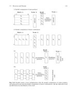
Figure 16.8 Distribution of maximum compressive stress, comparison with theory
16.4 DYNAMICS
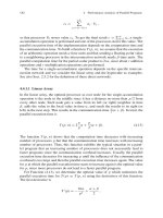
Here we extend the coupling method to dynamics. The dynamic equilibrium equations
which arise from finite element discretisation (see Bathe
4
) can be written as
(16.19)
where
>
@
M ,
>
@
C ,
>
@
K are the assembled mass, damping and stiffness matrices and
^
`
u

,
^
`
u

,
^`
u are the acceleration, velocity and displacement vectors. The time may be

discretised into n time steps of size
t' . Assuming an average acceleration within the
time step the system of differential equations can be transformed into a system of
algebraic equations (Newmark method
4
)
(16.20)
where
tnt 'and (1)tn t

'



A
nal
y
sis
min
V

Theory
>
@
^`
>
@
^`
>
@

^` ^`
 Mu Cu Ku F
 
^`
^`
()t
ªº

¬¼
Ku F
COUPLED BOUNDARY ELEMENT/FINITE ELEMENT ANALYSIS 447
The “dynamic stiffness matrix” is given by:
(16.21)

and
(16.22)

Since we have already worked out a “dynamic stiffness matrix” of the boundary element
region in Chapter 14 the coupling procedure is now straightforward. For a fully coupled
problem the system of equations is given by
(16.23)

16.4.1 Example
The example is that of a concrete column embedded in a semi-infinite soil mass. The
description of the problem can be seen in Figure 16.9. The top of the column is subjected
to a suddenly applied load p(t) of 1 MN/m
2
. The material properties for the column are:
spec. weight= 2500 kg/m
3

, E=30 000 MN/m
2
,
Q
=0.2. For the soil we have: spec.
weight= 2000 kg/m
3
, E=100 MN/m
2
,
Q
=0.2.

Figure 16.9 Description of example
Figure 16.10 shows the mesh used for the analysis it consists of a finite element region
that describes the column and a boundary element region that describes the semi-infinite
ground. The mesh has 1500 degrees of freedom. Figure 16.11 shows the time-dependent
>@ >@> @
2
42
t
t
ªº

¬¼
'
'
KMCK
^`
>@

^`^`^`
>@
^`^`^`
2
44
() () ()
2
() () ()
ttt
t
t
tt t
t

 
§·

¨¸
'
'
©¹
§·

¨¸
'
©¹
FM u u u
Cu u F





^`
^` ^`
()
BE FE
BE FE
t
ªº ªº
 
¬¼ ¬¼
NK K u F F
()
p
t
()
p
t
t
448 The Boundary Element Method with Programming
displacements at the top of the column obtained from the analysis. The results compare
well with a reference solution with the FEM that used 1 Million elements.
Figure 16.10 Coupled mesh
Figure 16.11 Displacement at the top of the column
16.5 CONCLUSION
In this chapter we have shown how the capability of a finite or boundary element
program can be easily extended so that the advantages of both methods can be combined
giving the user “the best of both worlds”. We have shown one example where the
capability of the BEM in dealing with infinite domains was exploited. Many other such
examples exist and we will show in the next chapter one industrial application that could

(seconds)
COUPLED BOUNDARY ELEMENT/FINITE ELEMENT ANALYSIS 449
not have been analysed with either method given the restrictions regarding time and
computing resources.
Although it is true that both methods can deal with almost any problem that arises in
engineering (and comprehensive text books on the FEM and BEM assert this), it is also
clear that they are more appropriate for some applications and less so for others. It
should have become clear to the reader, for example, that the BEM is well suited for
problems involving a small ratio of boundary surface to volume. Extreme cases of this
are problems which can be considered as involving an infinite volume. Such problems
exist, for example, in geomechanics
5
, where the earth’s crust has no lateral boundaries.
Another extreme where the ratio boundary surface to volume is very large is the
application to thin shell structures.
Another aspect is the importance that is given to surface stresses. As we have seen in
Chapter 9, stresses at the surface are computed more accurately with the BEM than with
the FEM. We have shown that problems where “body forces” occur in the domain, as for
example plasticity problems, etc., can be handled with the BEM but it has to be admitted
that implementation is much more involved than with the FEM. A final aspect which is
also gaining more importance, is the suitability of the methods for implementation with
regards to computer hardware. The future seems to lie in massive parallel processing and
we have seen in Chapter 8 that the BEM seems to lend itself to parallel programming.
16.6 REFERENCES

1. Zienkiewicz O.C. ,Kelly D.W. and Bettess P. (1979) Marriage a la mode- the best of
both worlds (finite elements and boundary integrals) Chapter 5 of Energy Methods in
Finite Element Analysis (ed. R.Glowinski, E.Y. Rodin and O.C.Zienkiewicz), pp. 82-
107, Wiley, London.
2. Beer G. (1977) Finite element, boundary element and coupled analysis of unbounded

problems in elastostatics. Int. J. Numer. Methods Eng., 11, 355-376
3. Beer G. (1998) Marriage a la mode (finite and boundary elements) revisited. In
Computational Mechanics New Trends and Applications (E.Onate and S.R.Idelsohn
(eds).
4. Bathe K.J. (1982) Finite Element procedures in engineering analysis. Prentice Hall.
5. Beer G., Golser H., Jedlitschka G. and Zacher P. Coupled finite element/boundary
element analysis in rock mechanics - industrial applications. Rock Mechanics for
Industry, Amadei, Kranz, Scott & Smeallie(eds). Balkema,Rotterdam. 133-140.

17
Industrial Applications
Grau ist alle Theorie
(Grey is all theory )
J.W. Goethe

17.1 INTRODUCTION
So far in this book we have developed software which can be applied to compute test
examples. The purpose of this was to enable the reader to become familiar with the
method, ascertain its accuracy and get a feel for the range of problems that can be
solved. The emphasis in software development has been on an implementation that was
concise and clear and could be well understood. As pointed out in the introduction to
programming, this is not necessarily the most efficient code in terms of storage and
computer resources.
If one wants to tackle real engineering problems one is inevitably faced with the need
to develop efficient code. The programs developed here would be unsuitable for such a
task. Aspects of the software that need to be improved are:
x Greater efficiency in the computation of coefficient matrices by rearranging DO
loops, so that calculations that are independent of the DO loop variable are taken
outside the loop.
x Greater efficiency in data and memory management so that data are only stored in

RAM when they are needed, use of hard disk storage to achieve this (see for
example [1] ).

It has been shown in Chapter 8 that a significant gain in efficiency can be achieved
by using element by element techniques and parallel programming. Indeed, to solve
452 The Boundary Element Method with Programming
problems at an industrial scale in a short time, special hardware, such as parallel
computers may have to be used.
In this chapter we attempt to show applications of the boundary element and coupled
methods which have been compiled from a number of tasks that have been carried out
over more than two decades using BEFE
2
, a combined finite element/boundary element
program. The purpose of the chapter is twofold. Firstly, an attempt is made to
demonstrate the applications for which the BEM may have a particular advantage over
the FEM. These applications include:
x Problems involving stress concentrations at the boundary, such as they occur in
mechanical engineering
x Problems consisting of infinite or semi-infinite domains, such as those occurring in
geotechnical engineering
x Problems involving slip and separation at material interfaces, such as they appear in
mechanical and geotechnical engineering
x Contact and crack propagation problems

The second purpose of this chapter is to show how the very complex problems that
invariably arise in industrial applications can be simplified, so that the analysis can be
performed in a reasonable short time.
It is very rarely the case that a problem can be modelled exactly as it is. In most cases
we have to decrease its complexity. The process of modelling a given complex structure
requires a lot of engineering ingenuity and experience. When we simplify a complex

problem we must ensure that the important influences are retained neglecting other less
important ones. For example, in a structural problem some parts of the structure may not
contribute significantly to its load carrying capacity but are there because of design
considerations.
One very significant modelling decision is if a 3-D analysis needs to be carried out.
Obviously this would result in much greater analysis effort. As an example in
geotechnical engineering consider a tunnel which is very long compared to its diameter.
If we are only interested in the displacements and stresses at a cross section far away
from the tunnel face, then a plane strain analysis would obviously suffice. Another way
of simplifying a problem is the introduction of planes of symmetry. As we have seen in
some of the examples in Chapter 10, this results in considerable savings. Obviously if
the prototype to be analysed is symmetric there is no loss in modelling accuracy. In
some cases, however, symmetry planes can be assumed without significant loss in
accuracy even if the prototype itself is not exactly symmetric.
In the following we will present background information on each application, in some
cases together with a story associated with it. We will start with the description of the
problem and how it was simplified. We show the boundary element mesh generated and
the results obtained. Comments are made on the quality of the results. The problem areas
are divided into mechanical, geotechnical, geotechnical civil engineering and reservoir
engineering.
INDUSTRIAL APPLICATIONS 453


17.2 MECHANICAL ENGINEERING
17.2.1 A cracked extrusion press causes concern
A small company in Austria manufactures rolled thin tubes by extrusion. The extrusion
press in use was 35 years old and made of cast iron (see Figure 17.1). During a routine
inspection cracks were detected on the surface of the cast iron casing, as indicated. The
company was in the process of ordering a new press, however delivery was expected to
take more than six months. There was some concern that something dramatic might

happen during the extrusion process with the press suddenly breaking, meaning not only
a danger to lives but also the possibility of losing the press. With full order books the
latter was a very serious economic threat.
Figure 17.1 35 year old drawing of extrusion press with location of cracks indicated
The aim of the analysis was therefore to determine:

x If the existing cracks would propagate
x If this propagation would lead to a sudden collapse of the structure

The geometry of the part to be analysed was fairly complicated and had to be
reconstructed from the original plans. For the purpose of the analysis it was assumed
that there were two planes of symmetry, as shown in Figure 17.2, although this was not
strictly true.
The cylindrical bar restraining the casing was not explicitly modelled but instead
appropriate Dirichlet boundary conditions were applied. Each time a tube is extruded the
casing is loaded with a force of 3700 tons (37 MN), as shown by the arrows. Although
Cracks
observed
454 The Boundary Element Method with Programming
this load is actually applied dynamically it was assumed to be static for the purpose of
the analysis.

Figure 17.2 Boundary element model showing axes of symmetry and holding bar
The drawing in Figure 17.2 actually looks like a finite element mesh but if viewed
from the symmetry planes (Fig. 17.3) one can notice that, in contrast to a FEM
discretisation, there are no elements inside the material. The mesh consists of a total of
1437 linear boundary elements and has 4520 degrees of freedom.
There were two reasons why a boundary element analysis was chosen for this
problem. Firstly, the generation of the mesh was found to be easier, since no internal
INDUSTRIAL APPLICATIONS 455

elements and connection between surfaces had to be considered. Secondly, the task was
to determine surface stresses and then to investigate crack propagation. As outlined
previously, the BEM is well suited for this type of analysis.

Figure 17.3 Boundary element mesh viewed from one of the symmetry planes
Initially, an analysis with only one region was carried out without considering the
presence of cracks. This was done in order to check that the analysis was able to predict
crack initiation. The criteria chosen for this was the maximum tensile strength of the
material, taking into consideration the dynamic nature of the loading and the number of
cycles that the press had so far sustained (approx. 2 million cycles). This analysis was
also carried out to see if the model was adequate and to enable the client to get
confidence in the BEM analysis proposed. The contours of maximum stress obtained
from the single region analysis, shown in Figure 17.4, clearly indicate a stress
concentration at the locations where cracks were observed, of a magnitude which would
cause crack initiation there after a number of cycles.
After this verification of the model, a multi-region analysis was carried out. For this
each of the flanges where the crack was observed was divided into two regions. For
simplicity it was assumed that the crack path was known a priori and is in the diagonal
direction, as observed. Along this assumed crack path an interface was assumed between
regions and the interface was allowed to slip and separate.
456 The Boundary Element Method with Programming
Figure 17.4 Contours of maximum principal stress

Figure 17.5 Displaced shape showing crack opening
INDUSTRIAL APPLICATIONS 457

It was found that in the worst case (lowest parameters assumed for the material) the
crack would tend to propagate to the corners of the flange (Figure 17.5). However, even
with the crack propagated that far the model predicted that there would be no dramatic
failure of the casing. Instead, the deformations would become so large that the press
would become inoperable.
After half a year the new press arrived and was installed. The old press gave service
without any major problems prior to replacement.
The advantages of the BEM over a FEM model may be summarised as:

x The fact that there are no elements inside and no connections were required between
elements on opposing boundaries the mesh generation was simplified. The number
of unknowns and elements was also reduced.
x The stress concentrations were computed more accurately because they are not
obtained using an extrapolation from inside the domain but from boundary results.
x The method was well suited to model crack propagation.
17.3 GEOTECHNICAL ENGINEERING
17.3.1 CERN Caverns
The European Laboratory for Particle Physics (CERN) is the world’s largest research
laboratory for subatomic particle physics. The laboratory occupies 602 hectars across the
Franco-Swiss border and includes a series of linear and circular particle accelerators.
The main Large Electron Positron (LEP) accelerator has a circumference of 26.7 km and
a series of underground structures situated at eight access and detector points (Fig. 17.6).
The LEP accelerator has been operating since 1989 but in 2000 it has been shut down
and replaced by the Large Hadron Collider (LHC) in 2005. This will use all existing
LEP structures but will also require new surface and underground works. Two new
detectors will be installed in two separated cavern systems, called Point 1 and 5.
Here we will present the three-dimensional analysis of the new caverns of Point 5
3,4

(Fig 17.7). This is an interesting application because point 1 of the LHC was analysed

using the finite element method and a picture of the results appear in the cover of the
book Programming the Finite Element Method
5
. According to a report published on this
study the mesh had approx 300 000 degrees of freedom and a supercomputer was
required to solve the problem.
Initially, an elastic analysis was carried out with the single region BE mesh shown in
Figure 17.8. The aim of the analysis was to ascertain the range of validity of 2-D
analyses carried out with a distinct element code.

458 The Boundary Element Method with Programming

Figure 17.6 Photo showing location of the CERN particle accelerator
Figure 17.7 Cavern system at Point 5, showing existing and new structures

INDUSTRIAL APPLICATIONS 459


Figure 17.8 Boundary element mesh, single region analysis


Figure 17.9 Results of single region analysis: contours of maximum compressive stress

Quadratic
boundary elements

“plane strain” infinite
boundary elements

460 The Boundary Element Method with Programming

The overburden above crown is about 75 m. In the analysis therefore the ground
surface was assumed to be sufficiently far away so that its influence on the cavern was
neglected. In order to reduce the number of unknowns “plane strain” infinite elements
were used, as introduced in section 3.7.2. and as indicated in Figure 17.8. The mesh has
a total of 4278 unknowns and the calculation took 10 minutes on a PC. The results of the
analysis are shown in Figure 17.9. Here the maximum compressive stress is plotted on
two planes inside the rock mass. Looking at the horizontal result plane it can be seen that
at a cross-section between the vertical shafts, nearly plane strain conditions are obtained,
warranting a 2-D analysis there.

Figure 17.10 Coupled boundary element / finite element mesh of USC55 cavern
Figure 17.11 Displacements of the concrete shell due to swelling

Infinite ‘plane
strain’ boundary
elements
Linear boundary
elements
Linear cells
Linear ‘brick’
finite elements
Symmetry plane
INDUSTRIAL APPLICATIONS 461



Geologists found that a portion of the soil above the cavern could swell significantly
if subjected to moisture. Therefore, an analysis had to be carried out to determine the
effect of swelling on the final concrete lining. Obviously, this cannot be simplified as a
2-D problem because the concrete lining acts as a 3-D shell structure. For this analysis a

coupled finite element/boundary element analysis was performed with the thin concrete
shell modelled by finite elements. The swelling zone was modelled by linear cells as
explained in Chapter 13. In addition a symmetry plane was assumed between the large
and the small cavern. Even though in reality no symmetry exists this was thought to be
acceptable since the assumption that the second cavern is the same size as the first one
would give results that are on the safe side. The main reason for the choice of this mesh
was that due to time limitations the job had to be completed quickly and only standard
PCs were available for performing the analysis. The coupled mesh of cavern USC 55 is
shown in Figure 17.10. The mesh has a total of 7575 degrees of freedom and the run
took 45 minutes on a standard PC. Most of the computing time was for computation of
the stiffness matrix of the boundary element region
The displacements of the concrete lining due to swelling were determined from the
analysis. These are shown in figure 17.11. From these displacements the internal forces
in the shell (bending moment and normal force) could be determined and used for
designing the reinforcement. The analysis shown here demonstrates that with limited
resources available (time and computer), boundary element and coupled analysis offer
an efficient alternative to the FEM.
17.4 GEOLOGICAL ENGINEERING
17.4.1 How to find gold with boundary elements
The analysis was performed to test a theory of geologists that gold dust was originally
suspended in water and was deposited in the ground in locations that had a significantly
smaller amount of compressive stress than the surrounding rock
6
. This seems to make
sense, since deposits would naturally occur in voids, i.e., areas where the compressive
stress is zero.
Since Australia is one of the richer countries in terms of gold resources the story
takes place there. In particular, the analysis concentrates on what is presumed to have
occurred in a region of Western Australia (where a deposit was found) during the
Precambrian period (about 800 million years ago). The geologists assume that the region

was shortened in an approximate east/west direction and that the deposit was formed at
approximately 2.5 km of depth below the surface. On this basis it was suggested that a
volume of rock of about 2000x2000x1000 m dimension with the geological structure as
observed in that area should be analysed. The geological structures are shown in Figures
17.12 and 17.13. Figure 17.12 shows contours of the contact between different rock
types, whereas Fig.17.13 shows contours of two faults (termed Lucky and Golden
faults).
462 The Boundary Element Method with Programming


Figure 17.12 Contours of contact between different rock types
Figure 17.13 Contours of Lucky and Golden faults
It was assumed that the block to be analysed was subjected to 2000 m of overburden
(which was subsequently eroded) and to tectonic stresses which were estimated from the
presumed shortening of the region.
INDUSTRIAL APPLICATIONS 463


Figure 17.14 Definition of boundary element regions

Figure 17.15 Block analysed showing stress boundary conditions applied
132
MPa
50
MPa
145
MPa

Region I
Region II

Region III
Region IV
464 The Boundary Element Method with Programming
Figure 17.16 Contours of maximum compressive principal stress
For the analysis a multi-region boundary element method was used with special
contact/joint algorithms implemented on the interfaces between regions. Figure 17.14
shows a view of the four regions considered. Figure 17.15 shows the block analysed
with stress boundary conditions applied. In this figure the deformation of the blocks and
the movements on the Golden and Lucky faults can be seen. The results of the analysis
can be seen in Figure 17.16 as contours of the maximum (compressive) principal stress
on the contact between regions I and II. One can clearly see an anomaly of the
compressive stress (“hot spot”) and this is near the location where the gold deposit was
assumed to be. So the boundary element method was successfully applied to find gold
deposits. Note that an analysis with a domain type method would be feasible. However,
the mesh generation would be more complicated because of the presence of elements
inside the regions and the necessity to assure proper connectivity.
17.5 CIVIL ENGINEERING
17.5.1 Masjed-o-Soleiman underground power house
The Masjed-o-Soleiman hydroelectric scheme is situated in the south of Iran. The
powerhouse is situated underground. In 2002 the last of 4 turbines were installed in the
existing powerhouse and an extension of the facility to house another 4 turbines was
underway. During the excavation of the extension, cracks were observed in the concrete
walls of the existing powerhouse, which caused some concern. In addition
„hot spot“
INDUSTRIAL APPLICATIONS 465


measurements from pressure cells installed behind the concrete walls recorded
seasonally dependent pressure increases that showed an increasing tendency. Following
a visit by the panel of experts it was decided to carry out a numerical analysis. The aim

of the analysis was to determine the cause of the cracks and to predict if the cracking
would get worse because of continuing excavation activity on the extension.
Figure 17.17 View of hydroelectric plant, the powerhouse cavern is inside the mountain on the
left of the dam

Figure 17.18 Layout of the Caverns indicating existing caverns and caverns being excavated
466 The Boundary Element Method with Programming
Figure 17.17 shows a view of the hydroelectric facility and Figure 17.18 a plan of the
layout showing the existing powerhouse cavern and the extension under construction.
The areas where cracking was observed are shown in Figure 17.19. Special
consideration was given to the circled area near the construction of the extension.
Figure 17.19 Plan of powerhouse depicting areas where cracks were observed
The ground conditions in the vicinity of the caverns, as shown in Figure 17.20, are
dominated by layers of very weak mudstone and sandstone.
Figure 17.20 Geological conditions near the caverns
INDUSTRIAL APPLICATIONS 467


To ascertain the fineness of the mesh required for the analysis and the displacement
patterns, a 3-D Boundary Element analysis was first carried out.
Figure 17.21 Boundary element mesh of caverns and computed deformations
Figure 17.22 Coupled mesh for the analysis of powerhouse cavern and concrete powerhouse
structure
468 The Boundary Element Method with Programming
However, this analysis does not consider the presence of geological features and non-
linear effects, which are important. Figure 17.21 shows the mesh with quadratic (8-node)
boundary elements and the result for the case where both caverns are excavated, plotted
as displacement contours on the excavation surface. It can be seen that for a large
portion of the cavern plane strain conditions can be observed. It was therefore decided
that the mesh could be reduced by the use of infinite plane strain boundary elements as

they have been introduced in Chapter 3.
For a meaningful analysis, however, the effect of the geological features as well as
the non-linear behaviour of the ground had to be considered. For this purpose a coupled
finite element/boundary element mesh was constructed as shown in Figure 17.22. Here
the rock mass in the vicinity of the cavern, as well as the concrete structure of the
powerhouse is discretised into finite elements. Plane strain boundary elements were used
to shorten the mesh in the direction along the cavern, taking into consideration the
displacement conditions, as depicted in Figure 17.21. This analysis allows to consider
the geological features as well as the nonlinear behaviour of the ground (in particular the
mudstone layers).
Figure 17.23 Two of the stages considered in the analysis
Several excavation stages were considered and two of these are shown in Figure
17.23. The mesh on the left models the complete excavation of cavern 1, the one on the
right the construction of the powerhouse structure and the excavation stage of the
extension as existed during the visit of the panel of experts. Figure 17.24 shows the
displaced shape on a section through the end of the existing cavern near the extension
excavation. The deformation of the FEM-BEM interface can be seen especially on top of
the cavern, so an analysis without coupling to BEM would not have yielded meaningful
Existing powerhouse cavern
excavate
d
Powerhouse structure
installed, excavation of
extension
,
status Nov. 2003
INDUSTRIAL APPLICATIONS 469


results. A view of the finite element mesh of the powerhouse structure, indicating the

location of the cracks near the extension is shown in Figure 17.25.


Figure 17.24 Displaced shape in a cross-section through the end of the powerhouse.

Figure 17.25 View showing the concrete powerhouse and the location of the cracks
470 The Boundary Element Method with Programming
Figure 17.26 shows one result of the analysis namely the stress distribution in the
concrete wall plotted as principal stress vectors. It can be seen that the observed crack
pattern on the right is perpendicular to the maximum computed principal stress.

Figure 17.26 Predicted stress pattern in wall and crack pattern observed.
This is a nice example of the use of a coupled analysis because it substantially reduces
the effort. Without coupling to BEM the mesh would have to be made much larger, to
reduce the effect of artificial boundary conditions to an acceptable level. It should be
noted here that with the methods for non-linear analysis described in Chapter 15 and for
dealing with heterogeneous ground conditions outlined in Chapter 18 it would have been
possible to completely avoid the discretisation into finite elements of the ground
surrounding the cavern. All that would be required is to subdivide the ground into cells.
However, at the time of the analysis these capabilities were not available.
17.6 RESERVOIR ENGINEERING
17.6.1 Borehole stability
The example relates to some work performed in cooperation with the University of
Kuwait. For oil recovery vertical boreholes are drilled to a depth of several thousand
meters. In order recover as much oil as possible from one bore hole, deviated boreholes
are drilled as shown in Figure 17.27. The angle of deviation of the lateral bore varies
from 30° to 60° and the direction of the deviation with respect to the virgin stress field
also varies. Since the boreholes are drilled in a highly pre-stressed rock mass, mud
pressure has to be applied in order to stabilize the borehole. The questions to be
INDUSTRIAL APPLICATIONS 471

answered by the simulation were with respect to the stability of the rock near the
junction of the vertical and the deviated borehole.
Figure 17.27 Sketch of borehole junction
To determine the areas in the rock mass that are likely to break an elastic analysis
was performed. The result of the analysis was a contour plot of a yield function,
()F
V
.
The yield functions used were the Mohr-Coulomb and Hoek and Brown models. The
mesh used for the analysis for a 45° deviation is plotted in Figure 17.28 on the left.
Figure 17.28 Boundary element mesh (left) and results of the analysis (right) plotted on surface
and dummy plane