Advanced Methods and Tools for ECG Data Analysis - Part 6 docx
Bạn đang xem bản rút gọn của tài liệu. Xem và tải ngay bản đầy đủ của tài liệu tại đây (1002 KB, 40 trang )
P1: Shashi
August 24, 2006 11:46 Chan-Horizon Azuaje˙Book
6.4 Empirical Nonlinear Filtering 185
Figure 6.4 Illustration of NNR: (a) original noisy ECG signal, y(t); (b) underlying noise-free ECG,
x(t); (c) noise-reduced ECG signal, z(t); and (d) remaining error, z(t)−x(t). The signal-to-noise ratio
was γ = 10 and the NNR used parameters m = 20, d = 1, and r = 0.08.
factor, χ, and the correlation, ρ, as a function of the reconstruction dimension, m,
for signals having γ = 10, 5, 2.5. For γ = 10, maxima occur at χ = 2.2171 and
ρ = 0.9990, both with m = 20. For the intermediate signal to noise ratio, γ = 5,
maxima occur at χ = 2.6605 and ρ = 0.9972 with m = 20. In the case of γ = 2.5,
the noise reduction factor has a maximum, χ = 3.3996 at m = 100, whereas the
correlation, ρ = 0.9939, has a maximum at m = 68.
ICA gave best results for all signal to noise ratios for a delay of d = 1. As may be
seen from Figure 6.5, optimizing the noise reduction factor, χ , or the correlation, ρ,
gave maxima at different values of m. For γ = 10, the maxima were χ = 26.7265
at m = 7 and ρ = 0.9980 at m = 9. For the intermediate signal to noise ratio,
γ = 5, the maxima are χ = 18.9325 at m = 7 and ρ = 0.9942 at m = 9. Finally
for γ = 2.5, the maxima are χ = 10.8842 at m = 8 and ρ = 0.9845 at m = 11. A
demonstration of the effect of optimizing the ICA algorithm over either χ or ρ is
illustrated in Figure 6.6. While both the χ-optimized cleaned signal [Figure 6.6(b)]
and the ρ-optimized cleaned signal [Figure 6.6(d)] are similar to the original noise-
free signal [Figure 6.6(a)], an inspection of their respective errors, [Figure 6.6(c)]
and [Figure 6.6(e)], emphasizes their differences. The χ-optimized outperforms the
ρ-optimized in recovering the R peaks.
A summary of the results obtained using both the NNR and ICA techniques
are presented in Table 6.1. These results demonstrate that NNR performs better in
terms of providing a cleaned signal which is maximally correlated with the original
P1: Shashi
August 24, 2006 11:46 Chan-Horizon Azuaje˙Book
186 Nonlinear Filtering Techniques
Figure 6.5 Variation in (a) noise reduction factor, χ , and (b) correlation, ρ, for ICA with recon-
struction dimension, m, and delay, d = 1. The signal-to-noise ratios are γ = 10 (•), γ = 5(
), and
γ = 2.5(
).
Table 6.1 Noise Reduction Performance in Terms of Noise
Reduction Factor, χ, and Correlation, ρ, for Both NNR and
ICA for Three Signal-to-Noise Ratios, γ = 10,5,2.5
Method Measure γ = 10 γ = 5 γ = 2.5
NNR χ 2.2171 2.6605 3.3996
ICA χ 26.7265 18.9325 10.8842
NNR ρ 0.9990 0.9972 0.9939
ICA ρ 0.9980 0.9942 0.9845
noise-free signal, whereas ICA performs better in terms of yielding a cleaned signal
which is closer to the original noise-free signal, as measured by an RMS metric.
The decision between seeking an optimal χ or ρ depends on the actual appli-
cation of the ECG signal. If the morphology of the ECG is of importance and the
various waves (P, QRS, T) are to be detected, then perhaps a large value of ρ is of
greater relevance. In contrast, if the ECG is to be used to derive RR intervals for
generating an RR tachogram, then the location in time of the R peaks are required.
In this latter case, the noise reduction factor, χ, is preferable since it penalizes heav-
ily for large squared deviations and therefore will favor more accurate recovery of
extrema such as the R peak.
6.5 Model-Based Filtering
The majority of the filtering techniques presented so far involve little or no assump-
tions about the nature of either the underlying dynamics that generated the signal
or the noise that masks it. These techniques generally proceed by attempting to
P1: Shashi
August 24, 2006 11:46 Chan-Horizon Azuaje˙Book
6.5 Model-Based Filtering 187
Figure 6.6 Demonstration of ICA noise reduction for γ = 10: (a) original noise-free ECG signal, x(t);
(b) χ-optimized noise-reduced signal, z
1
(t), with m = 7; (c) error, e
1
(t) = z
1
(t)−x(t); (d) ρ-optimized
noise-reduced signal, z
2
(t), with m = 8; and (e) error, e
2
(t) = z
2
(t)−x(t).
separate the signal and noise using the statistics of the data and often rely on a set
of assumed heuristics; there is no explicit modeling of any of the underlying sources.
If, however, a known model of the signal (or noise) can be built into the filtering
scheme, then it is likely that a more effective filter can be constructed.
The simplest model-based filtering is based upon the concept of Wiener filtering,
presented in Section 3.1. An extension of this approach is to use a more realistic
P1: Shashi
August 24, 2006 11:46 Chan-Horizon Azuaje˙Book
188 Nonlinear Filtering Techniques
model for the dynamics of the ECG signal that can track changes over time. The
advantage of such an approach is that once a model has been fitted to a segment of
ECG, not only can it produce a filtered version of the waveform, but the parameters
can also be used to derive wave onsets and offsets, compress the ECG, or classify
beats. Furthermore, the quality of the fit can be used to obtain a confidence measure
with respect to the filtering methods.
Existing techniques for filtering and segmenting ECGs are limited by the lack of
an explicit patient-specific model to help isolate the required signal from contam-
inants. Only a vague knowledge of the frequency band of interest and almost no
information concerning the morphology of an ECG are generally used. Previously
proposed adaptive filters [57, 58] require another reference signal or some ad hoc
generic model of the signal as an input.
6.5.1 Nonlinear Model Parameter Estimation
By employing a dynamical model of a realistic ECG, known as ECGSYN (described
in detail in Section 4.3.2), a tailor-made approach for filtering ECG signals is now
described.
The model parameters that are fit basically constitute a nondynamic version of
the model described in [6, 59] and add an extra parameter for each asymmetric
wave (only the T wave in the example given here). Each symmetrical feature of the
ECG (P,Q,R, and S) is described by three parameters incorporating a Gaussian
(amplitude a
i
, width b
i
) and the phase θ
i
= 2π/t
i
(or relative position with respect
to the R peak). Since the T wave is often asymmetric, it is described by the sum of
two Gaussians (and hence requires six parameters) and is denoted by a superscripted
− or + to indicate that they are located at values of θ (or t) slightly to either side of
the peak of the T wave (the original θ
T
that would be used for a symmetric model).
The vertical displacement of the ECG, z, from the isoelectric line (at an assumed
value of z = 0) is then described by an ordinary differential equation,
˙z(a
i
,b
i
,θ
i
) =−
i∈{P,Q, R,S,T
−
,T
+
}
a
i
θ
i
exp
−θ
2
i
2b
2
i
(6.25)
where θ
i
= (θ −θ
i
)mod(2π) is the relative phase. Numerical integration of (6.25)
using an appropriate set of parameter values, a
i
, b
i
, and θ
i
, leads to the familiar
ECG waveform.
One efficient method of fitting the ECG model described above to an observed
segment of the signal s(t) is to minimize the squared error between s(t) and z(t).
This can be achieved using an 18-dimensional nonlinear gradient descent in the
parameter space [60]. Such a procedure has been implemented using two different
libraries, the Gnu Scientific Libraries (GSL) in C, and in Matlab using the function
lsqnonlin.m.
To minimize the search space for fitting the parameters, (a
i
, b
i
, and θ
i
), a sim-
ple peak-detection and time-aligned averaging technique is performed to form an
average beat morphology using at least the first 60 beats centred on their R peaks.
The template window length is unimportant, as long as it contains all the PQRST
features and does not extend into the next beat. This method, including outlier
P1: Shashi
August 24, 2006 11:46 Chan-Horizon Azuaje˙Book
6.5 Model-Based Filtering 189
Figure 6.7 Original ECG, nonlinear model fit, and residual error.
rejection, is detailed in [61]. T
−
and T
+
are initialized ±40 ms either side of θ
T
.By
measuring the heights, widths, and positions of each peak (or trough), good initial
estimates of the model parameters can be made. Figure 6.7 illustrates an example
of a template ECG, the resulting model fit, and the residual error.
Note that it is important that the salient features that one might wish to fit
(the P wave and QRS segment in the case of the ECG) are sampled at a high
enough frequency to allow them to contribute sufficiently to the optimization. In
empirical tests it was found that when F
s
< 450 Hz, upsampling is required (using
an appropriate antialiasing filter). With F
s
< 450 Hz there are often fewer than 30
sample points in the QRS complex and this can lead to some unrealistic fits that
still fulfill the optimization criteria.
One obvious application of this model-fitting procedure is the segmentation
of ECG signals and feature location. The model parameters explicitly describe the
location, height, and width of each point (θ
i
, a
i
, and b
i
) in the ECG waveform,
in terms of a well-known mathematical object, a Gaussian. Therefore, the feature
locations and parameters derived from these (such as the P, Q, and T onset and hence
the PR and QT interval) are easily extracted. Onsets and offsets are conventionally
difficult to locate in the ECG, but using a Gaussian descriptor, it is trivial to locate
these points as two or three standard deviations of b
i
from the θ
i
in question.
Similarly, for ECG features that do not explicitly involve the P, Q, R, S,orT
points (such as the ST segment), the filtering aspect of this method can be applied.
P1: Shashi
August 24, 2006 11:46 Chan-Horizon Azuaje˙Book
190 Nonlinear Filtering Techniques
Furthermore, the error in the fitting procedure can be used to provide a confidence
measure for the estimates of any parameters extracted from the ECG signal.
A related application domain for this model-based approach is (lossy) com-
pression with a rate of (F
s
/3k : 1) per beat, where k = n + 2m is the number of
features or turning points used to fit the heartbeat morphology (with n symmetric
and m asymmetric turning points). For a low F
s
(≈ 128 Hz), this translates into a
compression ratio greater than 7:1 at a heart rate of 60 bpm. However, for high
sampling rates (F
s
= 1, 024) this can lead to compression rates of almost 60:1.
Although classification of each beat in terms of the values of a
i
, b
i
, and θ
i
is
another obvious application for this model, it is still unclear if the clustering of
the parameters is sufficiently tight, given the sympathovagal and heart-rate induced
changes typically observed in an ECG. It may be necessary to normalize for heart-
rate dependent morphology changes at least. This could be achieved by utilizing the
heart rate modulated compression factor α, which was introduced in [59]. However,
clustering for beat typing is dependent on population morphology averages for a
specific lead configuration. Not only would different configurations lead to different
clusters in the 18-dimensional parameter space, but small differences in the exact
lead placement relative to the heart would cause an offset in the cluster. A method
for determining just how far from the standard position the recording is, and a
transformation to project back onto the correct position would be required. One
possibility could be to use a procedure designed by Moody and Mark [62] for their
ECG classifier Aristotle. In this approach, the beat clusters are defined in a space
resulting from a Karhunen-Lo
`
eve (KL) decomposition and therefore an estimate of
the difference between the classified KL-space and the observed KL-space is made.
Classification is then made after transforming from the observation to classification
space in which the training was performed. By measuring the distance between the
fitted parameters and pretrained clusters in the 18-dimensional parameter space,
classification is possible. It should be noted that, as with all classifiers, if an artifact
closely resembles a known beat, a good fit to the known beat will obviously arise.
For this reason, setting tolerances on the acceptable error magnitude may be crucial
and testing on a set of labeled databases is required.
By fitting (6.25) to small segments of the ECG around each QRS-detection fidu-
cial point, an idealistic (zero-noise) representation of each beat’s morphology may be
derived. This leads to a method for filtering and segmenting the ECG and therefore
accurately extracting clinical parameters even with a relatively high degree of noise
in the signal. It should be noted that since the model is a compact representation of
oscillatory signals with few turning points compared to the sampling frequency and
it therefore has a bandpass filtering effect leading to a lossy transformation of the
data into a set of integrable Gaussians distributed over time. This approach could
therefore be used on any band-limited waveform. Moreover, the error in each fit can
provide beat-by-beat confidence levels for any parameters extracted from the ECG
and each fit can run in real time (0.1 second per beat on a 3-GHz P4 processor).
The real test of the filtering properties is not the residual error, but how distorted
the clinical parameters of the ECG are in each fit. In Section 3.1, an analysis of the
sensitivity of clinical parameters to the color of additive noise and the SNR is given
together with an independent method for calculating the noise color and SNR. An
online estimate of the error in each derived fit can therefore be made. By titrating
P1: Shashi
August 24, 2006 11:46 Chan-Horizon Azuaje˙Book
6.5 Model-Based Filtering 191
colored noise into real ECGs, it has been shown that errors in clinical parameters
derived from the model-fit method presented here are clinically insignificant in the
presence of high amounts of colored noise. However, clinical features that include
low-amplitude features such as the P wave and the ST level are more sensitive to
noise power and color. Future research will concentrate on methods to constrain
the fit for particular applications where performance is substandard.
An advantage of this method is that it leads to a high degree of compression and
may allow classification in the same manner as in the use of KL basis functions (see
Chapter 9). Although the KL basis functions offer a similar degree of compression
to the Gaussian-based method, the latter approach has the distinct advantage of
having a direct clinical interpretation of the basis functions in terms of feature
location, width, and amplitude. Using a Gaussian representation, onsets and offsets
of waves are easily located in terms of the number of standard deviations of the
Gaussian away from the peak of the wave.
6.5.2 State Space Model-Based Filtering
The extended Kalman filter (EKF) is an extension of the traditional Kalman filter
that can be applied to a nonlinear model [63, 64]. In the EKF, the full nonlinear
model is employed to evolve the states over time while the Kalman filter gain and the
covariance matrix are calculated from the linearized equations of motion. Recently,
Sameni et al. [65] used an EKF to filter noisy ECG signals using the realistic artificial
ECG model, ECGSYN described earlier in Section 2.2. The equations of motion
were first transformed into polar coordinates:
˙r = r(1 −r)
˙
θ = ω (6.26)
˙z =−
i
a
i
θ
i
exp
−
θ
2
i
2b
2
i
− (z − z
0
)
Using this representation, the phase, θ, is given as an explicit state variable and r
is no longer a function of any of the other parameters and can be discarded. Using
a time step of size δt, the two-dimensional equations of motion of the system, with
discrete time evolution denoted by n, may be written as
θ(n + 1) = θ(n) + ωδt
z(n + 1) = z(n) −
i
δta
i
θ
i
exp
−
θ
2
i
2b
2
i
+ ηδ t
(6.27)
where θ
i
= (θ −θ
i
)mod(2π) and η is a random additive noise. Note that η replaces
the previous baseline wander term and describes all the additive sources of process
noise.
In order to employ the EKF, the nonlinear equations of motion must first be
linearized. Following [65], one approach is to consider θ and z as the underlying
state variables and the model parameters, a
i
, b
i
, θ
i
, ω, η as process noises. Putting
all these together gives a process noise vector,
w
n
= [a
P
, , a
T
, b
P
, , b
T
, θ
P
, , θ
T
, ω, η]
†
(6.28)
P1: Shashi
August 24, 2006 11:46 Chan-Horizon Azuaje˙Book
192 Nonlinear Filtering Techniques
with covariance matrix Q
n
= E{w
n
w
n
†
} where the subscript † denotes the trans-
pose.
The phase of the observations ψ
n
, and the noisy ECG measurements s
n
are
related to the state vector by
ψ
n
s
n
=
10
01
θ
n
z
n
+
ν
(1)
n
ν
(2)
n
(6.29)
where ν
n
= [ν
(1)
n
, ν
(2)
n
]
†
is the vector of measurement noises with covariance matrix
R
n
= E{ν
n
ν
n
†
}.
The variance of the observation noise in (6.29) represents the degree of un-
certainty associated with a single observation. When R
n
is high, the EKF tends to
ignore the observation and rely on the underlying model dynamics for its output.
When R
n
is low, the EKF’s gain adapts to incorporate the current observations.
Since the 17 noise parameters in (6.28) are assumed to be independent, Q
k
and R
n
are diagonal. The process noise η is a measure of the accuracy of the model, and is
assumed to be a zero-mean Gaussian noise process.
Using this EKF formulation, Sameni et al. [65] successfully filtered a series
of ECG signals with additive Gaussian noise. An example of this can be seen in
Figure 6.8. Future developments of this model are therefore very promising, since the
Figure 6.8 Filtering of noisy ECG using EKF: (a) original signal; (b) noisy signal; and (c) denoised
signal.
P1: Shashi
August 24, 2006 11:46 Chan-Horizon Azuaje˙Book
6.6 Conclusion 193
combination of a realistic model and a robust tracking mechanism make the concept
of online signal tracking in real time feasible. A combination of an initialization
with the nonlinear gradient descent method from Section 6.5.1 to determine initial
model parameters and noise estimates, together with subsequent online tracking,
may lead to an optimal ECG filter (for normal morphologies). Furthermore, the
ability to relate the parameters of the model to each PQRST morphology may lead
to fast and accurate online segmentation procedures.
6.6 Conclusion
This chapter has provided a summary of the mathematics involved in reconstructing
a state space using a recorded signal so as to apply techniques based on the theory of
nonlinear dynamics. Within this framework, nonlinear statistics such as Lyapunov
exponents, correlation dimension, and entropy were described. The importance of
comparing results with simple benchmarks, carrying out statistical tests and using
confidence intervals when conveying estimates was also discussed. This is important
when employing nonlinear dynamics as the basis of any new biomedical diagnostic
tool.
An artificial electrocardiogram signal, ECGSYN, with controlled temporal and
spectral characteristics was employed to illustrate and compare the noise reduc-
tion performance of two techniques, nonlinear noise reduction and independent
components analysis. Stochastic noise was used to create data sets with different
signal-to-noise ratios. The accuracy of the two techniques for removing noise from
the ECG signals was compared as a function of signal-to-noise ratio. The quality of
the noise removal was evaluated by two techniques: (1) a noise reduction factor and
(2) a measure of the correlation between the cleaned signal and the original noise-
free signal. NNR was found to give better results when measured by correlation. In
contrast, ICA outperformed NNR when compared using the noise reduction factor.
These results suggest that NNR is superior at recovering the morphology of the
ECG and is less likely to distort the shape of the P, QRS, and T waves, whereas
ICA is better at recovering specific points on the ECG such as the R peak, which is
necessary for obtaining RR intervals.
Two model-based filtering approaches were also introduced. These methods use
the dynamical model underlying ECGSYN to provide constraints on the filtered sig-
nal. A nonlinear least squares parameter estimation procedure was used to estimate
all 18 parameters required to specify the morphology of the ECG waveform. In
addition, an approach using the extended Kalman filter applied to a discrete two-
dimensional adaptation of ECGSYN in polar coordinates was also employed to
filter an ECG signal.
The correct choice of filtering technique depends not only on the character-
istics of the noise and signal in the time and frequency domains, but also on the
application. It is important to test a candidate filtering technique over a range of
possible signals (with a range of signal to noise ratios and different noise pro-
cesses) to determine the filter’s effect on the clinical parameter or attribute of
interest.
P1: Shashi
August 24, 2006 11:46 Chan-Horizon Azuaje˙Book
194 Nonlinear Filtering Techniques
References
[1] Papoulis, P., Probability, Random Variables, and Stochastic Processes, 3rd ed., New York:
McGraw-Hill, 1991.
[2] Schreiber, T., and D. T. Kaplan, “Nonlinear Noise Reduction for Electrocardiograms,”
Chaos, Vol. 6, No. 1, 1996, pp. 87–92.
[3] Cardoso, J. F., “Multidimensional Independent Component Analysis,” Proc. ICASSP’98,
Seattle, WA, 1998.
[4] Clifford, G. D., and P. E. McSharry, “Method to Filter ECGs and Evaluate Clinical Param-
eter Distortion Using Realistic ECG Model Parameter Fitting,” Computers in Cardiology,
September 2005.
[5] Moody, G. B., and R. G. Mark, “Physiobank: Physiologic Signal Archives for Biomedical
Research,” MIT, Cambridge, MA, updated June
2006.
[6] McSharry, P. E., et al., “A Dynamical Model for Generating Synthetic Electrocardiogram
Signals,” IEEE Trans. Biomed. Eng., Vol. 50, No. 3, 2003, pp. 289–294.
[7] Kantz, H., and T. Schreiber, Nonlinear Time Series Analysis, Cambridge, U.K.: Cambridge
University Press, 1997.
[8] McSharry, P. E., and L. A. Smith, “Better Nonlinear Models from Noisy Data: Attractors
with Maximum Likelihood,” Phys. Rev. Lett., Vol. 83, No. 21, 1999, pp. 4285–4288.
[9] McSharry, P. E., and L. A. Smith, “Consistent Nonlinear Dynamics: Identifying Model
Inadequacy,” Physica D, Vol. 192, 2004, pp. 1–22.
[10] Packard, N., et al., “Geometry from a Time Series,” Phys. Rev. Lett., Vol. 45, 1980, pp.
712–716.
[11] Takens, F., “Detecting Strange Attractors in Fluid Turbulence,” in D. Rand and L. S.
Young, (eds.), Dynamical Systems and Turbulence, New York: Springer-Verlag, Vol. 898,
1981, p. 366.
[12] Broomhead, D. S., and G. P. King, “Extracting Qualitative Dynamics from Experimental
Data,” Physica D, Vol. 20, 1986, pp. 217–236.
[13] Sauer, T., J. A. Yorke, and M. Casdagli, “Embedology,” J. Stats. Phys., Vol. 65, 1991,
pp. 579–616.
[14] Fraser, A. M., and H. L. Swinney, “Independent Coordinates for Strange Attractors from
Mutual Information,” Phys. Rev. A, Vol. 33, 1986, pp. 1134–1140.
[15] Rosenstein, M. T., J. J. Collins, and C. J. De Luca, “Reconstruction Expansion as a
Geometry-Based Framework for Choosing Proper Time Delays,” Physica D, Vol. 73,
1994, pp. 82–98.
[16] Kennel, M. B., R. Brown, and H. D. I. Abarbanel, “Determining Embedding Dimension
for the Phase-Space Reconstruction Using a Geometrical Construction,” Phys. Rev. A,
Vol. 45, No. 6, 1992, pp. 3403–3411.
[17] Strang, G., Linear Algebra and Its Applications, San Diego, CA: Harcourt College Pub-
lishers, 1988.
[18] Lorenz, E. N., “A Study of the Predictability of a 28-Variable Atmospheric Model,” Tellus,
Vol. 17, 1965, pp. 321–333.
[19] Abarbanel, H. D. I., R. Brown, and M. B. Kennel, “Local Lyapunov Exponents Computed
from Observed Data,” Journal of Nonlinear Science, Vol. 2, No. 3, 1992, pp. 343–365.
[20] Glass, L., and M. Mackey, From Clocks to Chaos: The Rhythms of Life, Princeton, NJ:
Princeton University Press, 1988.
[21] Wolf, A., et al., “Determining Lyapunov Exponents from a Time Series,” Physica D, Vol.
16, 1985, pp. 285–317.
[22] Sano, M., and Y. Sawada, “Measurement of the Lyapunov Spectrum from a Chaotic Time
Series,” Phys. Rev. Lett., Vol. 55, 1985, pp. 1082–1085.
P1: Shashi
August 24, 2006 11:46 Chan-Horizon Azuaje˙Book
6.6 Conclusion 195
[23] Eckmann, J. P., et al., “Liapunov Exponents from Time Series,” Phys. Rev. A, Vol. 34,
No. 6, 1986, pp. 4971–4979.
[24] Brown, R., P. Bryant, and H. D. I. Abarbanel, “Computing the Lyapunov Spectrum of a
Dynamical System from an Observed Time Series,” Phys. Rev. A, Vol. 43, No. 6, 1991,
pp. 2787–2806.
[25] McSharry, P. E., “The Danger of Wishing for Chaos,” Nonlinear Dynamics, Psychology,
and Life Sciences, Vol. 9, No. 4, October 2005, pp. 375–398.
[26] Rosenstein, M.T., J. J. Collins, and C.J. De Luca, “A Practical Method for Calculating
Largest Lyapunov Exponents from Small Data Sets,” Physica D, Vol. 65, 1994, pp. 117–
134.
[27] Kantz, H., “Quantifying the Closeness of Fractal Measures,” Phys. Rev. E, Vol. 49, No.
6, 1994, pp. 5091–5097.
[28] Hegger, R., H. Kantz, and T. Schreiber, “TISEAN: Nonlinear Time Analysis
Software,” Max-Planck-Institut f
¨
ur Physik Komplexer System, pks-
dresden.mpg.de/
∼
tisean/, December 2005.
[29] Renyi, A., Probability Theory, Amsterdam: North Holland, 1971.
[30] Ott, E., T. Sauer, and J. A. Yorke, Coping with Chaos, New York: John Wiley & Sons,
1994.
[31] Grassberger, P., and I. Procaccia, “Characterization of Strange Attractors,” Phys. Rev.
Lett., Vol. 50, 1983, pp. 346–349
[32] Theiler, J. T., “Spurious Dimension from Correlation Algorithms Applied to Limited Time-
Series Data,” Phys. Rev. A, Vol. 34, 1986, pp. 2427–2432.
[33] Provenzale, A., et al., “Distinguishing Between Low-Dimensional Dynamics and Random-
ness in Measured Time Series,” Physica D, Vol. 58, 1992, pp. 31–49.
[34] Takens, F., “On the Numerical Determination of the Dimension of an Attractor,”
in B. L. J. Braaksma, H. W. Broer, and F. Takens, (eds.), Dynamical Systems and
Bifurcations, Volume 1125 of Lecture Notes in Mathematics, Berlin, Germany: Springer,
1985, pp. 99–106.
[35] Guerrero, A., and L. A. Smith, “Towards Coherent Estimation of Correlation Dimension,”
Phys. Lett. A, Vol. 318, 2003, pp. 373–379.
[36] Ruelle, D., “Deterministic Chaos: The Science and the Fiction,” Proc. R. Soc. Lond. A.,
Vol. 427, 1990, pp. 241–248.
[37] Smith, L. A., “Intrinsic Limits on Dimension Calculations,” Phys. Lett. A, Vol. 133, 1988,
pp. 283–288.
[38] Eckmann, J. P., and D. Ruelle, “Ergodic Theory of Chaos and Strange Attractors,” Rev.
Mod. Phys., Vol. 57, 1985, pp. 617–656.
[39] Pincus, S. M., “Approximate Entropy as a Measure of System Complexity,” Proc. Natl.
Acad. Sci., Vol. 88, 1991, pp. 2297–2301.
[40] Richman, J. S., and J. R. Moorman, “Physiological Time Series Analysis Using Approxi-
mate Entropy and Sample Entropy,” Am. J. Physiol., Vol. 278, No. 6, 2000, pp. H2039–
H2049.
[41] McSharry, P. E., L. A. Smith, and L. Tarassenko, “Prediction of Epileptic Seizures: Are
Nonlinear Methods Relevant?” Nature Medicine, Vol. 9, No. 3, 2003, pp. 241–242.
[42] McSharry, P. E., L. A Smith, and L. Tarassenko, “Comparison of Predictability of Epileptic
Seizures by a Linear and a Nonlinear Method,” IEEE Trans. Biomed. Eng., Vol. 50, No.
5, 2003, pp. 628–633.
[43] Isliker, H., and J. Kurths, “A Test for Stationarity: Finding Parts in Time Series APT for
Correlation Dimension Estimates,” Int. J. Bifurcation Chaos, Vol. 3, 1993, pp. 1573–
1579.
[44] Braun, C., et al., “Demonstration of Nonlinear Components in Heart Rate Variability
of Healthy Persons,” Am. J. Physiol. Heart Circ. Physiol., Vol. 275, 1998, pp. H1577–
H1584.
P1: Shashi
August 24, 2006 11:46 Chan-Horizon Azuaje˙Book
196 Nonlinear Filtering Techniques
[45] Lehnertz, K., and C. E. Elger, “Can Epileptic Seizures Be Predicted? Evidence from Non-
linear Time Series Analysis of Brain Electrical Activity,” Phys. Rev. Lett., Vol. 80, No. 22,
1998, pp. 5019–5022.
[46] Iasemidis, L. D., et al., “Adaptive Epileptic Seizure Prediction System,” IEEE Trans.
Biomed. Eng., Vol. 50, No. 5, 2003, pp. 616–627.
[47] Pincus, S. M., and A. L. Goldberger, “Physiological Time-Series Analysis: What Does Regu-
larity Quantify?” Am. J. Physio. Heart Circ. Physiol., Vol. 266, 1994, pp. H1643–H1656.
[48] Costa, M., A. L. Goldberger, and C. K. Peng, “Multiscale Entropy Analysis of Complex
Physiologic Time Series,” Phys. Rev. Lett., Vol. 89, No. 6, 2002, p. 068102.
[49] Voss, A., et al., “The Application of Methods of Non-Linear Dynamics for the Im-
proved and Predictive Recognition of Patients Threatened by Sudden Cardiac Death,”
Cardiovascular Research, Vol. 31, No. 3, 1996, pp. 419–433.
[50] Wessel, N., et al., “Short-Term Forecasting of Life-Threatening Cardiac Arrhythmias
Based on Symolic Dynamics and Finite-Time Growth Rates,” Phys. Rev. E, Vol. 61,
2000, pp. 733–739.
[51] Chatfield, C., The Analysis of Time Series, 4th ed., London, U.K.: Chapman and Hall,
1989.
[52] Kobayashi, M., and T. Musha, “1/f Fluctuation of Heartbeat Period,” IEEE Trans.
Biomed. Eng., Vol. 29, 1982, p. 456.
[53] Goldberger, A. L., et al., “Fractal Dynamics in Physiology: Alterations with Disease and
Ageing,” Proc. Natl. Acad. Sci., Vol. 99, 2002, pp. 2466–2472.
[54] Schreiber, T., and P. Grassberger, “A Simple Noise Reduction Method for Real Data,”
Phys. Lett. A., Vol. 160, 1991, p. 411.
[55] Hegger, R., H. Kantz, and T. Schreiber, “Practical Implementation of Nonlinear Time
Series Methods: The Tisean Package,” Chaos, Vol. 9, No. 2, 1999, pp. 413–435.
[56] James, C. J., and D. Lowe, “Extracting Multisource Brain Activity from a Single Electro-
magnetic Channel,” Artificial Intelligence in Medicine, Vol. 28, No. 1, 2003, pp. 89–104.
[57] “Filtering for Removal of Artifacts,” Chapter 3 in R. M. Rangayyan, Biomedical Signal
Analysis: A Case-Study Approach, New York: IEEE Press, 2002, pp. 137–176.
[58] Barros, A., A. Mansour, and N. Ohnishi, “Removing Artifacts from ECG Signals Using
Independent Components Analysis,” Neurocomputing, Vol. 22, No. 1–3, 1998, pp.
173–186.
[59] Clifford, G. D., and P. E. McSharry, “A Realistic Coupled Nonlinear Artificial ECG,
BP and Respiratory Signal Generator for Assessing Noise Performance of Biomedical
Signal Processing Algorithms,” Proc. of Intl. Symp. on Fluctuations and Noise 2004,
Vol. 5467-34, May 2004, pp. 290–301.
[60] More, J. J., “The Levenberg-Marquardt Algorithm: Implementation and Theory,” Lecture
Notes in Mathematics, Vol. 630, 1978, pp. 105–116.
[61] Clifford, G., L. Tarassenko, and N. Townsend, “Fusing Conventional ECG QRS
Detection Algorithms with an Auto-Associative Neural Network for the Detection of
Ectopic Beats,” Proc. of 5th International Conference on Signal Processing, 16th IFIP
WorldComputer Congress, Vol. III, 2000, pp. 1623–1628.
[62] Moody, G. B., and R. G. Mark, “QRS Morphology Representation and Noise Estimation
Using the Karhunen-Lo
`
eve Transform,” Computers in Cardiology, Vol. 16, 1989, pp.
269–272.
[63] Kay, S. M., Fundamentals of Statistical Signal Processing: Estimation Theory, Englewood
Cliffs, NJ: Prentice-Hall, 1993.
[64] Grewal, M. S., and A. P. Andrews, Kalman Filtering: Theory and Practice Using Matlab,
2nd ed., New York: John Wiley & Sons, 2001.
[65] Sameni, R., et al., “Filtering Noisy ECG Signals Using the Extended Kalman Filter Based
on a Modified Dynamic ECG Model,” Computers in Cardiology, Vol. 32, 2005, pp.
1017–1020.
P1: Shashi
September 4, 2006 10:48 Chan-Horizon Azuaje˙Book
CHAPTER 7
The Pathophysiology Guided
Assessment of T-Wave Alternans
Sanjiv M. Narayan
7.1 Introduction
Sudden cardiac arrest (SCA) causes more than 400,000 deaths per year in the United
States alone, largely from ventricular arrhythmias [1]. T-wave alternans (TWA) is
a promising ECG index that indicates risk for SCA from beat-to-beat alternations
in the shape, amplitude, or timing of T waves. Decades of research now link TWA
clinically with inducible [2–4] and spontaneous [5–7] ventricular arrhythmias, and
with basic mechanisms leading to their initiation [8, 9].
This bench-to-bedside foundation makes TWA a very plausible predictor of
susceptibility to SCA, and motivates the need to define optimal conditions for its
detection that are tailored to its pathophysiology. TWA has become a prominent
risk stratification method over the past 5 to 10 years, with recent approval for
reimbursement, and the suggestion by the U.S. Centers for Medicare and Medicaid
Services (CMS) for the inclusion of TWA analysis in the proposed national registry
for SCA management [10].
7.2 Phenomenology of T-Wave Alternans
Detecting TWA from the surface ECG exemplifies a bench-to-bedside bioengineer-
ing solution to tissue-level and clinical observations. T-wave alternans refers to
alternation of the ECG ST segment [3, 11], T wave and U wave [12], and has also
been termed repolarization alternans [4, 13]. Visible TWA was first reported in the
early 1900s by Hering [14] and Sir Thomas Lewis [15] and was linked with ven-
tricular arrhythmias. Building upon reports of increasingly subtle TWA on visual
inspection [16], contemporary methods use signal processing to extract microvolt-
level T-wave fluctuations that are invisible to the unaided eye [17].
7.3 Pathophysiology of T-Wave Alternans
TWA is felt to reflect a combination of spatial [18] and temporal [8] dispersion of
repolarization (Figure 7.1), both of which may be mechanistically implicated in the
initiation of ventricular tachyarrhythmias [19, 20].
197
P1: Shashi
August 24, 2006 11:47 Chan-Horizon Azuaje˙Book
198 The Pathophysiology Guided Assessment of T-Wave Alternans
Figure 7.1 Mechanisms underlying TWA. Left: spatial dispersion of repolarization. Compared to
region 2, region 1 has longer APD and depolarizes every other cycle (beats 1 and 3). Right: temporal
dispersion of repolarization. APD alternates between cycles, either from alternans of cytosolic calcium
(not shown), or steep APD restitution. APD restitution (inset) is the relationship of APD to diastolic
interval (DI), the interval separating the current action potential from the prior one. If restitution is
steep (slope >1), DI shortening abruptly shortens APD, which abruptly lengthens the next DI and
APD, leading to APD alternans.
Spatial variations in action potential duration (APD) or shape [18], or conduc-
tion velocity [21, 22], may prevent depolarization in myocytes still repolarizing from
their last cycle (Figure 7.1, left, Region 1) and cause 2:1 behavior (alternans) [8].
Moreover, this mechanism may allow unidirectional block at sites of delayed repo-
larization and facilitate reentrant arrhythmias.
Temporal dispersion of repolarization (alternans of APD; Figure 7.1, right) may
also contribute to TWA [18]. APD alternans has been reported in human atria [23]
and ventricles [24, 25] and in animal ventricles [8], and under certain conditions,
it has been shown to lead to conduction block and arrhythmias [8, 9].
APD alternans is facilitated by steep restitution. APD restitution expresses the
relationship between the APD of one beat and the diastolic interval (DI) separating
its upstroke from the preceding action potential [24] the bottom right of Figure 7.1,
bottom right). If APD restitution is steep (maximum slope >1), slight shortening
of the DI from a premature beat can significantly shorten APD, which lengthens
the following DI and APD and so on, leading to alternans [26]. By analogy, steep
restitution in conduction velocity [21, 22] can also cause APD alternans. Under
certain conditions [27], both may lead to wavefront fractionation and ventricular
fibrillation (VF) [20] or, in the presence of structural barriers, ventricular tachycar-
dia (VT) [9]. At an ionic level, alternans of cytosolic calcium [28, 29] may underlie
APD alternans [30] and link electrical with mechanical alternans [29, 31].
TWA may be perturbed by abrupt changes in heart rate [24] or ectopic beats
[8, 24]. Depending on the timing of the perturbation relative to the phase of al-
ternation, alternans magnitude may be enhanced or attenuated and its phase (ABA
versus BAB; see Figure 7.2, top) maintained or reversed [8, 31, 32]. Under critical
P1: Shashi
August 24, 2006 11:47 Chan-Horizon Azuaje˙Book
7.4 Measurable Indices of ECG T-Wave Alternans 199
Figure 7.2 Measurable indices of TWA include: (a) TWA magnitude; (b) TWA phase, which shows
reversal (ABBA) towards the right of the image; (c) distribution of TWA within the T wave, that is,
towards the distal T wave in this example; (d) time-course of TWA that clearly varies over several
beats; and (e) TWA spatial orientation.
conditions, ischemia [33] or extrasystoles [31, 33] may reverse the phase of al-
ternans in only one region, causing alternans that is out of phase between tissue
regions (discordant alternans), leading to unidirectional block and ventricular fibr-
illation [8].
7.4 Measurable Indices of ECG T-Wave Alternans
Several measurable indices of TWA have demonstrated clinical relevance, as shown
in Figure 7.2. First, TWA magnitude is reported by most techniques and is the piv-
otal index [Figure 7.2(a)]. In animal studies, higher TWA magnitudes reflect greater
repolarization dispersion [9, 34] and increasing likelihood for ventricular arrhyth-
mias [11, 35]. Clinically, TWA magnitude above a threshold (typically 1.9 mCV
measured spectrally) is generally felt to reflect increased arrhythmia susceptibility
[3, 6]. However, this author [36] and others [37] have recently shown that the
susceptibility to SCA may rise with increasing TWA magnitude.
The second TWA index is its phase [Figure 7.2(b)]. This may be detected by
methods to quantify sign-change between successive pairs of beats, or spectrally as
a sudden fall in TWA magnitude that often coincides with an ectopic beat or other
P1: Shashi
August 24, 2006 11:47 Chan-Horizon Azuaje˙Book
200 The Pathophysiology Guided Assessment of T-Wave Alternans
perturbation [38]. As discussed in Section 7.3, regional phase reversal of tissue al-
ternans (discordant alternans) heralds imminent ventricular arrhythmias in animal
models [8, 9]. Clinically, we recently reported that critically timed ectopic beats may
reverse ECG TWA phase, and that this reflects heightened arrhythmic susceptibil-
ity. In 59 patients with left ventricular systolic dysfunction from prior myocardial
infarction, TWA phase reversal was most likely in patients with sustained arrhyth-
mias at electrophysiologic study (EPS) and with increasingly premature ectopic
beats [13]. On a long-term 3-year follow-up, logistic regression analysis showed
that TWA phase reversal better predicted SCA than elevated TWA magnitude, sus-
tained arrhythmias at EPS, or left ventricular ejection fraction [36]. TWA phase
reversal may therefore help in SCA risk stratification, particularly if measured at
times of elevated arrhythmic risk such as during exercise, psychological stress, or
early in the morning.
Third, the temporal evolution of TWA has been reported using time- and fre-
quency-domain methods [Figure 7.2(c)]. At present, it is unclear whether specific
patterns of TWA evolution, such as a sudden rise or fall, oscillations, or constant
magnitude, add clinical utility to the de facto approach of dichotomizing TWA mag-
nitude at some threshold. Certainly, transient peak TWA following abrupt changes
in heart rate [4] is less predictive of clinical events than steady-state values attained
after the perturbation. Because of restitution, APD alternans is a normal response
to abrupt rate changes in control individuals as well as patients at risk for SCA [24].
However, at-risk patients may exhibit a steeper slope and different shape of restitu-
tion (Figure 7.1, bottom right) [39], leading to prolonged TWA decay after transient
rises in heart rate compared to controls. Moreover, we recently reported prolonged
TWA decay leading to hysteresis, such that TWA magnitude remains elevated after
heart rate deceleration from a faster rate, in at-risk patients but not controls [4].
This has been supported by animal studies [40]. Finally, TWA magnitude may oscil-
late at any given rate, yet the magnitude of oscillations may be inversely related to
TWA magnitude [41]. Theoretically, therefore, the analysis of TWA could be con-
siderably refined by exploiting specific temporal patterns of TWA at steady-state
and during perturbations.
Fourth, the distribution of TWA within the T wave also indicates arrhythmic risk
[Figure 7.2(d)], and is most naturally detected with time-domain techniques [42].
Theoretically, the terminal portions of the T wave reflect the trailing edge of repo-
larization, which, if spatially heterogeneous, may enable unidirectional conduction
block and facilitate reentrant ventricular arrhythmias. Indeed, pro-arrhythmic inter-
ventions in animals cause APD alternans predominantly in phase III, corresponding
with the T-wave terminus. In preliminary clinical studies, we reported that pro-
arrhythmic heart rate acceleration [42] and premature ectopic beats caused TWA
to distribute later within the T wave [13], particularly in individuals with inducible
arrhythmias at EPS [13]. One potentially promising line of investigation would be to
develop methods to quantify whether TWA distribution within the T wave indicates
specific pathophysiology and different outcomes. For example, data suggests that
acute ischemia in dogs causes “early” TWA (in the ST segment) [11], which may
portend a different prognosis than “late” TWA (distal T wave) in patients with
substrates for VT or VF but without active ischemia [42].
P1: Shashi
August 24, 2006 11:47 Chan-Horizon Azuaje˙Book
7.5 Measurement Techniques 201
Fifth, the spatial distribution of TWA has recently been studied by analyzing
TWA vector between ECG leads [Figure 7.2(e)]. Pathophysiologically, alternans of
tissue APD is distributed close to scar in animal hearts [9], and ECG TWA dur-
ing clinical coronary angioplasty overlies regional ischemic zones [43]. We recently
reported that ECG TWA magnitude, in patients with prior MI but without ac-
tive ischemia, is greatest in leads overlying regions of structural disease defined
by echocardiographic wall motion abnormalities [44]. In addition, Verrier et al.
reported that TWA in lateral ECG leads best predicted spontaneous clinical ar-
rhythmias in patients with predominantly lateral prior MI [45], while Klingenheben
et al. reported that patients with nonischemic cardiomyopathy at the greatest risk
for events were those in whom TWA was present in the largest number of ECG
leads [37]. Methods to more precisely define the regionality of TWA may improve
the specificity of TWA for predicting SCA risk.
7.5 Measurement Techniques
Several techniques have been applied to measure TWA from the surface ECG. Each
technique poses theoretical advantages and disadvantages, and the optimal method
for extracting TWA may depend upon the clinical scenario. TWA may be mea-
sured during controlled sustained heart rate accelerations, during exercise testing,
controlled heart rate acceleration during pacing, uncontrolled or transient exercise-
related heart rate acceleration in ambulatory recordings, and from discontinuities
in rhythm such as ectopic beats. At the present time, few studies have compared
methods for their precision to detect TWA between these conditions, or the predic-
tive value of their TWA estimates for meaningful clinical endpoints.
Martinez and Olmos recently developed a comprehensive “unified framework”
for computing TWA from the surface ECG [17], in which they classified TWA de-
tection into preprocessing, data reduction, and analysis stages. This section focuses
upon the strengths and limitations of TWA analysis methods, broadly compris-
ing short-term Fourier transform (STFT)–based methods (highpass linear filtering),
sign-change counting, and nonlinear filtering methods.
7.5.1 Requirements for the Digitized ECG Signal
The amplitude resolution of digitized ECG signals must be sufficient to measure
TWA as small as 2 mcV (the spectrally defined threshold [38]). Assuming a dynamic
range of 5 mV, 12-bit and 16-bit analog-to-digital converters provide theoretical
resolutions of 1.2 mcV and < 0.1 mcV, respectively, lower than competing noise
sources. The ECG sampling frequency of most applications, ranging from 250 to
1,000 Hz, is also sufficient for TWA analysis. Some time-domain analyses for TWA
found essentially identical results for sampling frequencies of 250 to 1,000 Hz,
with only slight deterioration with 100-Hz sampling [46]. For ambulatory ECG
detection, frequency-modulated (FM) and digital recorders show minimal distortion
for heart rates between 60 to 200 bpm, and a bandpass response between 0.05 and
50 Hz has been recommended [47].
P1: Shashi
August 24, 2006 11:47 Chan-Horizon Azuaje˙Book
202 The Pathophysiology Guided Assessment of T-Wave Alternans
7.5.2 Short-Term Fourier Transform–Based Methods
These methods compute TWA from the normalized row-wise STFT of the beat-to-
beat series of coefficients at the alternans frequency (0.5 cycle per beat). Examples
include the spectral [2, 32, 48] and complex demodulation [11] methods. The spec-
tral method is the basis for the widely applied commercial CH2000 and HeartWave
systems (Cambridge Heart Inc., Bedford, Massachusetts) and, correspondingly, has
been best validated (under narrowly defined conditions).
In general, STFT methods compute the detection statistics using a preprocessed
and data reduced matrix of coefficients Y ={y
i
( p)} as Y
w
[
p, l
]
:
Y
w
[
p, l
]
=
∞
i=−∞
y
i
[
p
]
w
[
i −l
]
(
−1
)
i
(7.1)
where Y
w
[
p, l
]
is the alternans statistic of length l, Y ={y
i
( p)} is the reduced
coefficient matrix derived from the ECG beat series, and w(i) is the L-beat analysis
window of beat-to-beat periodicity (periodogram). This is equivalent to highpass
linear filtering [17].
For the spectral method, the TWA statistic z can be determined by applying
STFT to voltage time series [2, 32] or derived indices such as coefficients of the
Karhunen-Lo
`
eve (KL) transform (see Chapter 9 in this book) [49]. The statistic is
the 0.5 cycle per beat bin of the periodogram, proportion to the squared modulus
of the STFT:
z
l
[p] =
1
L
|
Y
w
[
p, l
]
|
2
(7.2)
For complex demodulation (CD), the TWA statistic z can also be determined
from voltage time series [11] or coefficients of the KL transform (KLCD) [17] as
the magnitude of the lowpass filtered demodulated 0.5 cycle/beat component:
z
l
[p] =
y
l
[
p
]
∗ h
hpf
[
l
]
(7.3)
where h
hpf
[
k
]
= h
lpf
[
k
]
·
(
−1
)
k
is a highpass filter resulting from frequency transla-
tion of the lowpass filter. Complex demodulation results in a new detection statistic
for each beat.
The spectral method is illustrated in Figure 7.3. In Figure 7.3(a), ECGs are
preprocessed prior to TWA analysis. Beats are first aligned because TWA may be
localized to parts of the T wave, and therefore lost if temporal jitter occurs between
beats. We and others have shown that beat alignment for TWA analysis is best
accomplished by QRS cross-correlation [17, 32]. Beat series are then filtered and
baseline corrected to provide an isoelectric baseline (typically the T-P segment) [17].
Successive beats are then segmented to identify the analysis window, typically
encompassing the entire JT interval (shown) [32]. Unfortunately, the literature is
rather vague on how the T-wave terminus is defined, largely because several meth-
ods exist for this purpose yet none has emerged as the gold standard [50]. After
preprocessing, alternans at each time point [arrow in Figure 7.3(a)] is manifest as
oscillations over successive T waves. Fourier analysis then results in a large ampli-
tude spectral peak at 0.5 cycle/beat (labeled T). Time-dependent analysis separates
P1: Shashi
August 24, 2006 11:47 Chan-Horizon Azuaje˙Book
7.5 Measurement Techniques 203
Figure 7.3 (a) Spectral computation of TWA. In aligned ECG beats, alternans at each time point
within the T wave (vertical arrows) results in down-up-down oscillations. Fourier transform yields
a spectrum in which alternans is the peak at 0.5 cycle/beat peak (T). In the final spectrum
(summated for all time points), T is related to spectral noise to compute V
al t
and k-score [see
part (b)]. (b) Positive TWA (from HeartWave system, Cambridge Heart, Inc.) shows (i) V
al t
≤ 1.9
mcV in two precordial or one vector lead (here V
al t
≈ 46 mcV in V3-V6) with (ii) k-score ≥ 3
(gray shading) for > 1 minute (here ≈ 5 minutes), at (iii) onset rate < 110 bpm (here 103 bpm),
with (iv) < 10% bad beats and < 2 mcV noise, without (v) artifactual alternans. Black horizontal bars
indicate periods when conditions for positive TWA are met.
time points within the T wave (illustrated), and allows TWA to be temporally lo-
calized within the T wave. However, to provide a summary statistic, spectra are
summated across the T wave (detection window L). Finally, TWA is quantified by
its (1) voltage of alternation (V
alt
) equal to (T-spectral noise)/T wave duration;
and (2) k-score (TWA ratio), equal to T/noise standard deviation.
7.5.3 Interpretation of Spectral TWA Test Results
Since TWA is rate related, it is measured at accelerated rates during exercise or
pacing, while maintaining heart rate below the threshold at which false-positive
TWA may occur in normal individuals from restitution (traditionally, 111 bpm)
[42, 51]. Criteria for interpreting TWA from the most widely used commercial
system (Cambridge Heart, Bedford, Massachusetts) are well described [38]. Positive
TWA, illustrated in Figure 7.3(b), is defined as TWA sustained for > 1 minute with
amplitude (V
alt
) ≥ 1.9 mcV in any vector ECG lead (X, Y, Z) or two adjacent
precordial leads, with k-score > 3.0 and onset heart rate < 110 bpm, meeting noise
P1: Shashi
August 24, 2006 11:47 Chan-Horizon Azuaje˙Book
204 The Pathophysiology Guided Assessment of T-Wave Alternans
Figure 7.3 (continued.)
criteria of < 10 % ectopic beats, < 2 mcV spectral noise, and absence of artifactual
alternans from respiratory rate or RR interval alternans.
Notably, the optimal TWA magnitude cutpoint for predicting sudden death
risk has been questioned. We authors [4] and others [52] have used custom and
commercial spectral methods, respectively, to show that higher cutpoints of 2.6
and 3 mcV better predict clinical endpoints. A recent study confirmed that TWA
magnitude ≥2.9 mcV was more specific for predicting sudden death [53].
7.5.4 Controversies of the STFT Approach
The major strength of STFT is its sensitivity for stationary signals. Indeed, in simu-
lations [32] and subsequent clinical reports during pacing [3, 13, 36, 54], spectral
methods can detect TWA of amplitudes ≤ 1 mcV [3, 13, 36, 54]. It has yet to
be demonstrated whether alternative techniques including time-domain nonlinear
filtering (described below) achieve this sensitivity on stationary signals.
However, STFT also has several drawbacks. Primarily, the linear filtering in-
volved in STFT methods is sensitive to nonstationarity of the TWA signal within
P1: Shashi
August 24, 2006 11:47 Chan-Horizon Azuaje˙Book
7.5 Measurement Techniques 205
the detection window. The detection window (L) ranges in duration from 30 [55]
to 128 [3] beats, which represents 16 to 77 seconds at rates of 100 to 110 bpm.
Nonstationarity over this time course may reflect changing physiology at constant
heart rate, rate-related fluctuations, or noise. Although it has been suggested that
alternative STFT methods such as complex demodulation may better track transient
TWA [55], all linear filtering methods have theoretical limitations for nonstationary
signals, and differences in their ability to track TWA “transients” can be minimized
as demonstrated by Martinez and Olmos [17].
By extension, STFT methods are also adversely influenced by rhythm disconti-
nuities, including abrupt changes in heart rate, or atrial or ventricular ectopy. Not
only can ectopy reverse the true phase of TWA, as described in Sections 7.3 and
7.4, but an ectopic beat may technically degrade the STFT computation of TWA,
depending upon its phase relationship, by introducing an impulse to the power
spectrum as we have shown [32]. Beat deletion and substitution are typically used
to eliminate ectopy [56], yet the best strategy requires knowledge of the phase TWA
relative to the position of the ectopic beat. Deletion is preferred if the ectopic re-
verses TWA phase, while substitution is preferred if phase is maintained [32]. We
have demonstrated both types of behavior following premature beats in patients
at risk for ventricular arrhythmias [13] (see Figure 7.4), in whom phase reversal
indicated a worse outcome [36].
7.5.5 Sign-Change Counting Methods
These methods use a strategy that counts sign-changes or zero-crossings from beat to
beat. The Rayleigh test [57] measures the regularity of the phase reversal pattern to
Figure 7.4 Extrasystoles (S
2
) and TWA phase. The top shows stylized voltage alternation at one
time point within the STU segment. Extrasystoles (S
2
) may leave phase (a) unaltered or (b) reversed
in the subsequent oscillation. Inset panels depict each case using actual mid-STU data for three beats
preceding and following S
2
.
P1: Shashi
August 24, 2006 11:47 Chan-Horizon Azuaje˙Book
206 The Pathophysiology Guided Assessment of T-Wave Alternans
determine if a beat series is better explained by a random distribution or a periodic
pattern, with sign reversal indicating alternate-beat periodicity.
The ECG or derived parameter series is analyzed using a sliding window of
beats. In each data block, the number of deviations relative to alternation (i.e.,
y
i
> y
i+1
; y
i+1
< y
i+2
, or the opposite phase) is measured, and a significance
is assigned that reflects the probability of obtaining such a pattern from a random
variable. A given significance value is associated with a fixed threshold λ
Z
in the
number of beats following one of the patterns. Therefore, TWA is deemed pres-
ent if
Z
l
=
1
2
L +|
l
i=l−L+1
sign
(
y
i
)(
−1
)
i
|
≥ λ
Z
(7.4)
where
{
y
i
}
=
{
y
i
− y
i−1
}
. STFT can now be applied to the sign of the series,
although the nonlinearity of sign analysis limits the effect of outliers in the detection
statistic, unlike true STFT-based methods. Notably, however, amplitude information
is lost in sign analysis [17].
The correlation method modifies sign-counting in that the alternans correlation
index y
i
[in (7.4)] is usually near one, since ST-T complexes are similar to the
template. When TWA is present, the correlation alternates between values >1 and
< 1. Burattini et al. [58] used consecutive sign changes in the series to decide the
presence of TWA.
The Rayleigh test and the correlation method are highly dependent upon the
length of the analysis window. In their favor, short counting windows (as in the cor-
relation method) facilitate the detection of brief TWA episodes, enabling TWA to
be detected from short ECG recordings, or its time course to be defined sequentially
within ambulatory ECGs. However, short windows increase the likelihood that ran-
dom sequences will falsely be assigned as alternans [17]. Moreover, the reliability
of both methods requires the signal to have a dominant frequency (the alternans
component) and a high signal-to-noise ratio. Unfortunately, high amplitude com-
ponents such as respiration, baseline wander, or slow physiological variations can
seriously degrade their performance. These observations may limit the applicability
of these methods [17].
7.5.6 Nonlinear Filtering Methods
Nonlinear filtering methods have recently been described that likely improve the
ability to detect TWA in the presence of nonstationarities and ectopic beats. These
methods include the modified moving average method (MMA) [59], which was
recently incorporated commercially into the CASE-8000 electrophysiology system
(GE Marquette, Inc., Milwaukee, Wisconsin), and the Laplacian Likelihood Ratio
(LLR) [60].
Verrier et al. [45] have described the MMA method that creates parallel averages
for designated even (A) and odd (B) “beats” (JT segments), defined as
ECG beat A
n
(i) = ECG beat
2n
(i) (7.5)
ECG beat B
n
(i) = ECG beat
2n−1
(i) (7.6)
P1: Shashi
August 24, 2006 11:47 Chan-Horizon Azuaje˙Book
7.6 Tailoring Analysis of TWA to Its Pathophysiology 207
where i = 1, is the number of samples per beat, n = 1, 2, N/2, and N is the
total number of beats in the data segment.
Modified moving average complexes A and B are initialized with the first even
and odd ECG beats in the sequence, respectively. The next modified moving average
computed beat is formed using the present MMA beat and the next ECG beat. If
the next ECG beat has larger amplitude than the present MMA computed beat, the
next MMA computed beat value is made higher than the present MMA computed
beat value; the reverse occurs if the next ECG beat is smaller than the present MMA
computed beat. Increment and decrements are nonlinear, to minimize the effects of
outlying beats. As described by the authors [45]:
Computed beat A
n
(i) = Computed beat A
n−1
(i) +
A
(7.7)
where
A
=−32 if η ≤−32
A
=−η if −1 ≥ η>−32
A
=−1if0>η>−1
A
= 0ifη = 0
A
= 1if1≥ η>0
A
= η if 32 ≥ η>1
A
= 32 if η>32
where η = [ECG beat A
n−1
(i) – Computed beat A
n−1
(i) / 8] and n is the beat
number within series A. The parallel computation is performed for beats of type B.
TWA is then computed as
TWA = max
i=Twaveend
i=Jpoint
|
BeatB
n
(
i
)
− Beat A
n
(
i
)
|
(7.8)
When beat differences are small, the method behaves linearly. However, nonlin-
earity limits the effect of abrupt changes, artifacts, and anomalous beats. In a recent
modeling study, MMA effectively determined TWA in signals with premature beats,
while spectral methods attenuated TWA at points of discontinuity reflecting detec-
tion artifact and TWA phase reversal (Figure 8 in [17]).
Other nonlinear methods are based upon the median beat, including the LLR
[60], in which the individual statistic is proportional to the absolute sum of values
of the demodulated series lying between 0 and the maximum likelihood estimator
of the alternating amplitude (described in detail in [17]). This computation takes
the form of an STFT with a rectangular window, where some extreme elements are
discarded. Again, the nonlinearity inherent in this approach makes it robust in the
face of outliers and noise from discontinuities and ectopic beats.
7.6 Tailoring Analysis of TWA to Its Pathophysiology
Despite the many approaches described to compute TWA [17], few studies have
compared methods for the same clinical dataset, or validated them against clinical
P1: Shashi
August 24, 2006 11:47 Chan-Horizon Azuaje˙Book
208 The Pathophysiology Guided Assessment of T-Wave Alternans
endpoints. Moreover, TWA varies with physiologic conditions, yet it is presently
unclear which measurement approach—or physiologic milieu—optimally enables
TWA to stratify SCA risk. This is true whether measuring TWA magnitude, TWA
phase, the distribution of TWA within the T wave, or the temporal evolution and
spatial distribution of TWA.
7.6.1 Current Approaches for Eliciting TWA
Early studies showed that TWA magnitude rises with heart rate in all individuals, but
at a lower threshold in patients at presumed risk for SCA than controls [4, 42, 54].
As a result, TWA is typically measured during acceleration while maintaining heart
rates < 111 bpm [38] to minimize false-positive TWA from normal rate-respon-
siveness. It remains unclear whether the onset heart rate criterion < 111 bpm is op-
timal [38], since studies suggest that TWA at lower onset heart rates (90 to 100 bpm)
better predicts SCA [53, 61]. Studies that define receiver operating characteristics
of onset heart rate of TWA for predicting SCA would be helpful.
An exciting recent development has been to detect TWA from ambulatory ECG
recordings [45] at times of maximum spontaneous heart rate (likely reflecting exer-
cise or psychological stress), times of maximum ST segment shift (possibly reflecting
clinical or subclinical coronary ischemia), and early morning (8 a.m.), when the SCA
risk is elevated [45]. The investigators showed that TWA identified patients at risk
for SCA when analyzed at maximum spontaneous heart rate and at 8 a.m., but
not during maximum ST segment shift. Intuitively, ambulatory recordings provide
a satisfying, continuous, and convenient approach for analyzing TWA, and should
perhaps become the predominant scenario for detecting nonstationary TWA.
7.6.2 Steady-State Rhythms and Stationary TWA
This is the simplest clinical scenario that may apply during cardiac pacing, and it
lends itself readily to spectral analysis. The seminal clinical reports of Smith et al.
[2] and Rosenbaum et al. [3] determined TWA in this fashion, while subsequent
reports confirmed that elevated TWA magnitude correlates with induced [2, 3, 13,
54] and spontaneous [3, 36] ventricular arrhythmias, particularly if measured at
heart rates of 100 to 120 bpm [4].
Moreover, we demonstrated that TWA magnitude exhibits rate-hysteresis [4],
and is therefore higher after deceleration to a particular rate than on acceleration
to it. This has been supported by mechanistic studies [40] and suggests that TWA
magnitude should be measured during constant heart rate.
Rosenbaum et al. compared spectral with complex demodulation methods for
steady-state TWA and showed that TWA better predicted the results of EPS when
measured spectrally [62]. In recent preliminary studies, we compared TWA using
spectral and MMA methods in 224 ECG lead recordings during constant pacing at
a rate of 110 bpm in 43 patients with mean LVEF 32 ± 9% and coronary disease.
In ECGs where TWA was measurable by both methods (n = 102), MMA amplified
TWA magnitude (V
alt
) by approximately three-fold compared to the spectral method
in all axes (for example, 13.4 ± 10.0 versus 4.3 ± 7.5 mcV in the x-axis, p =
0.004; see Figure 7.5). This supports recent reports by Verrier et al. [45] that TWA
P1: Shashi
August 24, 2006 11:47 Chan-Horizon Azuaje˙Book
7.6 Tailoring Analysis of TWA to Its Pathophysiology 209
Figure 7.5 Relationship of MMA and spectral TWA in the same ECGs. Both metrics were correlated
but MMA increased TWA amplitude compared to spectral TWA (n = 102 ECGs). Not shown are
n = 122 ECGs where MMA yielded alternans yet TWA was spectrally undetectable.
magnitude from MMA (V
alt
≈45 mcV) is larger than from spectral methods (typical
V
alt
2 to 6 mcV [13, 42, 54]).
However, MMA in our studies also yielded TWA in an additional 122 ECG
leads in which TWA was undetectable using the spectral method. We are performing
long-term follow-up on these patients to determine whether signal amplification by
MMA reduces the specificity of TWA for clinical events compared to spectral TWA.
Importantly, it is now recognized that TWA amplitude oscillates even during
constant rate pacing, by up to 10 mcV in a quasi-periodic fashion with a period
of approximately 2 to 3 minutes [41]. Thus, TWA is likely nonstationary under
all measurement conditions. This has significant implications for the selection and
development of optimal measurement techniques.
7.6.3 Fluctuating Heart Rates and Nonstationary TWA
Analysis of time-varying TWA poses several problems. First, STFT methods are
less robust than nonlinear filtering (and sign change) approaches for nonstationary
TWA.
Second, it is unclear at which time period TWA should be analyzed. Certainly,
TWA should be measured below heart rates likely to cause false-positive TWA in
normal controls (<111 bpm [38]). However, it is unclear what rates of acceleration
or deceleration are acceptable. We have shown that TWA magnitude rises faster, and
decays slower, in patients at risk for SCA than controls [4], and these dynamics may
have prognostic significance. Indeed, measuring TWA during deceleration may lead
to elevated TWA estimates due to hysteresis [4, 40], yet current practice measures
TWA at any time without abrupt heart rate change, and largely disregard differences
between acceleration and deceleration [38].