Handbook of Wireless Networks and Mobile Computing phần 3 doc

mum is achieved by one of the vertices of the polytope TC(G) representing the feasible
dual solutions and defined as follows:
TC(G) =
Ά
x ʦ ޑ
+
V
:
Α
v
ʦ
V
t(v)x(v) Յ c(t) for all t ʦ T
·
A classification of the vertices of this polytope will therefore lead to a comprehensive
set of lower bounds that can be obtained from fractional tile covers. For any specific con-
strained graph, such a classification can be obtained by using vertex enumeration soft-
ware, e.g., the package lrs, developed by Avis [2].
In [18], 1-cliques in graphs with constraints c
0
, c
1
were considered. In this case the
channel assignment was found to be equivalent to the tile cover problem. Moreover, the
fractional tile cover problem is equivalent to the integral tile cover problem for 1-cliques,
leading to a family of lower bounds that can always be attained. None of the bounds was
new. Two bounds were clique bounds of the type mentioned earlier. The third bound was
first given by Gamst in [12], and can be stated as follows:
S(G, w) Ն max{c
0
w(v) + (

␮
c
1
– c
0
)w(C – v) – c
0
|C a clique of G, v ʦ C} (5.6)
where
␮
is such that (
␮
– 1)c
1
< c
0
Յ
␮
c
1
.
The tile cover approach led to a number of new bounds for graphs with constraints c
0
,
c
1
, c
2
. The bounds are derived from so-called nested cliques. A nested clique is a d
1

-clique
that contains a d
2
-clique as a subset (d
2
< d
1
). It is characterized by a node partition (Q, R),
where Q is the d
2
-clique and R contains all remaining nodes. A triple (k, u, a) will denote
the constraints k = c
0
, u = c
d
2
, and a = c
d
1
in a nested clique. Note that in a nested clique
with node partition (Q, R) with constraints (k, u, a), every pair of nodes from Q has a con-
straint of at least u, while the constraint between any pair of nodes in the nested clique is at
least a.
The following is a lower bound for a nested clique (Q, R) with parameters (k, a, u):
S(G, w) Ն a
Α
vʦQ
w(v) + u
Α
vʦR

w(v) – u (5.7)
This bound was first derived in [12] using ad-hoc methods. The same bound can also be
derived using edge covers.
Using tile covers, a number of new bounds for nested cliques with parameters (k, u,1)
are obtained in [22]. The following is a generalization of bound (5.6). (The notation w
Qmax
and w
Rmax
is used to denote the maximum weight of any node in Q and R, respectively.)
S(G, w) Ն (k –
␮␦
)w
Qmax
+
␦
Α
vʦQ
w(v) +
⑀
Α
vʦR
w(v) – k (5.8)
where
␮
=

,
␦
= (
␮

+ 1)u – k
k
ᎏ
u
5.2 LOWER BOUNDS 103
and
⑀
= min
Ά
,
·
Bound (1.3), obtained from the total weight on a clique, was extended, leading to
S(G, w) Ն u
΂
Α
vʦQ
w(v) + w
Rmax
΃
+
Α
vʦR,vv
Rmax
w(v) – k (5.9)
A bound of (2u – 1)w
Qmax
+ ⌺
vʦR
w(v) –
␬

for nested cliques where Q consists of one
node was obtained in [34]. This bound is generalized in [22] to all nested cliques:
S(G, w) Ն (2u – 1)w
Qmax
+
␯
Α
vʦQ,vv
Qmax
w(v) +
Α
vʦR
w(v) – k (5.10)
where
␯
= u – max
Ά
,
·
Finally, we mention the following two tile cover bounds from [22] for nested cliques
with parameters (k, u, a):
S(G, w)) Ն (3u – k + 2
␦
)
Α
vʦQ
w(v) + (k – 2
␦
)w
Rmax

+
␦
Α
vʦR
w(v) – k (5.11)
where
␦
= 3a – k, and
S(G, w) Ն u
΂
Α
vʦV
w(v) + w
Rmax
΃
+
Α
vʦR,vv
Rmax
w(v) – k (5.12)
In [40], a bounding technique based on network flow is described. Since no explicit
formulas are given, it is hard to compare these bounds with the ones given in this section.
However, in an example the authors of [40] obtain an explicit lower bound that can be im-
proved upon using edge covers [1] or tile cover bounds [22].
5.3 ALGORITHMS
In this section, an overview is given of algorithms for channel assignment with general
constraints. Some of these algorithms are adaptations of graph multicoloring algorithms
as described in the previous chapter and others are based on graph labeling. An overview
of the best-known performance ratios of algorithms for different types of graphs and con-
straints is presented in Table 5.1.

3a – u
ᎏ
2
␦
– 1
ᎏ
␮
– 1
u – 1
ᎏ
␮
k – u
ᎏ
k – 1
2u +
␮␦
–
␮
ᎏᎏ
k + 1
␦
ᎏᎏ
k – 2u + 1
104
CHANNEL ASSIGNMENT AND GRAPH LABELING
Most of the work done has been for the case where only a cosite constraint c
0
and one
edge constraint c
1

are given. As with multicoloring, a base coloring of a graph G with one
color per node can be used to generate a coloring for a weighted channel assignment prob-
lem having G as its underlying graph.
Algorithm A (for graphs with chromatic number k)
Let G = (V, E, c
0
, c
1
) be a constrained graph, and w an arbitrary weight vector. Assume
that a base coloring f : V Ǟ {0, 1, , k – 1} of the nodes of G is given.
A
SSIGNMENT
: Let s = max{c
0
, kc
1
}. Each node v receives the channels f (v) + is, i = 0, 1,
, w(v) – 1.
Algorithm A has a performance ratio of max{1, kc
1
/c
0
}, and is therefore optimal if c
0
Ն kc
1
. It is a completely distributed algorithm, since every node can assign its own chan-
nels independently of the rest of the network. The only information needed by a node to be
able to compute its assignment is its base color.
The base coloring used in Algorithm A can be seen as a graph labeling satisfying the

constraint c
1
= 1. A modified version of Algorithm A, based on graph labelings, can be
formulated as follows.
5.3 ALGORITHMS 105
TABLE 5.1 An overview of the performance ratios of the best known algorithms for different
types of graphs. A * indicates that the performance ratio depends heavily on the constraints; see the
text of Section 5.3 for details
Constraints Performance ratio Reference
Bipartite graphs
c
0
, c
1
: c
0
Ն 2c
1
1
c
0
, c
1
: c
0
> 2c
1
1 [14]
Paths
c

0
, c
1
, c
2
max{1, (2c
1
+ c
2
)/c
0
[42, 13]
c
0
, c
1
, c
2
, c
3
* [39]
Bidimensional grid
c
0
, c
1
, c
2
max{1, (2c
1

+ 3c
2
)/c
0
} [13, 39]
c
0
, c
1
, c
2
, c
3
max{1, 5c
1
/c
0
, 10c
2
/c
0
} [3]
Odd cycles (length n)
c
0
, c
1
: c
0
Ն (2nc

1
)/(n – 1) 1 [21]
c
0
, c
1
: 2c
1
Յ c
0
< (2nc
1
)/(n – 1) 1 + 1/(4n – 3) [21]
c
0
, c
1
: c
1
Յ c
0
< 2c
1
1 + 1/(n – 1) [21]
c
0
, c
1
, c
2

max{1, 3c
1
/c
0
, 6c
2
/c
0
} [15]
Hexagon graphs
c
0
, c
1
: 9/4 c
1
Յ c
0
max{1, 3c
1
/c
0
}—
c
0
, c
1
: 2c
1
< c

0
Յ 9/4 c
1
<4/3 + 1/100 [21]
c
0
, c
1
: c
0
Յ 2c
1
4/3 [21]
c
0
, c
1
, c
2
* [39]
c
0
, c
1
, c
2
: c
1
Ն 2c
2

5/3 + c
1
/c
2
. [9]
Algorithm A
ЈЈ
(based on graph labeling)
Let G = (V, E, c
0
, c
1
, , c
k
) be a constrained graph, and w an arbitrary weight vector. As-
sume that a labeling f : V Ǟ ގ is given which satisfies the constraints c
1
, , c
k
and has
cyclic span M.
A
SSIGNMENT
: Let s = max{c
0
, M}. Each node v receives the channels f (v) + is, i = 0, 1, . . . ,
w(v) – 1.
Algorithm AЈ has a performance ratio of max{1, M/c
0
} and is therefore optimal if c

0
Ն
M. Like Algorithm A, it is a completely distributed algorithm, where the only local infor-
mation needed at each node is the value of the labeling at that node.
The method of repeating a basic channel assignment of one channel per node has exist-
ed since the channel assignment problem first appeared in the literature. This method is
referred to as fixed assignment (FA), as each node has a fixed set of channels available for
its assignment (see for example [9, 35, 25, 28]).
A type of labeling that gives regular, periodic graph labelings for lattices was defined
in [39], and called labeling by arithmetic progression. Such a labeling is a linear, modular
function of the coordinates of each node.
Definition 5.3.1
A labeling f of a t-dimensional lattice is a labeling by arithmetic progression if there exist
nonnegative integers a
1
, , a
t
and n such that for each node v with coordinates (m
1
, ,
m
t
), f (v) = a
1
m
1
+ . . . + a
t
m
t

mod n. The parameter n is called the cyclic span of the label-
ing. Given integers c
1
, c
2
, , where c
1
Ն c
2
Ն , such a labeling satisfies the con-
straints c
1
, c
2
, . . . if for all pairs of nodes u, v at graph distance i in the lattice, | f (u) – f (v)|
Ն max{c
i
, n – c
i
}. A labeling by arithmetic progression is considered optimal for a given
set of constraints if its cyclic span is as small as possible.
Given f, a labeling by arithmetic progression, f (m
1
, m
2
) denotes the value of the label-
ing at the node with coordinates (m
1
, m
2

). Labelings by arithmetic progression are easy to
define and with Algorithm AЈ they can be used to find channel assignment algorithms.
Moreover, their regularity may be helpful in designing borrowing methods that will give
better channel assignments for nonuniform weights.
5.3.1 Bipartite Graphs
For bipartite graphs with constraints c
0
and c
1
, Algorithm A gives optimal channel assign-
ments if c
0
Ն 2c
1
. If c
0
< 2c
1
, bipartite graphs can be colored optimally using Algorithm
B, given by Gerke [14]. Like Algorithm A, this algorithm uses base coloring of the nodes,
but if a node has demand greater than any of its neighbors, it initially gets some channels
that are 2c
1
apart (which allows interspersing the channels of its neighbors), while the lat-
er channels are c
0
apart.
Algorithm B (for bipartite graphs when c
1
Յ c

0
Յ 2c
1
)
Let G = (V, E, c
0
, c
1
) be a constrained bipartite graph of n nodes, where c
1
Յ c
0
Յ 2c
1
, and
w an arbitrary weight vector. Assume a base coloring f : V Ǟ {0,1} is given.
For each node v, define p(v) = max{w(u) | uv ʦ E or u = v}.
106
CHANNEL ASSIGNMENT AND GRAPH LABELING
A
SSIGNMENT
: Initially, each node v receives channels f (v)c
1
+2ic
1
, i = 0, 1, , p(v) – 1.
If w(v) > p(v), then v receives the additional channels f (v)c
1
+ 2p(v)c
1

+ ic
0
, i = 0, ,
w(v) – p(v) – 1.
The span of the assignment above is at most max
(uv)ʦE
{c
0
w(u) + (2c
1
– c
0
)w(v)}. It fol-
lows from lower bound 5.6 that the algorithm is (asymptotically) optimal. In fact, [14]
gives a more detailed version of the algorithm above that is optimal in the absolute sense.
For higher constraints, the only results available are for graph labelings of specific bi-
partite graphs. Van den Heuvel et al. [39] give labelings by arithmetic progression for sub-
graphs as the line lattice (paths). Such labelings only have n (the cyclic span) and a
1
= a as
parameters. If f is such a labeling, then a node v defined by the vector me will have value
f (v) = ma mod n. The parameters of the labelings are displayed in the table below. These
labelings are optimal in almost all cases. The exception is the case where there are three
constraints c
1
, c
2
, and c
3
, and 2c

2
– c
3
Յ c
1
Յ (
1
–
2
)c
2
+ c
3
. For this case, a periodic labeling
not based on arithmetic progressions is given in the same paper.
Constraints na
c
1
, c
2
2c
1
+ c
2
c
1
c
1
, c
2

, c
3
: c
1
Ն c
2
+ c
3
2c
1
+ c
2
c
1
c
1
, c
2
, c
3
: c
2
+ (1/3)c
3
Յ c
1
Յ c
2
+ c
3

3c
2
+ 2c
3
c
2
+ c
3
c
1
, c
2
, c
3
: c
1
Յ c
2
+ (1/3)c
3
3c
1
+ c
3
c
1
For paths of size at least five, these labelings include the optimal graph labeling satis-
fying constraints c
1
= 2, c

2
= 1 given by Yeh in [42], and the path labelings for general con-
straints c
1
, c
2
by Georges and Mauro in [13]. Note that Algorithm AЈ, used with any of
these labelings with cyclic span n, has a performance ratio of max{1, n/c
0
}.
The near-optimal labeling for unit interval graphs given in [32] can be applied to paths
with constraints c
1
, c
2
, , c
2r
, where c
1
= c
2
= = c
r
= 2 and c
r+1
= c
2r
= 1, to give
a labeling with cyclic span 2r + 1. Using this labeling in Algorithm AЈ leads to a perfor-
mance ratio of max{1, (2r + 1)/c

0
}.
Van de Heuvel et al. [39] also give an optimal labeling by arithmetic progression for
the square lattice and constraints c
1
, c
2
. The labeling given has cyclic span n = 2c
1
+ 3c
2
and is defined by the parameters a
1
= c
1
, a
2
= c
1
+ c
2
. The square lattice is the Cartesian
product graph of two infinite paths, and similar labelings can also be derived from the re-
sults on products of paths given in [13].
Bertossi et al. [3] give a labeling for constraints c
1
= 2, c
1
= c
3

= 1 of span 8 and cyclic
span 10. This labeling can be transformed into a labeling for general c
1
, c
2
, c
3
as follows.
Let c = max{c
1
/2, c
2
}, and let f be the labeling for c
1
, c
2
, c
3
= 2, 1, 1. Let f
Ј
(u) = cf (u). It is
easy to check that f
Ј
is a labeling for c
1
, c
2
, c
3
of cyclic span 10c. Using this labeling with

Algorithm AЈ gives a performance ratio of max{1, 5c
1
/c
0
, 10c
2
/c
0
}. The same authors give
a labeling for bidimensional grids with constraints c
1
= 2, c
2
= 1, which is just a special
case the labeling by arithmetic progression given above.
The same authors also give labelings for graphs they call hexagonal grids, with con-
straints c
1
, c
2
= 2, 1 and c
2
, c
1
, c
3
= 2, 1, 1. Hexagonal grids are not to be confused with
hexagon graphs, which will be discussed in Section 5.3.3. In fact, hexagonal grids are
5.3 ALGORITHMS 107
subgraphs of the planar dual of the infinite triangular lattice. Hexagonal grids form a reg-

ular arrangement of 6 cycles, and are bipartite.
Labelings for the hypercube Q
n
were described and analyzed in [15, 24, 41]. Graph la-
belings for trees with constraints c
1
, c
2
= 2, 1 were treated in [5] and [15]. These labelings
are obtained using a greedy approach, which is described in Section 5.3.4.
5.3.2 Odd Cycles
Channel assignment on odd cycles was first studied by Griggs and Yeh in [15]. The au-
thors give a graph labeling for constraints c
1
, c
2
= 2, 1 of span 4 and cyclic span 6. The la-
beling repeats the channels 0, 2, 4 along the cycle, with a small adaptation near the end if
the length of the cycle is not divisible by 3. As described in the previous section, this la-
beling can be used for general constraints c
1
, c
2
if all values assigned by the labeling are
multiplied by max{c
2
, c
1
/2}. Using Algorithm AЈ, this leads to an algorithm with perfor-
mance ratio max{1, 3c

1
/c
0
, 6c
2
/c
0
}.
In [21], three basic algorithms for odd cycles are combined in different ways to give
optimal or near-optimal algorithms for all possible choices of two constraints c
0
and c
1
.
The first of the three algorithms in [21] is based on a graph labeling that satisfies one
constraint c
1
. This labeling has cyclic span c
R
= 2nc
1
/(n – 1). It starts by assigning zero to
the first node, and then adding c
1
(modulo c
R
) to the previously assigned channel and as-
signing this to the next node in the cycle. At a certain point, this switches to an alternating
assignment. This labeling is then used repeatedly, as in Algorithm AЈ. Since this particular
form of Algorithm AЈ will be used to describe the further results in this chapter, I will state

it explicitly below.
Algorithm C (for odd cycles)
Let G = (V, E, c
0
, c
1
) be a constrained cycle of n nodes, where n > 3 is odd, and w be an ar-
bitrary weight vector. Fix s = max{c
0
, c
R
}. Let the nodes of the cycle be numbered {1,
, n}, numbered in cyclic order, where node 1 is a node of maximum weight in the cy-
cle. Let m > 1 be the smallest odd integer such that s Ն 2m/(m – 1)c
1
(it can be shown that
such an integer must exist).
A
SSIGNMENT
: To each node i, the algorithm assigns the channels b(i) + js, where j = 0, . . . ,
w(i) – 1, and the graph labeling b : V Ǟ [0, s – 1] is defined as follows:
(i – 1)c
1
mod s when 1 Յ i Յ m,
b(i) =
Ά
0 when i > m and i is even,
(m – 1)c
1
mod s when i > m and i is odd.

Note that this algorithm can only be implemented in a centralized way, since every
node must know all weights, in order to calculate m, and so determine its initial assign-
ment value.
The second algorithm is a straightforward adaptation of the optimal algorithm for mul-
ticoloring an odd cycle, described in [29] and discussed in the previous chapter. The span
used by this algorithm is ␻/2s.
108
CHANNEL ASSIGNMENT AND GRAPH LABELING
Algorithm D (for odd cycles)
Let G = (V, E, c
0
, c
1
) be a constrained cycle of n nodes, where n > 3 is odd, and w be an ar-
bitrary weight vector. Fix s = max{c
0
, 2c
1
}, and ␻ = max{2⌺
vʦV
w(v)/(n – 1), 2w
max
}.
Let f be an optimal multicoloring of (G, w) using the colors {0, 1, ,
␻
– 1}. Such an
f exists since
␹
(G, w) Յ
␻

.
A
SSIGNMENT
: For each node v, replace each color i in f (v) with the channel f
i
, where
is if i Յ 
␻
\2 – 1,
f
i
=
Ά
c
1
+ (i –

␻
–
2

)s otherwise.
Algorithms C and D only give good assignments for weight vectors with specific prop-
erties, but they can be combined to give near-optimal algorithms for any weight vector.
How they are combined will depend on the relation between the parameters. First, note
that Algorithm C is optimal if c
0
Ն c
R
= 2nc

1
/(n – 1).
If 2c
1
Յ c
0
< c
R
, then Algorithms A, C, and D can be combined to give a linear time al-
gorithm with performance ratio 1 + 1/(4n – 3), where n is the number of nodes in the cy-
cle. The algorithm is described below.
Given a weight vector w, compute
␦
= ⌺
vʦV
w(v) – (n – 1)w
max
. If
␦
Յ 0, Algorithm D
is used, with spectrum [0, c
0
w
max
]. The span is at most c
0
w
max
, which is within a constant
of lower bound (5.2), so the assignment is optimal.

If instead
␦
> 0, Algorithm C is combined with either Algorithm A or D to derive an as-
signment. Denote by f
1
the assignment computed by Algorithm C for (G, wЈ) where wЈ(v)
= min{w(v),
␦
}. This assignment has span at most c
R
␦
.
Consider the remaining weight w
ෆ
after this assignment. Clearly w
ෆ
max
= w
max
–
␦
. We
will denote by f
2
the assignment for (G, w
ෆ
), and compute it in two different ways depend-
ing on a key property of w
ෆ
. If there is a node v with w

ෆ
(v) = 0 at this stage, we have a bipar-
tite graph left. Then f
2
is the assignment computed by Algorithm A for (G, w
ෆ
). This assign-
ment has a span of at most c
0
w
ෆ
max
.
If all nodes have nonzero weight, then Algorithm D is used to compute f
2
, the assign-
ment for (G, w
ෆ
). It can be shown that in this case,
␻
= 2w
ෆ
max
, so this assignment also has a
span of at most c
0
␻
/2 = c
0
w

max
. Thus, in either case, f
2
has span at most c
0
w
ෆ
max
.
The two assignments f
1
and f
2
are then combined by adding c
R
␦
+ c
0
to every channel in
f
2
, and then merging the channel sets assigned by f
1
and f
2
at each node. This gives a final
assignment of span at most (c
R
– c
0

)
␦
+ c
0
w
max
+ c
0
. Using the lower bounds (5.2) and
(5.3), it can be shown that the performance ratio of the algorithm is as claimed.
If c
0
< 2c
1
, Algorithms B and C can be combined into a linear time approximation al-
gorithm with performance ratio 1 + 1/(n – 1), where n is the number of nodes in the cycle.
The combination algorithm is formed as follows.
First, find the assignment f
1
computed by Algorithm C for (G, wЈ) where wЈ(v) = w
min
for every node v. Then, find the assignment f
2
computed by Algorithm B for (G, wЈЈ)
where wЈЈ(v) = w(v) – w
min
. Finally, combine the two assignments by adding c
R
w
min

+ c
0
to
each channel of f
2
and then merging the channel sets assigned by f
1
and f
2
.
Using bound 1.6, it can be shown that the algorithm has performance ratio 1 + 1/(n – 1)
as claimed.
5.3 ALGORITHMS 109
In [13], optimal graph labelings for odd cycles with constraints c
1
, c
2
are given. If c
1
>
2c
2
, or c
1
Յ 2c
2
and n ϵ 0 mod 3, the span is 2c
1
, and the cyclic span is 3c
1

. Using Algo-
rithm AЈ in combination with this labeling gives a performance ratio of max{1, 3c
1
/c
0
}.
For the remaining case, the span is c
1
+ 2c
2
and the cyclic span is c
1
+ 3c
2
, leading to a
performance ratio for Algorithm AЈ of max{1, (c
1
+ 3c
2
)/c
0
}. In [3], Bertossi et al. give a
graph labeling for cycles of length at least 4 with constraints c
1
, c
2
, c
3
= 2, 1, 1. The span
of the labeling is 4, and its cyclic span is 6. Adapting this labeling to general parameters

c
1
, c
2
, c
3
and using Algorithm AЈ gives a performance ratio of max{1, 3c
1
/c
0
, 6c
2
/c
0
}.
5.3.3 Hexagon Graphs
The first labelings for hexagon graphs were labelings by arithmetic progression given by
van den Heuvel et al. in [39]. The labelings, as defined by their parameters a
1
, a
2
, and n,
are given in the table below.
Parameters na
1
a
2
c
1
Ն 2c

2
3c
1
+ 3c
2
2c
1
+ c
2
c
1
(3/2)c
2
Յ c
1
Յ 2c
1
9c
2
5c
2
2c
2
c
1
Յ (3/2) c
2
4c
1
+ 3c

2
2c
1
+ c
2
c
1
It can be easily seen that hexagon graphs admit a regular coloring with three colors.
Hence Algorithm A will be optimal for constraints c
0
, c
1
so that c
0
Ն 3c
1
. A channel as-
signment algorithm for hexagon graphs with constraints c
0
, c
1
= 2, 1 with performance ra-
tio 4/3 was given in [36].
In [21], further approximation algorithms for hexagon graphs and all values of con-
straints c
0
, c
1
are given. All algorithms have performance ratio not much more than 4/3,
which is the performance ratio of the best known multicoloring algorithm for hexagon

graphs (see [28]). The results are obtained by combining a number of basic algorithms for
hexagon graphs and bipartite graphs. The algorithm described below is similar to the one
in [36].
Algorithm E (for 3-colorable graphs)
Let G = (V, E, c
0
, c
1
) be a constrained graph, and w be an arbitrary weight vector. Fix s =
max{c
1
, c
0
/2} and T Ն 3w
max
, T a multiple of 6. Let f : V Ǟ {0, 1, 2} be a base coloring of
G. Denote base colors 0, 1, 2 as red, blue and green, respectively.
A set of red channels is given, consisting of a first set R
1
= [0, 2s, , (T/3 – 2)s] and a
second set R
2
= [(T/3 + 1)s + c
0
, (T/3 + 3)s + c
0
, , (2T/3 – 1)s + c
0
]. Blue channels
consist of first set B

1
= [(T/3)s + c
0
, (T/3 + 2)s + c
0
, , (2T/3 – 2)s + c
0
] and second set
B
2
= [(2T/3 + 1)s + 2c
0
, (2T/3 + 3)s + 2c
0
, , (T – 1)s + 2c
0
], and green channels consist
of first set G
1
= [(2T/3)s + 2c
0
, (2T/3 + 2)s + 2c
0
, , (T – 2)s + 2c
0
] and second set G
2
=
[s, 3s, , (T/3 – 1)s].
A

SSIGNMENT
: Each node v is assigned w(v) channels from those of its color class, where
the first set is exhausted before starting on the second set, and lowest numbered channels
are always used first within each set.
110
CHANNEL ASSIGNMENT AND GRAPH LABELING
Note that the spectrum is divided into three parts, each containing T/3 channels, with a
separation of s between consecutive channels. The first part of the spectrum consists of al-
ternating channels from R
1
and G
2
, the second part has alternating channels from B
1
and
R
2
, and the third part has alternating channels from G
1
and B
2
. The span used by Algo-
rithm E equals sT + 2c
0
= max{c
1
, c
0
/2}T + 2c
0

, where T is at least 3w
max
.
To obtain the optimal algorithms for hexagon graphs and different values of the para-
meters c
0
, c
1
, Algorithm E is modified and combined with Algorithms A and B.
Algorithm A for hexagon graphs has a performance ratio of max{1, 3c
1
/c
0
}. As noted,
when c
0
Ն 3c
1
the algorithm is optimal. When c
0
Ն (9/4)c
1
, the performance ratio of
equals 3c
1
/c
0
, which is at most 4/3. For the case where 2c
1
< c

0
Յ (9/4)c
1
, a combination
of Algorithms A for hexagon graphs and Algorithm E followed by a borrowing phase and
an application of Algorithm B results in an algorithm with performance ratio less than 4/3
+ 1/100 The algorithm is outlined below.
Let D represent the maximum weight of any maximal clique (edge or triangle) in the
graph. It follows from lower bound (1.3) that S(G, w) Ն c
1
D – c
1
. For ease of explanation,
we assume that D is a multiple of 6.
Phase 1: If D > 2w
max
, use Algorithm A for hexagon graphs on (G, wЈ) where wЈ(v) =
min{w(v), D – 2w
max
}. If D Յ 2w
max
, skip this phase, and take wЈ(v) = 0 for all v. The
span needed for this phase is no more than max{0, D – 2w
max
}3c
1
.
Phase 2: Let T = min{2w
max
, 6w

max
– 2D}. Use Algorithm E on (G, wЈЈ), where wЈЈ(v) =
min{w(v) – wЈ(v), T/3}, taking T as defined. The span of the assignment is min{2w
max
,
(6w
max
– 2D)}c
0
/2 + 2c
0
. It follows from the description that after this phase, in every
triangle there is at least one node that has received a number of channels equal to its de-
mand.
Phase 3: Any node that has still has unfulfilled demand tries to borrow channels assigned
in Phase 2 from its neighbors according to the following rule: red nodes borrow only
from blue neighbors, blue from green, and green from red. A red node v with w(v) >
wЈ(v) + wЈЈ(v), where w
B
(v) is the maximum number of channels used during Phase 2
by any blue neighbor of v, receives an additional min{w(v) – wЈ(v) – wЈЈ(v), T/3 –
w
B
(v), T/6} channels from the second blue channel set B
2
, starting from the highest
channels in the set. A similar strategy is followed for blue and green nodes. It can be
shown that the graph induced by the nodes that still have unfulfilled demand after this
phase is bipartite.
Phase 4: Let w

ෆ
denote the weight left on the nodes after the assignments of the first three
phases. Use Algorithm A to find an assignment for (G, w
ෆ
), which has a span of c
0
w
ෆ
max
.
The assignments of all four phases are then combined without conflicts, as in the theo-
rems for odd cycles. The final assignment has span at most (2w
max
)c
0
/2 + c
0
(w
max
/3) +
⌰(1) = (4/3)c
0
w
max
+ ⌰(1). It then follows from lower bounds (5.2) and (5.3) that the per-
formance ratio equals 1 + 3(c
0
– 2c
1
)/c

0
+ (9c
1
– 4c
0
)/3c
1
. When 2c
1
< c
0
Յ (9/4)c
1
, this is
always less than 4/3 + 1/100. In particular, the maximum value is reached when c
0
/c
1
=
3/
͙
2
ෆ
. When c
0
= 2c
1
or c
0
= 9c

1
/4, the performance ratio is exactly 4/3.
When c
0
Յ 2c
1
, a linear time approximation algorithm with performance ratio 4/3 is
obtained from an initial assignment by Algorithm E, followed by a borrowing phase and a
5.3 ALGORITHMS 111
phase where assigned channels are rearranged in the spectrum, and finally an application
of Algorithm B. The algorithm follows.
Let
L = max{c
0
w(u) + (2c
1
– c
0
)(w(v) + w(r))|{u, v, r} a triangle}
and let T be the smallest multiple of 6 larger than max{L, Dc
1
}/c
1
. It follows from lower
bounds (5.6) and (5.3) that Tc
1
– ⌰(1) is a lower bound for the span of any assignment.
Phase 1: Use Algorithm E on (G, wЈ) where wЈ(v) = min{w(v), T/3} and T is defined
above. In this case s, the separation between channels, equals c
1

, so the span of the as-
signment is Tc
1
.
Phase 2: Any red node v of weight greater than T/3 borrows min{w(v) – T/3, T/3 – w
B
(v),
T/6} channels, where w
B
(v) is the maximum weight of any blue neighbor of v. The
channels are taken only from the second blue channel set, and start with the highest
channels. Blue and green nodes borrow analogously, following the borrowing rules giv-
en earlier (red Ǟ blue Ǟ green Ǟ red).
Phase 3: Any red node v of weight more than T/3, whose blue neighbors have weight at
most T/6, will squeeze their assigned channels from their second set as much as possi-
ble. More precisely, the last T/6 – w
B
(v) channels assigned to v from R
2
are replaced by
min{w(v) – T/3 – w
B
(v), 2c
1
/c
0
(T/6 – w
B
(v))} channels with separation c
0

which fill the
part of the spectrum occupied by the last T/6 – w
B
(v) channels of R
2
. For example, let T
= 24, c
0
= 3, and c
1
= 2. Suppose v is a red corner node with at least two green neigh-
bors, where w(v) = 13 and let w
B
(v) = 1. In Phase 1, v received the channels 21, 25, 29,
33 from the set R
2
, whereas at least one blue neighbor of v received the channel 19 from
B
1
and no other channels from B
1
or B
2
were used by any neighbor of v. Then in Phase
2, v borrows all four blue channels in B
2
, and in Phase 3, squeezes the part of the spec-
trum [21, 33] of R
2
to get five channels. In particular, it uses the channels 21, 24, 27, 30,

33 instead of the four channels mentioned above. The reader can verify that in this ex-
ample, cosite and intersite constraints are respected.
Phase 4: Let w
ෆ
be the weight vector remaining after Phase 3. It can be shown that the
graph induced by the nodes with positive remaining weight is bipartite. We use Algo-
rithm B to find an assignment for (G, w
ෆ
), which has a span of L
Ј
= max{c
0
w
ෆ
(u) + (2c
1
–
c
0
)w
ෆ
(v)|(u, v) ʦ E}.
The assignments of different phases are then combined without causing conflicts, in
the same way as described before, to give a final assignment of span at most (4/3) Tc
1
+
⌰(1). From the definition of T, we have that Tc
1
– ⌰(1) is a lower bound, which gives the
required performance ratio of 4/3.

In [3], a labeling is given for hexagon graphs with constraints c
1
, c
2
, c
3
= 2, 1, 1. (Hexa-
gon graphs are referred to as cellular grids in this paper.) The labeling has a span of 8,
which is proven to be optimal, and a cyclic span of 9. Moreover, when examined it can be
determined that this labeling is, in fact, a labeling by arithmetic progression, with parame-
ters n = 9, a = 2, b = 6. It therefore follows from the results of van de Heuvel et al. that the
labeling is optimal, since 9 is the optimal span even for constraints c
1
, c
2
= 2, 1. This la-
112
CHANNEL ASSIGNMENT AND GRAPH LABELING
beling can be used with Algorithm AЈ to give a performance ratio of max{1, 9 (c
1
/2)/c
0
,
9c
2
/c
0
}.
Algorithm AЈ is based on a uniform repitition of an assignment of one channel per
node, and will therefore work best when the distribution of weights in the network is fair-

ly uniform. To accommodate for nonuniform weights, Fitzpatrick et al. [9] give an algo-
rithm for hexagon graphs with parameters c
0
, c
1
, c
2
, where c
0
= c
1
and c
1
Ն 2c
2
, which
combines an assignment phase based on a labeling by arithmetic progression with two
borrowing phases, in which nodes with high demand borrow unused channels from their
neighbors.
The labeling f that is the basis of the algorithm is defined by the parameters a = c
1
, b =
3c
1
+ c
2
, and n = 5c
1
+ 3c
2

. It can be verified that f indeed satisfies the constraints c
1
and
c
2
. It is also the case that c
2
Յ f (i, j) Յ n – c
2
even for nodes (i, j) at graph distance 3 of (0,
0). So, any channel assignment derived from f has the property that the nodes at graph dis-
tance 3 also have separation at least c
2
. (This implies that the given labeling satisfies the
constraints c
1
, c
2
, c
3
; in fact, when c
1
, c
2
= 2, 1, the labeling is the same as the one given in
[3].)
More precisely, v can calculate T(v), where
T(v) = max
Ά
Α

u
ʦ
C
w(u) | C a clique, d(u, v) Յ 1 for all u
ʦ
C
·
The algorithm then proceeds in three phases, as described below.
Phase 1. Node v receives channels f (v) + in, 0 Յ i < min{w(v), T(v)/3}.
Phase 2. If v has weight higher than T(v)/3, then v will borrow any unused channels from
its neighbor x = (i + 1, j).
Phase 3. If v still has unfulfilled demand after the last phase, then v borrows the remain-
ing channels from its neighbor y = (i + 1, j – 1).
The algorithm can be implemented in a distributed manner. Every node v = (i, j) knows
its value under f, f (i, j), and is able to identify its neighbors and their position with respect
to itself, and receive information about their weight. Specifically, v is able to identify the
neighbors (i + 1, j) and (i + 1, j – 1), and to calculate the maximum weight on a clique
among its neighbors.
Using lower bound 5.1, applied to a 2-clique of the graph, it can be shown that the per-
formance ratio of this algorithm equals 5/3 + c
1
/c
2
.
5.3.4 Other Graphs
For general graphs, a method to obtain graph labelings is to assign channels to nodes
greedily. The resulting span depends heavily on the order in which nodes are labeled, since
each labeled node at graph distance i from a given node disqualifies 2c
i
– 1 possible labels

for that node. Given the ordering, a greedy labeling can be found in linear time. Almost all
work involving greedy labelings has been done for constraints c
1
, c
2
= 2, 1. In this section
we will assume that the constraints are these, unless otherwise noted.
5.3 ALGORITHMS 113
Any labeling for the given constraints will have span at least ⌬ + 1, as can be deduced
from examining a node of maximum degree and its neighbors. It can be deduced from
Brooks’ theorem (see [8]), that each graph G with maximum degree ⌬ has a labeling with
span at most ⌬
2
+ 2⌬.
Griggs and Yeh [15] observe that trees have a labeling of span at most ⌬ + 2. Nodes are
labeled so that nodes closer to the root come first. Each unlabeled node then has at most
one labeled neighbor, and at most ⌬ – 1 labeled nodes at distance 2 from it. The authors
conjecture that it is NP-hard to decide whether a particular tree has minimum span ⌬ + 1
or ⌬ + 2. This conjecture was proven false by Chang and Kuo [5].
Sakai [32] uses a perfect elimination ordering to show that chordal graphs have a label-
ing of span at most (⌬ + 3)
2
/4. A perfect elimination ordering v
1
, v
2
, , v
n
of the nodes
has the property that for all i, 1 Յ i

Յ
n, the neighbors of v
i
in the subgraph induced by v
1
,
v
2
, , v
i–1
form a clique. A similar approach was later used by Bodlaender et al. [4] to
obtain upper bounds on labelings of graphs with fixed tree width.
Planar graphs are of special interest in the context of channel assignment, since a graph
representing adjacency relations between cells will necessarily be planar. In [38], van den
Heuvel and McGuinness use methods such as used in the proof of the four color theorem
to prove that all planar graphs with constraints c
1
, c
2
admit a graph labeling of span at
most (4c
1
– 2)⌬ + 10c
2
+ 38c
1
– 23.
5.4 CONCLUSIONS AND OPEN PROBLEMS
I have given an overview of channel assignment algorithms that take channel spacing con-
straints into consideration. I have also reviewed the lower bounds and lower bounding

techniques available for this version of the channel assignment problem. Many of the al-
gorithms described are based on graph labeling, hence an overview of relevant results on
graph labeling is included in this exposition.
All the algorithms reviewed in this chapter have proven performance ratios. Very little
is known about the best possible performance ratio that can be achieved. A worthwhile en-
deavor would be to find lower bounds on the performance ratio of any channel assignment
algorithm for specific graphs and/or specific constraint parameters.
Other types of constraints may arise in cellular networks. Many cellular systems oper-
ate under intermodulation constraints, which forbid the use of frequency gaps that are
multiples of each other. Channel assignment under intermodulation constraints is related
to graceful labeling of graphs. Another type of constraint forbids the use of certain chan-
nels in certain cells. Such constraints may be external, resulting from interference with
other systems, or internal, when an existing assignment must be updated to accomodate
growing demand. This problem is related to list coloring.
In practice, the most commonly encountered channel separation constraints are cosite
constraints and intersite constraints of value 1 or 2. This situation corresponds to a con-
strained graph with parameters c
0
, c
1
, , c
k
, where c
1
= = c
j
= 2 and c
j+1
= . . . = c
k

=
1. Much work on graph labelings focusses on constraints 1 and 2, most specifically, con-
straints c
1
, c
2
= 2, 1 and c
1
, c
2
, c
3
= 2, 1, 1. As shown above, graph labelings can be repeat-
ed to accomodate demands of more than one channel per node. It would be useful to see if
114
CHANNEL ASSIGNMENT AND GRAPH LABELING
there are any better ways to use these graph labelings, possibly via borrowing techniques,
to accomodate high, nonuniform demand.
ACKNOWLEDGMENTS
Thanks to Nauzer Kalyaniwalla for many helpful comments.
REFERENCES
1. S. M. Allen, D. H. Smith, S. Hurley, and S. U. Thiel, Using Lower Bounds in Minimum Span
Frequency Assignment, pp. 191–204. Kluwer, 1999.
2. D. Avis, lrs: A Revised Implementation of the Reverse Search Vertex Enumeration Algorithm,
May 1998. ill. ca/pub/doc/avis/Av98a.ps.gz.
3. A. A. Bertossi, C. M. Pinotti, and R. B. Tan, Efficient use of radio spectrum in wireless net-
works with channel separation between close stations, in Proceedings of DialM 2000, August
2000.
4. H. L. Bodlaender, T. Kloks, R. B. Tan, and J. van Leeuwen, Approximations for
␭

-coloring of
graphs, in H. Reichel and S. Tison (Eds.), STACS 2000, Proceedings 17th Annual Symposium on
Theoretical Aspects of Computer Science, volume 1770 of Lecture Notes in Computer Science,
pp. 395–406, Berlin: Springer-Verlag, 2000.
5. G. J. Chang and D. Kuo, The L(2, 1)-labeling problem on graphs, SIAM J. Discr. Math., 9:
309–316, 1996.
6. G. Chartrand, D. Erwin, F. Harary, and P. Zang, Radio labelings of graphs, Bulletin of the Insti-
tute of Combinatorics and its Applications, 2000. (To appear).
7. W. J. Cook, W. H. Cunningham, W. R. Pulleyblank, and A. Schrijver, Combinatorial Optimiza-
tion, New York: Wiley-Interscience, 1998.
8. R. Diestel, Graph Theory, 2nd ed. New York: Springer-Verlag, 2000.
9. S. Fitzpatrick, J. Janssen, and R. Nowakowski, Distributive online channel assignment for
hexagonal cellular networks with constraints, Technical Report G-2000-14, GERAD, HEC,
Montreal, March 2000.
10. D. Fotakis, G. Pantziou, G. Pentaris, and P. Spirakis, Frequency assignment in mobile and radio
networks, in Proceedings of the Workshop on Networks in Distributed Computing, DIMACS Se-
ries. AMS, 1998.
11. D. A. Fotakis and P. G. Spirakis, A hamiltonian approach to the assignment of non-reusable fre-
quencies, in Foundations of Software Technology and Theoretical Computer Science—FST
TCS’98, volume LNCS 1530, pp. 18–29, 1998.
12. A. Gamst, Some lower bounds for a class of frequency assignment problems, IEEE Trans. Veh.
Technol., 35(1): 8–14, 1986.
13. J. P. Georges and D. W. Mauro, Generalized vertex labelings with a condition at distance two,
Congressus Numerantium, 109: 47–57, 1995.
14. S. N. T. Gerke, Colouring weighted bipartite graphs with a co-site constraint, unpublished,
1999.
15. J. R. Griggs and R. K. Yeh, Labeling graphs with a condition at distance 2, SIAM J. Discr. Math.,
5: 586–595, 1992.
REFERENCES 115
16. J. Janssen and K. Kilakos, Polyhedral analysis of channel assignment problems: (I) Tours, Tech-

nical Report CDAM-96-17, London School of Economics, LSE, London, 1996.
17. J. Janssen and K. Kilakos, A polyhedral analysis of channel assignment problems based on
tours, in Proceedings of the 1997 IEEE International Conference on Communications. New
York: IEEE. 1997. Extended abstract.
18. J. Janssen and K. Kilakos, Polyhedral analysis of channel assignment problems: (II) Tilings,
Manuscript, 1997.
19. J. Janssen and K. Kilakos, An optimal solution to the “Philadelphia” channel assignment prob-
lem, IEEE Transactions on Vehicular Technology, 48(3): 1012–1014, May 1999.
20. J. Janssen and K. Kilakos, Tile covers, closed tours and the radio spectrum, in B. Sansó and P.
Soriano (Eds.), Telecommunications Network Planning, Kluwer, 1999.
21. J. Janssen and L. Narayanan, Channel assignment algorithms for cellular networks with con-
straints, Theoretical Comp. Sc. A, 1999. to appear, extended abstract published in the proceed-
ings of ISAAC’99.
22. J. C. M. Janssen and T. E. Wentzell, Lower bounds from tile covers for the channel assignment
problem, Technical Report G-2000-09, GERAD, HEC, Montreal, March 2000.
23. D. S. Johnson, L. A. McGeoch, and E. E. Rothberg, Asymptotic experimental analysis for the
Held-Karp traveling salesman bound, in Proceedings of the 7th Annual ACM-SIAM Symposium
on Discrete Algorithms, 1996. To appear.
24. K. Jonas, Graph Coloring Analogues with a Condition at Distance Two: L(2, 1)-Labelings and
List
␭
-Labelings. PhD thesis, Dept. of Math., University of South Carolina, Columbia, SC,
1993.
25. I. Katzela and M. Naghshineh, Channel assignment schemes for cellular mobile telecommuni-
cations: a comprehensive survey, IEEE Personal Communications, pp. 10–31, June 1996.
26. R. A. Leese, Tiling methods for channel assignment in radio communication networks, Z. Ange-
wandte Mathematik und Mechanik, 76: 303–306, 1996.
27. Colin McDiarmid and Bruce Reed, Channel assignment and weighted colouring, Networks,
1997. To appear.
28. L. Narayanan. Channel assignment and graph multicoloring, in I. Stojmenovic (Ed.), Handbook

of Wireless Networks and Mobile Computing, New York: Wiley, 2001.
29. L. Narayanan and S. Shende, Static frequency assignment in cellular networks, in Proceedings
of SIROCCO 97, pp. 215–227. Carleton Scientific Press, 1977. To appear in Algorithmica.
30. M. G. C. Resende R. A. Murphey, P. M. Pardalos, Frequency assignment problems, in D Z Du
and P. M. Pardalos (Eds.), Handbook of Combinatorics. Kluwer Academic Publishers, 1999.
31. A. Raychaudhuri, Intersection assignments, T-colourings and powers of graphs, PhD thesis,
Rutgers University, 1985.
32. D. Sakai, Labeling chordal graphs: Distance two condition, SIAM J. Discrete Math., 7:
133–140, 1994.
33. D. Smith and S. Hurley, Bounds for the frequency assignment problem, Discr. Math., 167/168:
571–582, 1997.
34. C. Sung and W. Wong, Sequential packing algorithm for channel assignment under conchannel
and adjacent channel interference constraint, IEEE Trans. Veh. Techn., 46(3), 1997.
35. S. W. Halpern, Reuse partitioning in cellular systems, in Proc. IEEE Conf. on Veh. Techn., pp.
322–327. New York: IEEE, 1983.
36. S. Ubéda and J. Zerovnik, Upper bounds for the span in triangular lattice graphs: application to
116
CHANNEL ASSIGNMENT AND GRAPH LABELING
frequency planning for cellular network. Technical Report 97–28, Laboratoire de l’Informatique
du Parallélisme, ENS, Lyon, France, September 1997.
37. J. van den Heuvel, Radio channel assignment on 2-dimensional lattices. Technical Report LSE-
CDAM-98-05, Centre for Discrete and Applicable Mathematics, LSE, 1998.
38. J. van den Heuvel and S. McGuinness, Colouring the square of a planar graph. Technical Report
LSE-CDAM-99-06, Centre for Discrete and Applicable mathematics, LSE, m.
lse.ac.uk/Reports, 1999.
39. J. van den Heuvel, Robert Leese, and Mark Shepherd, Graph labelling and radio channel assign-
ment, Journal of Graph Theory, 29(4), 1998.
40. Dong wan Tcha, Yong Joo Chung, and Taek jin Choi, A new lower bound for the frequency as-
signment problem, ACM/IEEE Trans. Networking, 5(1): 34–39, 1997.
41. M. A. Whittlesey, J. P. Georges, and D. W. Mauro, On the lambda-coloring of Q

n
and related
graphs, SIAM J. Discr. Math., 8: 499–506, 1995.
42. R. K. Yeh, Labeling graphs with a condition at distance 2. PhD thesis, Department of Mathe-
matics, University of South Carolina, Columbia, SC, 1990.
REFERENCES 117
CHAPTER 6
Wireless Media Access Control
ANDREW D. MYERS and STEFANO BASAGNI
Department of Computer Science, University of Texas at Dallas
6.1 INTRODUCTION
The rapid technological advances and innovations of the past few decades have pushed
wireless communication from concept to reality. Advances in chip design have dramatical-
ly reduced the size and energy requirements of wireless devices, increasing their portabil-
ity and convenience. These advances and innovations, combined with the freedom of
movement, are among the driving forces behind the vast popularity of wireless communi-
cation. This situation is unlikely to change, especially when one considers the current push
toward wireless broadband access to the Internet and multimedia content.
With predictions of near exponential growth in the number of wireless subscribers in
the coming decades, pressure is mounting on government regulatory agencies to free up
the RF spectrum to satisfy the growing bandwidth demands. This is especially true with
regard to the next generation (3G) cellular systems that integrate voice and high-speed
data access services. Given the slow reaction time of government bureaucracy and the
high cost of licensing, wireless operators are typically forced to make due with limited
bandwidth resources.
The aim of this chapter is to provide the reader with a comprehensive view of the role and
details of the protocols that define and control access to the wireless channel, i.e., wireless
media access protocols (MAC) protocols. We start by highlighting the distinguishing char-
acteristics of wireless systems and their impact on the design and implementation of MAC
protocols (Section 6.2). Section 6.3 explores the impact of the physical limitations specific

to MAC protocol design. Section 6.4 lists the set of MAC techniques that form the core of
most MAC protocol designs. Section 6.5 overviews channel access in cellular telephony
networks and other centralized networks. Section 6.6 focuses on MAC solutions for ad hoc
networks, namely, network architectures with decentralized control characterized by the
mobility of possibly all the nodes. A brief summary concludes the chapter.
6.2 GENERAL CONCEPTS
In the broadest terms, a wireless network consists of nodes that communicate by exchang-
ing “packets” via radio waves. These packets can take two forms. A unicast packet con-
119
Handbook of Wireless Networks and Mobile Computing, Edited by Ivan Stojmenovic´
Copyright © 2002 John Wiley & Sons, Inc.
ISBNs: 0-471-41902-8 (Paper); 0-471-22456-1 (Electronic)
tains information that is addressed to a specific node, whereas a multicast packet distrib-
utes the information to a group of nodes. The MAC protocol simply determines when a
node is allowed to transmit its packets, and typically controls all access to the physical lay-
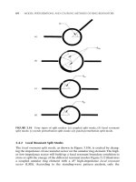
er. Figure 6.1 depicts the relative position of the MAC protocol within a simplified proto-
col stack.
The specific functions associated with a MAC protocol vary according to the system
requirements and application. For example, wireless broadband networks carry data
streams with stringent quality of service (QoS) requirements. This requires a complex
MAC protocol that can adaptively manage the bandwidth resources in order to meet these
demands. Design and complexity are also affected by the network architecture, communi-
cation model, and duplexing mechanism employed. These three elements are examined in
the rest of the section.
6.2.1 Network Architecture
The architecture determines how the structure of the network is realized and where the
network intelligence resides. A centralized network architecture features a specialized
node, i.e., the base station, that coordinates and controls all transmissions within its cover-
age area, or cell. Cell boundaries are defined by the ability of nodes to receive transmis-
sions from the base station. To increase network coverage, several base stations are inter-

connected by land lines that eventually tie into an existing network, such as the public
switched telephone network (PTSN) or a local area network (LAN). Thus, each base sta-
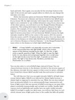
tion also plays the role of an intermediary between the wired and wireless domains. Figure
6.2 illustrates a simple two-cell centralized network.
120
WIRELESS MEDIA ACCESS CONTROL
User Application User Application
IP
Datalink
MAC Protocol
Network Interface
TCP UDP
Logical Link Control
Routing
Figure 6.1 Position of the MAC protocol within a simplified protocol stack.
Communication from a base station to a node takes place on a downlink channel, and
the opposite occurs on an uplink channel. Only the base station has access to a downlink
channel, whereas the nodes share the uplink channels. In most cases, at least one of these
uplink channels is specifically assigned to collect control information from the nodes. The
base station grants access to the uplink channels in response to service requests received
on the control channel. Thus, the nodes simply follow the instructions of the base station.
The concentration of intelligence at the base station leads to a greatly simplified node
design that is both compact and energy efficient. The centralized control also simplifies
QoS support and bandwidth management since the base station can collect the require-
ments and prioritize channel access accordingly. Moreover, multicast packet transmission
is greatly simplified since each node maintains a single link to the base station. On the
other hand, the deployment of a centralized wireless network is a difficult and slow
process. The installation of new base stations requires precise placement and system con-
figuration along with the added cost of installing new landlines to tie them into the exist-
ing system. The centralized system also presents a single point of failure, i.e., no base sta-

tion equals no service.
The primary characteristic of an ad hoc network architecture is the absence of any pre-
defined structure. Service coverage and network connectivity are defined solely by node
proximity and the prevailing RF propagation characteristics. Ad hoc nodes communicate
directly with one another in a peer-to-peer fashion. To facilitate communication between
distant nodes, each ad hoc node also acts as a router, storing and forwarding packets on
behalf of other nodes. The result is a generalized wireless network that can be rapidly de-
ployed and dynamically reconfigured to provide on-demand networking solutions. An ad
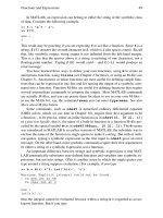
hoc architecture is also more robust in that the failure of one node is less likely to disrupt
network services. Figure 6.3 illustrates a simple ad hoc network.
Although a generic architecture certainly has its advantages, it also introduces several
new challenges. All network control, including channel access, must be distributed. Each
ad hoc node must be aware of what is happening in its environment and cooperate with
other nodes in order to realize critical network services. Considering that most ad hoc sys-
tems are fully mobile, i.e., each node moves independently, the level of protocol sophisti-
cation and node complexity is high. Moreover, each ad hoc node must maintain a signifi-
6.2 GENERAL CONCEPTS 121
Wireless Link
Base Station
Cell
Wired Link
Node
Figure 6.2 Centralized network architecture.
cant amount of state information to record crucial information such as the current network
topology.
Given its distributed nature, channel access in an ad hoc network is achieved through
the close cooperation between competing nodes. Some form of distributed negotiation is
needed in order to efficiently allocate channel resources among the active nodes. The
amount of overhead, both in terms of time and bandwidth resources, associated with this
negotiation will be a critical factor of the overall system performance.

6.2.2 Communication Model
The communication model refers to the overall level of synchronization present in the
wireless system and also determines when channel access can occur. There are different
degrees of synchronization possible; however, there are only two basic communication
models. The synchronous communication model features a slotted channel consisting of
discrete time intervals (slots) that have the same duration. With few exceptions, these slots
are then grouped into a larger time frame that is cyclically repeated. All nodes are then
synchronized according to this time frame and communication occurs within the slot
boundaries.
The uniformity and regularity of the synchronous model simplifies the provision of
quality of service (QoS) requirements. Packet jitter, delay, and bandwidth allotment can all
be controlled through careful time slot management. This characteristic establishes the syn-
chronous communication model as an ideal choice for wireless systems that support voice
and multimedia applications. However, the complexity of the synchronization process de-
pends on the type of architecture used. In a centralized system, a base station can broadcast
a beacon signal to indicate the beginning of a time frame. All nodes within the cell simply
listen for these beacons to synchronize themselves with the base station. The same is not
true of an ad hoc system that must rely on more sophisticated clock synchronization mech-
anisms, such as the timing signals present in the global positioning system (GPS).
The asynchronous communication model is much less restrictive, with communication
taking place in an on-demand fashion. There are no time slots and thus no need for any
global synchronization. Although this certainly reduces node complexity and simplifies
communication, it also complicates QoS provisioning and bandwidth management. Thus,
an asynchronous model is typically chosen for applications that have limited QoS require-
122
WIRELESS MEDIA ACCESS CONTROL
Node
Wir
e
l

ess
Link
Figure 6.3 Ad hoc network architecture.
ments, such as file transfers and sensor networks. The reduced interdependence between
nodes also makes it applicable to ad hoc network architectures.
6.2.3 Duplexing
Duplexing refers to how transmission and reception events are multiplexed together. Time
division duplexing (TDD) alternates transmission and reception at different time instants
on the same frequency band, whereas frequency division duplexing (FDD) separates the
two into different frequency bands. TDD is simpler and requires less sophisticated hard-
ware, but alternating between transmit and receive modes introduces additional delay
overhead. With enough frequency separation, FDD allows a node to transmit and receive
at the same time, which dramatically increases the rate at which feedback can be obtained.
However, FDD systems require more complex hardware and frequency management.
6.3 WIRELESS ISSUES
The combination of network architecture, communication model, and duplexing mecha-
nism define the general framework within which a MAC protocol is realized. Decisions
made here will define how the entire system operates and the level of interaction between
individual nodes. They will also limit what services can be offered and delineate MAC
protocol design. However, the unique characteristics of wireless communication must also
be taken into consideration. In this section, we explore these physical constraints and dis-
cuss their impact on protocol design and performance.
Radio waves propagate through an unguided medium that has no absolute or observ-
able boundaries and is vulnerable to external interference. Thus, wireless links typically
experience high bit error rates and exhibit asymmetric channel qualities. Techniques such
as channel coding, bit interleaving, frequency/space diversity, and equalization increase
the survivability of information transmitted across a wireless link. An excellent discussion
on these topics can be found in Chapter 9 of [1]. However, the presence of asymmetry
means that cooperation between nodes may be severely limited.
The signal strength of a radio transmission rapidly attenuates as it progresses away

from the transmitter. This means that the ability to detect and receive transmissions is de-
pendent on the distance between the transmitter and receiver. Only nodes that lie within a
specific radius (the transmission range) of a transmitting node can detect the signal (carri-
er) on the channel. This location-dependent carrier sensing can give rise to so-called hid-
den and exposed nodes that can detrimentally affect channel efficiency. A hidden node is
one that is within range of a receiver but not the transmitter, whereas the contrary holds
true for an exposed node. Hidden nodes increase the probability of collision at a receiver,
whereas exposed nodes may be denied channel access unnecessarily, thereby underutiliz-
ing the bandwidth resources.
Performance is also affected by the signal propagation delay, i.e., the amount of time
needed for the transmission to reach the receiver. Protocols that rely on carrier sensing are
especially sensitive to the propagation delay. With a significant propagation delay, a node
may initially detect no active transmissions when, in fact, the signal has simply failed to
6.3 WIRELESS ISSUES 123
reach it in time. Under these conditions, collisions are much more likely to occur and sys-
tem performance suffers. In addition, wireless systems that use a synchronous communica-
tions model must increase the size of each time slot to accommodate propagation delay.
This added overhead reduces the amount of bandwidth available for information transmis-
sion.
Even when a reliable wireless link is established, there are a number of additional hard-
ware constraints that must also be considered. The design of most radio transceivers only al-
low half-duplex communication on a single frequency. When a wireless node is actively
transmitting, a large fraction of the signal energy will leak into the receive path. The power
level of the transmitted signal is much higher than any received signal on the same frequen-
cy, and the transmitting node will simply receive its own transmission. Thus, traditional col-
lision detection protocols, such as Ethernet, cannot be used in a wireless environment.
This half-duplex communication model elevates the role of duplexing in a wireless
system. However, protocols that utilize TDD must also consider the time needed to
switch between transmission and reception modes, i.e., the hardware switching time.
This switching can add significant overhead, especially for high-speed systems that op-

erate at peak capacity [2]. Protocols that use handshaking are particularly vulnerable to
this phenomenon. For example, consider the case when a source node sends a packet and
then receives feedback from a destination node. In this instance, a turnaround time of 10
␮s and transmission rate of 10 Mbps will result in an overhead of 100 bits of lost chan-
nel capacity. The effect is more significant for protocols that use multiple rounds of mes-
sage exchanges to ensure successful packet reception, and is further amplified when
traffic loads are high.
6.4 FUNDAMENTAL MAC PROTOCOLS
Despite the great diversity of wireless systems, there are a number of well-known MAC
protocols whose use is universal. Some are adapted from the wired domain and others are
unique to the wireless one. Most of the current MAC protocols use some subset of the fol-
lowing techniques.
6.4.1 Frequency Division Multiple Access (FDMA)
FDMA divides the entire channel bandwidth into M equal subchannels that are sufficient-
ly separated (via guard bands) to prevent cochannel interference (see Figure 6.4). Ignoring
the small amount of frequency lost to the guard bands, the capacity of each subchannel is
C/M, where C is the capacity associated with the entire channel bandwidth. Each source
node can then be assigned one (or more) of these subchannels for its own exclusive use.
To receive packets from a particular source node, a destination node must be listening on
the proper subchannel. The main advantage of FDMA is the ability to accommodate M si-
multaneous packet transmissions (one on each subchannel) without collision. However,
this comes at the price of increased packet transmission times, resulting in longer packet
delays. For example, the transmission time of a packet that is L bits long is M · L/C. This is
M times longer than if the packet was transmitted using the entire channel bandwidth. The
124
WIRELESS MEDIA ACCESS CONTROL
exclusive nature of the channel assignment can also result in underutilized bandwidth re-
sources when a source node momentarily lacks packets to transmit.
6.4.2 Time Division Multiple Access (TDMA)
TDMA divides the entire channel bandwidth into M equal time slots that are then orga-

nized into a synchronous frame (see Figure 6.5). Conceptually, each slot represents one
channel that has a capacity equal to C/M, where C is again the capacity of the entire chan-
nel bandwidth. Each node can then be assigned one (or more) time slots for its own exclu-
sive use. Consequently, packet transmission in a TDMA system occurs in a serial fashion,
6.4 FUNDAMENTAL MAC PROTOCOLS 125
Time
Frequency
1
2
M
Figure 6.4 Frequency division multiple access.
Figure 6.5 Time division multiple access.
21
M
Time
Frequency
with each node taking turns accessing the channel. Since each node has access to the en-
tire channel bandwidth in each time slot, the time needed to transmit a L bit packet is then
L/C. When we consider the case where each node is assigned only one slot per frame,
however, there is a delay of (M – 1) slots between successive packets from the same node.
Once again, channel resources may be underutilized when a node has no packet(s) to
transmit in its slot(s). On the other hand, time slots are more easily managed, allowing the
possibility of dynamically adjusting the number of assigned slots and minimizing the
amount of wasted resources.
6.4.3 Code Division Multiple Access (CDMA)
While FDMA and TDMA isolate transmissions into distinct frequencies or time instants,
CDMA allow transmissions to occupy the channel at the same time without interference.
Collisions are avoided through the use of special coding techniques that allow the infor-
mation to be retrieved from the combined signal. As long as two nodes have sufficiently
different (orthogonal) codes, their transmissions will not interfere with one another.

CDMA works by effectively spreading the information bits across an artificially broad-
ened channel. This increases the frequency diversity of each transmission, making it less
susceptible to fading and reducing the level of interference that might affect other systems
operating in the same spectrum. It also simplifies system design and deployment since all
nodes share a common frequency band. However, CDMA systems require more sophisti-
cated and costly hardware, and are typically more difficult to manage.
There are two types of spread spectrum modulation used in CDMA systems. Direct se-
quence spread spectrum (DSSS) modulation modifies the original message by multiplying
it with another faster rate signal, known as a pseudonoise (PN) sequence. This naturally in-
creases the bit rate of the original signal and the amount of bandwidth that it occupies. The
amount of increase is called the spreading factor. Upon reception of a DSSS modulated sig-
nal, a node multiplies the received signal by the PN sequence of the proper node. This in-
creases the amplitude of the signal by the spreading factor relative to any interfering signals,
which are diminished and treated as background noise. Thus, the spreading factor is used to
raise the desired signal from the interference. This is known as the processing gain.
Nevertheless, the processing gain may not be sufficient if the original information signal
received is much weaker than the interfering signals. Thus, strict power control mechanisms
are needed for systems with large coverage areas, such as a cellular telephony networks.
Frequency hopping spread spectrum (FHSS) modulation periodically shifts the trans-
mission frequency according to a specified hopping sequence. The amount of time spent
at each frequency is referred to as the dwell time. Thus, FHSS modulation occurs in two
phases. In the first phase, the original message modulates the carrier and generates a nar-
rowband signal. Then the frequency of the carrier is modified according to the hopping se-
quence and dwell time.
6.4.4 ALOHA Protocols
In contrast to the elegant solutions introduced so far, the ALOHA protocols attempt to
share the channel bandwidth in a more brute force manner. The original ALOHA protocol
126
WIRELESS MEDIA ACCESS CONTROL
was developed as part of the ALOHANET project at the University of Hawaii [3].

Strangely enough, the main feature of ALOHA is the lack of channel access control.
When a node has a packet to transmit, it is allowed to do so immediately. Collisions are
common in such a system, and some form of feedback mechanism, such as automatic re-
peat request (ARQ), is needed to ensure packet delivery. When a node discovers that its
packet was not delivered successfully, it simply schedules the packet for retransmission.
Naturally, the channel utilization of ALOHA is quite poor due to packet vulnerability.
The results presented in [4] demonstrate that the use of a synchronous communication
model can dramatically improve protocol performance. This slotted ALOHA forces each
node to wait until the beginning of a slot before transmitting its packet. This reduces the
period during which a packet is vulnerable to collision, and effectively doubles the chan-
nel utilization of ALOHA. A variation of slotted ALOHA, known as p-persistent slotted
ALOHA, uses a persistence parameter p, 0 < p < 1, to determine the probability that a
node transmits a packet in a slot. Decreasing the persistence parameter reduces the num-
ber of collisions, but increases delay at the same time.
6.4.5 Carrier Sense Multiple Access (CSMA) Protocols
There are a number of MAC protocols that utilize carrier sensing to avoid collisions with
ongoing transmissions. These protocols first listen to determine whether there is activity
on the channel. An idle channel prompts a packet transmission and a busy channel sup-
presses it. The most common CSMA protocols are presented and formally analyzed in [5].
While the channel is busy, persistent CSMA continuously listens to determine when
the activity ceases. When the channel returns to an idle state, the protocol immediately
transmits a packet. Collisions will occur when multiple nodes are waiting for an idle chan-
nel. Nonpersistent CSMA reduces the likelihood of such collisions by introducing ran-
domization. Each time a busy channel is detected, a source node simply waits a random
amount of time before testing the channel again. This process is repeated with an expo-
nentially increasing random interval until the channel is found idle.
The p-persistent CSMA protocol represents a compromise between persistent and non-
persistent CSMA. In this case, the channel is considered to be slotted but time is not syn-
chronized. The length of each slot is equal to the maximum propagation delay, and carrier
sensing occurs at the beginning of each slot. If the channel is idle, the node transmits a

packet with probability p, 0 < p < 1. This procedure continues until either the packet is
sent, or the channel becomes busy. A busy channel forces a source node to wait a random
amount of time before starting the procedure again.
6.5 CENTRALIZED MAC PROTOCOLS
In this section, we provide an overview of two of the most prevalent centralized wireless
networks. Cellular telephony is the most predominant form of wireless system in current
operation. Wireless ATM is generating a lot of interest for its ability to deliver broadband
multimedia services across a wireless link. Each system will be briefly highlighted and the
MAC protocol will be examined.
6.5 CENTRALIZED MAC PROTOCOLS 127
6.5.1 Cellular Telephony
The advanced mobile phone system (AMPS) is an FDMA-based cellular system [6]. The
system features 832 full-duplex channels that are grouped into control and data channels.
Each cell has a full-duplex control channel dedicated to system management, paging,
and call setup. There are also 45–50 data channels that can be used for voice, fax, or data.
The base station grants access to a data channel in response to a call setup request sent on
the control channel. A data channel remains assigned to a specific node until it is relin-
quished or the node moves outside the current cell. Access to the control channel is deter-
mined using a CSMA-based MAC protocol. The base station periodically broadcasts the
status of the control channel, and a node transmits its setup request (possibly in contention
with other nodes) when the control channel is idle. Collisions among setup requests are re-
solved using randomized retransmissions.
The IS-136 cellular system is a digital version of the AMPS system [7]. As such, it oper-
ates within the same spectrum using the same frequency spacing of the original AMPS sys-
tem. Each data channel is then slotted and a time frame of six slots is used. This allows the
system to support multiple users within a single AMPS data channel. An assignment of one
slot per frame can support a total of six users transmitting at a rate of 8.1 kb/s. Higher data
rates can be achieved by successively doubling the number of assigned slots up to a maxi-
mum of 48.6 kb/s. Channel access remains relatively unchanged from the original AMPS
system.

The IS-95 cellular system is a CDMA-based wireless network in which all the base sta-
tions share a common frequency band with individual transmissions being distinguished
by their PN sequences [8]. Strict power control ensures that all transmitted signals reach
the base station with the same power level. This allows a more equitable sharing of the
system power resources while minimizing systemwide cochannel interference. However,
the equalized power levels make it difficult to determine when a node is about to leave one
cell and enter another. A node must communicate with multiple base stations simultane-
ously, allowing it to measure the relative signal quality of each base station. Handover is
then made to the base station with the best signal characteristics. This type of system re-
quires complex and costly hardware both within the base stations and nodes.
Cdma2000 is the third generation (3G) version of the IS-95 cellular system. Cdma2000
is backward compatible with the current system, allowing legacy users to be accommodat-
ed in future 3G systems. Many other proposed 3G cellular systems have also adopted a
CDMA interface. This includes the 3G version of GSM known as the universal mobile
telecommunications services (UMTS) [9].
6.5.2 Wireless ATM
Asynchronous transfer mode (ATM) is a high-performance connection-oriented switching
and multiplexing technology that uses fixed-sized packets to transport a wide range of in-
tegrated services over a single network. These include voice, video, and multimedia ser-
vices that have different QoS requirements. The ability to provide specific QoS services is
one of the hallmarks of ATM. Wireless ATM is designed to extend these integrated ser-
vices to the mobile user.
128
WIRELESS MEDIA ACCESS CONTROL