Báo cáo y học: "PopMod: a longitudinal population model with two interacting disease states" ppsx
Bạn đang xem bản rút gọn của tài liệu. Xem và tải ngay bản đầy đủ của tài liệu tại đây (359.95 KB, 15 trang )
BioMed Central
Page 1 of 15
(page number not for citation purposes)
Cost Effectiveness and Resource
Allocation
Open Access
Methodology
PopMod: a longitudinal population model with two interacting
disease states
Jeremy A Lauer*
1
, Klaus Röhrich
2
, Harald Wirth
2
, Claude Charette
3
,
Steve Gribble
3
and Christopher JL Murray
1
Address:
1
Global Programme on Evidence for Health Policy (GPE/EQC), World Health Organization, 1211 Geneva 27, SWITZERLAND,
2
Creative
Services, Technoparc Pays de Gex, 55 rue Auguste Piccard, 01630 St Genis Pouilly, FRANCE and
3
Statistics Canada, R.H Coats Building, Holland
Avenue, Ottawa, Ontario K1A 0T6, CANADA
Email: Jeremy A Lauer* - ; Klaus Röhrich - ; Harald Wirth - ;
Claude Charette - ; Steve Gribble - ; Christopher JL Murray -
* Corresponding author
Abstract
This article provides a description of the population model PopMod, which is designed to simulate
the health and mortality experience of an arbitrary population subjected to two interacting disease
conditions as well as all other "background" causes of death and disability. Among population
models with a longitudinal dimension, PopMod is unique in modelling two interacting disease
conditions; among the life-table family of population models, PopMod is unique in not assuming
statistical independence of the diseases of interest, as well as in modelling age and time
independently. Like other multi-state models, however, PopMod takes account of "competing risk"
among diseases and causes of death.
PopMod represents a new level of complexity among both generic population models and the
family of multi-state life tables. While one of its intended uses is to describe the time evolution of
population health for standard demographic purposes (e.g. estimates of healthy life expectancy),
another prominent aim is to provide a standard measure of effectiveness for intervention and cost-
effectiveness analysis. PopMod, and a set of related standard approaches to disease modelling and
cost-effectiveness analysis, will facilitate disease modelling and cost-effectiveness analysis in diverse
settings and help make results more comparable.
Introduction
Historical background and analytical context
Measuring population health has been inseparable from
the modelling of population health for at least three hun-
dred years. The first accurate empirically based life table –
a population model, albeit a simple one – was constructed
by Edmund Halley in 1693 for the population of Breslau,
Germany.[1] However, the 1662 life table of John Graunt,
while less rigorously based on empirical mortality data,
represented a reasonably good approximation of life ex-
pectancy at birth in the seventeenth century.[2] Indeed,
because of Graunt's strong a priori assumptions about age-
specific mortality, his life table could be said to represent
the first population model. Recently, multi-state life ta-
bles, which explicitly model several population transi-
tions, have become a common tool for demographers,
health economists and others, and a considerable body of
theory has been developed for their use and interpreta-
tion.[3–5] Despite the substantial complexity of existing
multi-state models, a recent publication has highlighted
Published: 26 February 2003
Cost Effectiveness and Resource Allocation 2003, 1:6
Received: 25 February 2003
Accepted: 26 February 2003
This article is available from: />© 2003 Lauer et al; licensee BioMed Central Ltd. This is an Open Access article: verbatim copying and redistribution of this article are permitted in all
media for any purpose, provided this notice is preserved along with the article's original URL.
Cost Effectiveness and Resource Allocation 2003, 1 />Page 2 of 15
(page number not for citation purposes)
the advantages of so-called "dynamic life tables", in which
age and time would be modelled independently.[6]
Mathematical and computational constraints are no long-
er serious obstacles to solving complex modelling prob-
lems, although the empirical data required for complex
models are. In particular, multi-state models present data
requirements that can rapidly exceed empirical knowl-
edge about real-world parameter values, and in many cas-
es, the input parameters for such models are therefore
subject to uncertainty. Nevertheless, even with substantial
uncertainty, such models can provide robust answers to
interesting questions. Indeed, the work of John Graunt
demonstrates the practical value of results obtained with
even purely hypothetical parameter values.
PopMod, one of the standard tools of the WHO-CHOICE
programme />, is the first
published example of a multi-state dynamic life table.
Like other multi-state models, PopMod takes account of
"competing risk" among diseases, causes of death and
possible interventions. However, PopMod represents a
new level of complexity among both generic population
models and the family of multi-state life tables. Among
population models with a longitudinal dimension, Pop-
Mod is unique in modelling two distinct and possibly in-
teracting disease conditions; among the life-table family
of population models, PopMod is unique in not assuming
statistical independence of the diseases of interest, as well
as in modelling age and time independently.
While one of PopMod's intended uses is to describe the
time evolution of population health for standard demo-
graphic purposes (e.g. estimates of healthy life expectan-
cy), another prominent aim is to provide a standard
measure of effectiveness for intervention and cost-effec-
tiveness analysis. PopMod, and a related set of standard
approaches to disease modelling and cost-effectiveness
analysis used in the WHO-CHOICE programme, facilitate
disease modelling and cost-effectiveness analysis in di-
verse settings and help make results more comparable.
However, the implications of a tool such as PopMod for
intervention analysis and cost-effectiveness analysis is a
relatively new area with little published scholarship. Most
published cost-effectiveness analysis has not taken a pop-
ulation approach to measuring effectiveness, and when
studies have done so they have generally adopted a
steady-state population metric.[7] Relatively little pub-
lished research has noted the biases of conventional ap-
proaches when used for resource allocation.[8]
Despite similarities in some of the mathematical tech-
niques,[9] this paper does not consider transmissible dis-
ease modelling.
Basic description of the model
PopMod simulates the evolution in time of an arbitrary
population subject to births, deaths and two distinct dis-
ease conditions. The model population is segregated into
male and female subpopulations, in turn segmented into
age groups of one-year span. The model population is
truncated at 101 years of age. The population in the first
group is increased by births, and all groups are depleted
by deaths. Each age group is further subdivided into four
distinct states representing disease status. The four states
comprise the two groups with the individual disease con-
ditions, a group with the combined condition and a group
with neither of the conditions. The states are denominat-
ed for convenience X, C, XC and S, respectively. The state
entirely determines health status and disease and mortal-
ity risk for its members. For example, X could be ischae-
mic heart disease, C cerebrovascular disease, XC the joint
condition and S the absence of X or C.
State members undergo transitions from one group to an-
other, they are born, they get sick and recover, and they
die. The four groups are collectively referred to as the total
population T, births are represented as the special state B,
and deaths as the special state D. A diagram for the first
age group is shown in Figure 1 (notation used is explained
in the section Describing states, populations and transitions
between states). In the diagram, states are represented as
boxes and flows are depicted as arrows. Basic output con-
sists of the size of the population age-sex groups reported
at yearly intervals. From this output further information is
derived. Estimates of the severity of the states X, C, XC and
S are required for full reporting of results, which include
standard life-table measures as well as a variety of other
summary measures of population health.
There now follows a more technical description of the
model and its components, broken down into the follow-
ing sections: describing states, populations and transi-
tions between states; disease interactions; modelling
mechanics; and output interpretation. The article con-
cludes with a discussion of the relation of PopMod to oth-
er modelling strategies, plus a consideration of the
implications, advantages and limitations of the approach.
Describing states, populations and transitions
between states
Describing states and populations
In the full population model depicted in Figure 1, six age-
and-sex specific states (X, C, XC, S, B and D) are distin-
guished. However, births B and deaths D are special states
in the sense that they only feed into or absorb from other
states (while the states X, C, XC and S both feed into and
absorb from other states). Special states are not treated
systematically in the following, which focuses on the
Cost Effectiveness and Resource Allocation 2003, 1 />Page 3 of 15
(page number not for citation purposes)
"reduced form" of the model consisting of the states X, C,
XC, and S.
States are not distinguished from their members; thus, "X"
is used to mean alternatively "disease X" or "the popula-
tion group with disease X", according to context. The sec-
ond meaning is equivalent to the prevalence count for the
population group.
For the differential equation system, states/groups are al-
ways denoted in the strict sense: "X" means "state X only"
or "the population group with only X". However, in deriv-
ing input parameters (described more fully below in the
section Disease interactions) from observed populations, it
is convenient to describe groups in a way that allows for
the possibility of "overlap". For example in Figure 2, the
area "X" might be understood to mean either "the popu-
lation group with X including those members with C as
well" (i.e. the entire circle X) or the "the population group
with only X" (i.e. the circle minus the region overlapping
with circle C).
Since these two valid meanings imply different uses of no-
tation, the following conventions are adopted:
• The differential equations expressions X, C, XC and S re-
fer only to disjoint states (or groups).
• The logical operator "~ "means "not", thus "~ X" is the
state "not X" (or "the group without X").
• The logical expressions denoted in the left-hand column
of Table 1 have the meaning and alternative description
indicated in the two right-hand columns.
Figure 1
The differential equations model.
B
X
C
S
XC
D
r
x
→
xc
m
r
s
→
c
r
c
→
s
r
xc
→
x
r
c
→
xc
r
x
→
s
r
xc
→
c
r
s
→
x
m
+
f
c
m + f
x
m
+
f
xc
bin
0
T
Cost Effectiveness and Resource Allocation 2003, 1 />Page 4 of 15
(page number not for citation purposes)
Figure 2
A schematic for describing observed populations.
Table 1: Alternative ways to describe populations.
Logical expression Meaning Differential equations expression
~ X~ C Population group with neither X nor C S
X~ C Population group with X but not C, i.e. with X only X
~ XC Population group with C but not X, i.e. with C only C
~ X Population group without X S + C
~ C Population group without C S + X
X Total population group with X X + XC
C Total population group with C C + XC
S Susceptible population S
XC Population with both X and C XC
T Total population T
Cost Effectiveness and Resource Allocation 2003, 1 />Page 5 of 15
(page number not for citation purposes)
Prevalence rates (p) describe populations (i.e. prevalence
counts) as a proportion of the total, for example:
p
X
= X/T, p
C
= C/T, p
XC
= XC/T, p
S
= S/T. (1)
Here, prevalence is presented in terms of the disjoint pop-
ulations X, C and XC, and the notation from the right-
hand column of Table 1 is used. In the section Disease
interactions, we discuss the case of overlapping
populations.
A prevalence rate is always interpretable as a probability,
but a probability is not always interpretable as a preva-
lence. The lower-case Greek letter pi (π) is used through-
out this article to denote probability. Probabilities can be
used to describe populations as noted in Table 2.
Describing transitions between states
In the differential equation system, transitions (i.e. flows)
between population groups are modelled as instantane-
ous rates, represented in Figure 1 as labelled arrows. In-
stantaneous rates are frequently called hazard rates, a
usage generally adopted here (demographers tend to refer
to instantaneous rates as "hazards" or as "forces" – e.g.
force of mortality – although epidemiologists commonly
use the term "rate" with the same meaning). A transition
hazard is labelled here h, frequently with subscript arrows
denoting the specific state transition.
In PopMod terminology, the transitions X→D, C→D and
XC→D are partitioned into two parts, one of which is the
cause-specific fatality hazard f due to the condition X, C or
XC, and the other which is the non-specific death hazard
(due to all other causes), called background mortality m:
h
X→D
= f
X
+ m (2a)
h
C→D
= f
C
+ m (2b)
h
XC→D
= f
XC
+ m (2c) (2)
h
S→D
= m. (2d)
PopMod consequently allows for up to twelve exogeneous
hazard parameters (Table 3).
Transition hazards
A time-varying transition hazard is denoted h(t). The haz-
ard expresses the proportion of the at-risk population (dP/
P) experiencing a transition event (i.e. exiting the popula-
tion) during an infinitesimal time dt:
h(t) = - (1/P)·dP/dt. (3)
"Instantaneous rate" means the transition rate obtaining
during the infinitesimal interval dt, that is, during the in-
stant in time t. If an instantaneous rate does not vary, or
its small fluctuations are immaterial to the analysis, Pop-
Mod parameters can be interpreted as average hazards
without prejudice to the model assumptions.
Average hazards can be approximated by counting events
∆P during a period ∆t and dividing by the population time
at risk. If for practical purposes the instantaneous rate
does not change within the time span, the approximate
average hazard can be used as an estimate for the underly-
ing instantaneous rate:
- (1/P)·dP/dt ≈ -∫dP / ∫Pdt ≈ - ∆P / (P·∆ t), (4)
where ∆P = ∫dP is the cumulative number of events occur-
ring during the interval ∆t, and ∫Pdt ≈ P·∆t is the
corresponding population time at risk. Time at risk is ap-
proximated by multiplying the mid-interval population
(P) by the length of the interval ∆t.
For example, if ten deaths due to disease X (∆P = 10) occur
in a population with approximately one million years of
time at risk (P·∆t = 1,000,000), an approximation of the
instantaneous rate h
X→D
(t) is given by:
h
X→D
(t) ≈ ∆P / P·∆t = 10 / 1,000,000 = 0.00001. (5)
Note that while eq. (3) and eq. (4) are equivalent in the
limit where ∆t→0, the approximation in eq. (4) will result
in large errors when rates are high. This is discussed in the
section Proportions and hazard rates, and an alternative for-
mula for deducing average hazard is proposed in eq. (9).
The quantity in eq. (4) has units "deaths per year at risk",
and is often called a "cause-specific mortality hazard". For
the same population and deaths, but restricting attention
Table 2: Probability of finding members of population groups in PopMod.
Symbol Description
π
X
Probability of finding a member of T that is a member of X with random selection.
π
C
Probability of finding a member of T that is a member of C with random selection.
π
XC
Probability of finding a member of T that is a member of XC with random selection.
Cost Effectiveness and Resource Allocation 2003, 1 />Page 6 of 15
(page number not for citation purposes)
to the group with disease X (where, for example, P·∆t =
10,000) the calculated hazard will be larger:
h
X→D
(t) ≈ ∆P / P·∆t = 10 / 10,000 = 0.001. (6)
The quantity in eq. (6) has the same units as that in eq.
(5), but is a "case fatality hazard". Note that the same tran-
sition events (e.g. "dying of disease X") can be used to de-
fine different hazard rates depending on which
population group is considered.
Proportions and hazard rates
Integration by parts of eq. (3) shows that the proportion
of the population experiencing the transition in the time
interval ∆t (i.e. the "incident proportion") is given by:
If the hazard is constant, that is, if h(t) = h(t
0
) = h, ∫dt = ∆t
and the integral collapses. The incident proportion is then
written:
The incident proportion can always be interpreted as the
average probability that an individual in the population
will experience the transition event during the interval
(e.g. for mortality, this probability can be written π
P→D
=
∆P/P). The qualification "average" is dropped if individu-
als in P are homogeneous with respect to transition risk
during the interval.
Even if the hazard is not constant, eq. (8) can be rear-
ranged to give an alternative (exact) formula for calculat-
ing the equivalent constant hazard h yielding ∆P
transitions in the interval ∆t:
However, if the true hazard is constant during the interval,
the "equivalent constant hazard" equals the "average haz-
ard" and the "instantaneous rate". The same identity ap-
plies when fluctuations in the underlying hazard are of no
practical importance. PopMod requires the assumption
that hazards are constant within the unit of its standard re-
porting interval, defined by convention as one year.
Note that series expansion of exp{-h·∆t} or ln{1-∆P/P}
shows that, for values of h·∆t << 1 and ∆P/P << 1, the
equivalent constant hazard is well approximated by the
time-normalized incident proportion, and vice versa, as in
eq. (4):
Case-fatality hazards
Case-fatality hazards f
X
, f
C
, and f
XC
are defined with re-
spect to the specific populations X, C and XC, respectively:
Table 3: Transition hazards in the population model.
Hazard Description State transition
h
S→X
incidence hazard S→X
h
X→S
remission hazard X→S
h
S→C
incidence hazard S→C
h
C→S
remission hazard C→S
h
X→D
case fatality hazard X→D
h
C→D
case fatality hazard C→D
h
XC→D
case fatality hazard XC→D
h
T→D
background mortality hazard T→D
h
C→XC
incidence hazard C→XC
h
XC→C
remission hazard XC→C
h
X→XC
incidence hazard X→XC
h
XC→X
remission hazard XC→X
∆
∆
P
Pt
ht t
t
tt
()
exp ( )d
0
17
0
0
=− −
()
+
∫
∆
∆
P
P
ht
=−
()
−⋅
18e.
h
P
P
t=− −
()
ln / .19
∆
∆
h
t
P
P
≈
()
1
10
∆
∆
.
Cost Effectiveness and Resource Allocation 2003, 1 />Page 7 of 15
(page number not for citation purposes)
Mortality hazards
Mortality hazards are defined with respect to the entire
population, where cause-specific mortality hazards are
conditional on cause of death:
The background mortality rate m is defined as the instan-
taneous rate of deaths due to causes other than X or C.
Disease interactions
PopMod is typically used to simulate the evolution of a
population subjected to two disease conditions, where
health status, health risk and mortality risk are condition-
al on disease state. Health status, health risk and mortality
risk are plausibly conditional on disease state when the
two primary disease conditions X and C interact. Such in-
teractions can be analysed from various perspectives, for
example, common risk factors, common treatments, com-
mon prognosis; however, the primary perspective adopt-
ed here for the pupose of analysis is that of "common
prognosis", by which is meant that the two conditions
mutually influence prevalence, incidence, remission and
mortality risk.
A previously cited example was that of ischaemic heart
disease (X) and cerebrovascular disease (C): it is well
known that individuals with either heart disease or stroke
history have lower health status and higher mortality risk
than individuals with neither of these conditions, and
that individuals with heart disease are at increased risk for
stroke and vice versa.
Furthermore, individuals with history of both heart dis-
ease and stroke (XC) are known to have higher mortality
risk and lower health status than either individuals with
only one of the disease histories or those with neither.
However, in this example as in many others, information
about the joint condition (heart disease and stroke) is
scarce relative to information about the two individual
conditions (heart disease or stroke). The obvious reason
for this is that the population group with the joint condi-
tion is smaller in size and has a lower life expectancy, re-
ducing opportunities for data collection.
The presimulation problem
One of PopMod's guiding principles, therefore, is that
while an analyst has access to information about basic pa-
rameter values for the conditions X and C (i.e. prevalence
rates and incidence, remission and either case-fatality or
cause-specific mortality hazards), the same is not general-
ly true for the joint condition XC. Thus, more or less by
construction, the modelling situation is one in which data
for the joint condition are scarce or unavailable, and must
consequently be derived from data known for the individ-
ual conditions.
An important implication is that the data available for the
individual conditions (X and C) will be reported in terms
of overlapping populations. Where specifically noted,
therefore, the notation in the left-hand column of Table 1
(Logical expressions) is used in the following, with the
particular implication that "X", for example, means "the
population group with X including those members with C
as well" (i.e. "X + XC" in differential equations
terminology).
Once parameter values for the joint condition are deter-
mined, the minimum set of parameters required for pop-
ulation simulation are known. The parameter-value
problem – referred to here as the presimulation problem,
since its solution must precede population simulation per
se – can be divided into two principal parts: one concern-
ing the prevalence rates defining the intial conditions
(stocks) of the differential equations system, and the oth-
er the transition hazards defining its flows. These stocks
and flows together make up the initial scenario of the
population model. A cross-sectional approach is adopted
in which deriving these two kinds of parameters values for
the initial scenario are treated as separate problems.
The analytics of these derivations largely depend on which
of a range of possible assumptions is made about the in-
teractions of the two principal conditions. The simplest
possible assumption is essentially an assumption of non-
interaction (statistical independence). Since an under-
standing of the non-interacting case is an essential starting
point for more complex interactions, it is discussed first.
f
t
X
X
f
t
C
C
f
t
X
C
XC
=− −
()
=− −
()
=−
1
111
1
112
1
∆
∆
∆
∆
∆
ln ,
ln ,
lln .113−
()
∆XC
XC
m
t
T
T
m
t
T
T
TD
tot
X
X
=− −
()
=− −
()
→
1
114
1
115
∆
∆
∆
∆
ln ,
ln ,
mm
t
T
T
TD
C
C
=− −
()
→
1
116
∆
∆
ln .
Cost Effectiveness and Resource Allocation 2003, 1 />Page 8 of 15
(page number not for citation purposes)
The independence assumption
Prevalence for the joint group
When conditions X and C are statistically independent,
the joint prevalence is the product of the individual (mar-
ginal) prevalences:
p
XC
= p
X
·p
C
. (17)
Transition hazards for the joint group
Independence implies that the hazards for the group with
X or C are equal to the corresponding hazards for the
group without X or C (in eq. (18) populations are denoted
in differential equations (disjoint) notation from the
right-hand column of Table 1):
h
XC→C
= h
X→S
h
XC→X
= h
C→S
(18)
h
C→XC
= h
S→X
h
X→XC
= h
S→C
Joint case fatality hazard
The probabilities and for an individual
in group X or C to die of cause X or C, respectively, during
an interval ∆t are:
So the joint probability for someone in the
group XC dying of either X or C is given by the laws of
probability:
Although individuals in the joint group XC are at risk of
death from either X or C, or from other causes, the proba-
bility framework requires the assumption that they do not
die of simultaneous causes (i.e. there is no cause of death
"XC").
The combined case-fatality rate f
XC
is thus:
f
XC
= f
X
+ f
C
. (21)
This simple addition rule can be generalized to situations
with more than two independent causes of death.
Background mortality hazard
The "background mortality hazard" m expresses mortality
risk for population T due to any cause of death other than
X and C. The "independence assumption" claims m is in-
dependent of these causes, in other words, that m acts
equally on all groups (in eqs. (22–25) populations are de-
noted in differential equations notation from the right-
hand column of Table 1):
m·T = m·(S + X + C + XC) = m·S + m·X + m·C + m·XC.
(22)
The total ("all cause" or "crude") death hazard for the
population is written m
tot
. The following identity express-
es the constraint that deaths in population T equal the
sum of deaths in populations S, X, C and XC:
m
tot
·T = m·S + (m + f
X
)·X + (m + f
C
)·C + (m + f
XC
)·XC.
(23)
Thus:
m
tot
·T = m·(S + X + C + XC) + f
X
·X + f
C
·C + f
XC
·XC
= m·T + f
X
·X + f
C
·C + (f
X
+ f
C
)·XC (24)
=m·T + f
X
·(X + XC) + f
C
·(C + XC).
Since by definition group X or C contributes no deaths
due to cause C or X, respectively:
f
C
·(C + XC) = m
C
·T,
f
X
·(X + XC) = m
X
·T, (25)
so:
m
tot
·T = m·T + m
X
·T + m
C
·T. (26)
and:
m = m
tot
- m
X
- m
C
. (27)
Likewise, this rule is generalizable to scenarios with more
than three (m, X, C) independent causes of death.
Relaxing the independence assumption
As noted in the introduction, one of the primary reasons
for the introduction of PopMod was to model disease in-
teractions in a longitudinal population model. Modelling
interactions requires relaxing the assumption of
independence.
π
X
X
D→
π
C
C
→ D
ππ
X
X
D
X
X
C
C
C
C
and
→→
=− = =− =
−⋅
→
−⋅
(e ) (e )11
ft
XD
ft
C
X
X
C
C
D
∆
∆
∆∆
→
()
D
.19
π
XC
X or C
→ D
πππππ
XC X D C X D C
X or C X C X C
X
→ →→→→
−⋅
=+−⋅
()
=−
DDD
f
(e1
∆∆
∆
∆
∆
∆
∆
t
ft
ft
ft
ft
ft
)(e)(e)(e)
ee
+− −− ⋅−
=−
=
−⋅
−⋅
−⋅
−⋅
−⋅
111
1
C
X
C
X
C
11
1
20
−
≡−
()
−+⋅
−⋅
e
e
()ff t
ft
XC
XC
∆
∆
Cost Effectiveness and Resource Allocation 2003, 1 />Page 9 of 15
(page number not for citation purposes)
In the presimulation of the "stocks and flows" required for
the initial scenario, three areas of interaction for the
health states X and C can be distinguished. Having X (C)
may make it more or less likely to:
(1) have C (X),
(2) acquire or recover from C (X),
(3) die from C (X).
Note that while interaction (1) could alternatively be con-
sidered the cumulative result of interactions (2) and (3) in
the past, this is not the approach adopted here.
Interaction (1): Prevalence of the joint group
In this and subsequent sections except where noted, we re-
vert to the notation from the left-hand column of Table 1.
Table 4 shows six possible cases for calculating prevalence
of the joint group depending on the type of information
known about the disease interaction. The probability no-
tation π is used for prevalence, where π
X|C
is the probabil-
ity of having disease X among those who have disease C
and π
X
and π
C
are short forms for π
X|T
and π
C|T
. Relative
risk (RR) is defined here as a ratio of probabilities (risk ra-
tio), for example, RR
C|X
= π
C|X
/ π
C|~X
is the probability of
having X if C is present over the probability of having X if
C is not present.
Calculations for case 1 follow directly from the assump-
tion of independence. Cases 2 and 3 follow directly from
the definition of conditional probability. Cases 4 and 5
are derived as follows. Since the probability of belonging
to the joint group is independent of which disease group
is conditioned on, it is clear that:
π
XC
= π
X|C
·π
C
= π
C|X
·π
X
. (28)
Using the definition of conditional probability, we write:
π
X
= π
X|C
·π
C
+ π
X|~C
·π
~C
, and
π
C
= π
C|X
·π
X
+ π
C|~X
·π
~X
. (29)
Now supposing RR
X|C
or RR
C|X
is known, solving either
for π
X|C
or π
C|X
and substituting the result into eq. (29)
and solving again for π
X|C
and π
C|X
yields:
π
X|C
= π
X
/ (π
C
+ π
~C
/ RR
X|C
), and
π
C|X
= π
C
/ (π
X
+ π
~X
/ RR
C|X
). (30)
So again using the definition of conditional probability:
π
XC
= π
X
·π
C
/ (π
C
+ π
~C
/ RR
X|C
), and
π
XC
= π
C
·π
X
/ (π
X
+ π
~X
/ RR
C|X
). (31)
Recalling 1 - π
X
= π
~X
and 1 - π
C
= π
~C
, the required expres-
sions in Table 4 are obtained.
The factor k in case 6 is an arbitrary multiplier that increas-
es or reduces the prevalence of group XC compared to
what would be obtained under independence, and lies be-
tween 0 and 1 if having one disease reduces the probabil-
ity of having the other, and between 1 and MAX(1/π
C
, 1/
π
X
) if having one disease makes it more likely to have the
other. Upper bounds on k are easy to derive using the fact
that π
XC
= π
X
= π
C
when X and C are obligate symbiotes.
The six cases span a range of information availability
about interaction of X and C on the prevalence of the joint
condition:
• Case 1 assumes independence (no interaction).
• Case 2 and 3 assume conditional prevalence is known.
• Case 4 and 5 assume relative risk is known.
• Case 6 assumes a potentiation (or protection) factor can
be defined.
Interaction (2): Incidence and remission for the joint group
For incidence hazard, we write i and for remission hazard,
r. Consistent with "overlapping populations", unless spe-
cifically noted, hazards are understood as "total hazards",
Table 4: Options for calculating overlap probability π
XC
.
Case
π
XC
calculated as
Comment
1 π
C
·π
X
C and X are independent
2 π
C|X
·π
X
C and X interact and π
C|X
or π
X|C
is known.
3 π
X|C
·π
C
4 π
C
·π
X
/ [π
C
+ (1 - π
C
) / RR
X|C
] C and X are dependent and the relative risk RR
X|C
or RR
C|X
is known.
5 π
X
·π
C
/ [π
X
+ (1 - π
X
) / RR
C|X
] X (C) either potentiates, or protects from, C (X).
6 π
X
·π
C
·k
Cost Effectiveness and Resource Allocation 2003, 1 />Page 10 of 15
(page number not for citation purposes)
that is, i
X
includes all incidence to X regardless of whether
C is also present in the population at risk. Conditional
hazards are denoted i
X|~C
or i
X|C
to signify "incidence to X
in the group without C" and "incidence to X in the group
with C", respectively.
Consider total incidence i
X
for the initial scenario. The
product of total incidence to X and the total population
without X (~X) must be equal to the sum of the products
of the conditional incidences (i
X|~C
, i
X|C
) and the condi-
tional populations (~X~C, ~XC):
i
X
·(~X) = i
X|~C
·(~X~C) + i
X|C
·(~XC). (32)
Dividing by total population T yields:
and replacing population ratios by the corresponding
prevalence rates yields:
i
X
·π
~X
= i
X|~C
·π
~X~C
+ i
X|C
·π
~XC
. (34)
Dividing both sides by π
~X
yields the following expression
for i
X
:
where:
π
~X
= π
~X~C
+ π
~XC
. (36)
It is therefore clear that total incidence to X is a weighted
average of the conditional incidences, where the weights
are the proportions of the population without X parti-
tioned according to C status.
Recall that, in terms of the differential equations notation
from the right-hand column of Table 1, π
~X
= π
C
+ π
S
,
π
~X~C
= π
S
and π
~XC
= π
C
, the values of which are deter-
mined according to one of the six cases defined above in
interaction (1). Thus, when total hazard i
X
is known, eq.
(34) has only two unknowns (i
X|~C
and i
X|C
). Clearly, if
information on one or both conditional hazards is avail-
able, interaction (2) with respect to i
X
is fully character-
ized for the initial scenario.
However, the guiding principle of the presimulation
problem was that information on the non-overlapping
populations (e.g. direct observation of the conditional
hazards) is relatively scarce. When this is true, the un-
known conditional hazards must remain undetermined
unless one of the following three rate ratios (RR) is known
or can be approximated:
A similar situation applies to the total hazards i
C
, r
C
, and
r
X
for the initial scenario, that is, eq. (34) is one of a family
of equations representing the relation between the total
disease hazards and the corresponding conditional haz-
ards for subpopulations:
i
X
·π
~X
= i
X|~C
·π
~X~C
+ i
X|C
·π
~XC
i
C
·π
~C
= i
C|~X
·π
~X~C
+ i
C|X
·π
X~C
(38)
r
X
·π
X
= r
X|~C
·π
X~C
+ r
X|C
·π
XC
r
C
·π
C
= r
C|~X
·π
~XC
+ r
C|X
·π
XC
.
Note that, with respect to the initial scenario, eq. (38)
forms a simultaneous system with eq. (31) – or one of the
other methods of calculating π
XC
noted in Table 4 – and
the system has a unique numerical solution whenever
enough parameter values are known, that is, assuming the
four total hazards are known, if one of the three following
rate ratios (or its inverse) is known for each hazard:
Interaction (3): Mortality for the joint group
This interaction concerns causes of death. We assume that
the all-cause mortality hazard m
tot
and the total (i.e. over-
lapping) case-fatality hazards f
X
and f
C
are known. It fol-
lows that:
f
X
·π
X
= f
X|~C
·π
X~C
+ f
X|C
·π
XC
, and
f
C
·π
C
= f
C|~X
·π
~XC
+ f
C|X
·π
XC
. (40)
i
X
T
i
XC
T
i
XC
T
X X|~C X|C
⋅=⋅ +⋅
()
(~ )
()
(~ ~ )
()
(~ )
()
,33
ii i
XX|~C
XC
X
X|C
XC
X
=⋅ +⋅
()
π
π
π
π
~~
~
~
~
,35
RR i
i
i
RR i
i
i
RR i
i
i
() , () , ()
~
~
X
XC
XC
X
XC
X
X
XC
X
or . 37
12 3
== =
()
RR i
i
i
RR i
i
i
RR i
i
i
RR i
() , () , () ,
(
~
~
X
XC
XC
X
XC
X
X
XC
X
C
or and
12 3
== =
)),() ,(),
()
~
12 3
1
== =
=
i
i
RR i
i
i
RR i
i
i
RR r
r
CX
C~X
C
CX
C
C
CX
C
X
or and
XXC
XC
X
XC
X
X
XC
X
C
CX
C
or and
r
RR r
r
r
RR r
r
r
RR r
r
r
~
~
,() , () ,
()
23
1
==
=
~~
~
,() , () .
X
C
CX
C
C
CX
C
or RR r
r
r
RR r
r
r
23
39
==
()
Cost Effectiveness and Resource Allocation 2003, 1 />Page 11 of 15
(page number not for citation purposes)
Following a derivation similar to that in eqs (19) – (21),
one can show that, given total case-fatality hazards f
X
and
f
C
, the case-fatality hazard for the joint condition is the
sum of the conditional hazards:
f
XC
= f
X|C
+ f
C|X
(41)
Further, since:
m
X
·T = f
X|~C
·(X ~ C) + f
X|C
·(XC), and
m
C
·T = f
C|~X
·(~XC) + f
C|X
·(XC), (42)
so:
m
X
= f
X|~C
·π
X~C
+ f
X|C
·π
XC
, (43)
and:
m
C
= f
C|~X
·π
~XC
+ f
C|X
·π
XC
. (44)
In other words, the cause-specific mortality hazards are
weighted averages of the conditional case-fatality hazards,
where weights are the proportions of the total population
according to disease status regarding the other condition.
It remains true that:
m = m
tot
- m
X
- m
C
, (45)
as in eq. (27).
Other interactions
Another interaction might involve relaxing the assump-
tion of independence between background mortality haz-
ard m and case-fatality hazards f
X
and f
C
. However, in
cases where such dependence is suspected or known, it
may be possible to "work around" it by choosing appro-
priate definitions for X and C. For example, to take the is-
chaemic heart disease (X) and stroke (C) example,
suppose it is important for the research question to ac-
count for the fact that individuals with X or C are also at
increased risk of mortality from other selected causes of
death such as cardiac failure. While one approach might
be to introduce a new box for cardiac failure, within the
current structure of PopMod, the onus is effectively on the
analyst to take into account such increased risk of back-
ground mortality by modifying the way state C is defined
and by adjusting the corresponding incidence and case-fa-
tality rates. For example, state C could be defined as
"stroke and all other conditions (including cardiac fail-
ure) at increased risk due to heart disease". Another type
of exception to the general rule of independence between
background mortality and cause-specific mortality would
be the existence of any common causal modifiers of m, f
X
and f
C
, for example, the allocation of health-care
expenditure.
Modelling mechanics
Initial conditions
PopMod describes population evolution conditional on
initial conditions that define the state of the system at
some initial time. These initial conditions consist of the
population distribution in non-overlapping terms. If po-
tentially overlapping populations (i.e. descriptions from
the left hand side of Table 1) are considered, when the to-
tal prevalences p
X
and p
C
are known the non-overlapping
population distribution can be fully determined by deter-
mining the prevalence of the joint group. Methods for this
are discussed in the section Disease interactions.
Runge-Kutta method
The differential equation system is determined by its ini-
tial conditions and its parameters. An algebraic descrip-
tion of PopMod differential equation system – using
notation from the right-hand side of Table 1 – is:
dS/dt = -(h
S→X
+ h
S→C
+ h
S→D
)·S + (h
X→S
)·X + (h
C→S
)·C
(46a)
dX/dt = -(h
X→S
+ h
X→XC
+ h
X→D
)·X + (h
S→X
)·S + (h
X-
C→X
)·XC (46b)
dC/dt = -(h
C→X
+ h
C→XC
+ h
C→D
)·C + (h
S→C
)·S + (h
X-
C→C
)·XC (46c) (46)
dXC/dt = -(h
XC→X
+ h
XC→C
+ h
XC→D
)·XC + (h
X→XC
)·X +
(h
C→XC
)·C (46d)
dD/dt = (h
S→D
)·S + (h
X→D
)·X + (h
C→D
)·C + (h
X-
C→D
)·XC (46e)
Under specified conditions, which apply here, such a dif-
ferential equation system has a unique solution, and the
solution can be expressed in terms of the eigenvalues and
eigenvectors of the 5 × 5 coefficient matrix.[10]
Since finding the required eigenvalues and eigenvectors is
here equivalent to solving a fifth-degree polynomial equa-
tion, specialized solution algorithms – and access to a
substantial amount of processor time – will generally be
required. An attractive alternative is therefore the use of
numerical techniques, since they yield solutions more
cheaply, and without requiring custom routines.
In PopMod, the evolution of the population in time is ap-
proximated by a 4
th
-order Runge-Kutta method, or, op-
tionally, by a 5
th
-order Runge-Kutta method.[10] The
relevant time step is defined as a fraction of the standard
reporting interval (the number of divisions of the basic re-
Cost Effectiveness and Resource Allocation 2003, 1 />Page 12 of 15
(page number not for citation purposes)
porting interval must in principle be divisible by 3, but to
allow for the possibility of starting with mid-year values in
the first year, the number of divisions must be divisible by
6 and the minimum number of divisions is fixed at 12).
Note that an n
th
-order numerical method will in general
provide useful results so long as the differentials are small-
er than n
th
-order in the chosen time step.
Each population age- and sex group is modelled as a sep-
arate system, and age is updated by taking end-of-year so-
lution values for the "age = α " system as the initial values
for the "age = α + 1" system in the subsequent model year.
A 4
th
-order Runge-Kutta method provides solutions to
differential equations of the type:
dy
i
(x)/dx = f
i
(x, y
i
(x)), (47)
and is defined by the ansatz (Euler method) that:
y
i
(x + ∆x) = y
i
(x) + ∆x·f
i
(x, y
i
(x)), (48)
where:
y
i
(x + ∆x) = y
i
(x) + (k
1i
+ 2k
2i
+ 2k
3i
+ k
4i
)/6 + O(∆x
5
), and
k
1i
= ∆x·f
i
(x, y
i
)
k
2i
= ∆x·f
i
(x + ∆x/2, y
i
+ k
1i
/2) (49)
k
3i
= ∆x·f
i
(x + ∆x/2, y
i
+ k
2i
/2)
k
4i
= ∆x·f
i
(x + dx, y
i
+ k
3i
).
Note that here x = t, y
i
= S, X, C, XC and D and that the dif-
ferential equations (46a-46e) are not explicitly time de-
pendent, that is, f
i
(t, y
i
(t)) = f
i
(y
i
(t)).[10]
Output interpretation
Standard PopMod output reports P(t) for each population
group as end-of-interval (e.g. year-end) values, corre-
sponding to the standard life table quantity l
x
. An impor-
tant derived quantity also included in output is the time
at risk experienced by the group during the interval (∫P(t)
dt), corresponding to the life table quantity L
x
(sometimes
called "life-years" or "person-years").
For a constant population, population time at risk is cal-
culated P·∆t. For PopMod populations, population time
at risk for the interval b - a is calculated:
When the quantity resulting from eq. (50) with units "per-
son-years" is divided by the length of the time interval
with units "years", average population size for the interval
( , with units "persons") is obtained:
thus conforms to the definition of the expected value
of the function P(t) on the interval b - a. Since b - a is by
convention one year (or "chronon" etc.), the normaliza-
tion to the interval b - a means dividing by 1. Thus, since
in this case the numerical quantity is unchanged, substi-
tuting different reporting units yields two equally valid in-
terpretations for the same output:
(1) the average population size = E [P(t)] during the in-
terval ∆t, or
(2) the population time at risk P
LY
experienced during the
interval ∆t.
Interpretation (1) also corresponds to average (count)
prevalence for the population.
When transition rates are "small" (i.e. the differentials are
approximately linear), average population can be inter-
preted as mid-interval population. Under the same as-
sumptions, mid-year population provides a good estimate
of population time at risk.
PopMod numerically evaluates P
LY
with a standard New-
ton-Cotes formula for 4-point closed quadrature, some-
times also called Simpson's 3/8-rule.[11] The quadrature
formula relies on the values of P(t) determined by the
Runge-Kutta method at multiples of the chosen time step.
Since these values involve numerical estimation error,
there is no simple expression for the order of accuracy of
the different output values reported in PopMod.[10]
Discussion
Advantages of the approach
PopMod combines features of existing models (see be-
low) with the possibility to analyse several disease states.
It explicitly analyses time evolution and, even more
importantly, abandons the constraint of independence of
disease states.
A primary advantage of the approach adopted in PopMod
is the separate modelling of age and time, and the type of
bias inherent in models that do not do so has been previ-
ously pointed out.[7] Moreover, it has been independent-
P Ptt X Xtt
LY
a
b
LY
a
b
=
()
=
() ( )
∫∫
d, d.for example 50
ˆ
P
ˆ
()d .P
ba
Pt t
a
b
=
−
()
∫
1
51
ˆ
P
ˆ
P
Cost Effectiveness and Resource Allocation 2003, 1 />Page 13 of 15
(page number not for citation purposes)
ly noted that, without this feature, life-table measures are
constrained to adopt – somewhat artificially – either a
"period" or a "cohort" perspective.[6] The other chief ad-
vantage of PopMod is the ability to deal with heterogene-
ity of disease and mortality risk by modelling up to four
disease states. No previous published generic population
model has combined both these features. Note, however,
that if disease conditions are independent, and popula-
tion-dependent effects are not of interest, a multi-state
life-table approach should probably be adopted.[20]
A further advantage of PopMod is the introduction of a
systematic analytical approach to the modelling of disease
interactions. This by itself represents a relatively impor-
tant advance, as modellers have until now been con-
strained to model only independent conditions.
Furthermore, in spite of the increased informational de-
mands made by a four-state system, the modelled func-
tional dependency between X-related hazards conditional
on C status, and vice versa, reduces the number of exoge-
nous hazards that need to be directly observed. This is of
substantial practical importance, since, while direct obser-
vation of conditional hazards usually requires a cohort
study, it will often be possible to obtain estimates of the
required rate ratios from more common case-control stud-
ies [21].
Related models
In addition to the multi-state life table family,[3,4] two
additional families of mathematical models have some
similarity to PopMod. One family comprises the class of
models sometimes called incidence, prevalence and mor-
tality (IPM) models.[12–14] Another family (with until
now one member) is that of published population mod-
els, in particular Prevent.[15–18]
IPM models per se have no population or age structure;
they can be conceived of as stationary population models
(i.e. models of a population in equilibrium, where the
numbers of births and deaths in an age group are equal).
However, DisMod, probably the IPM model in most com-
mon use, [12] has gone through several versions, and the
current version allows for hazard trend analysis that relies
on modelling a full population structure based on one-
year age groups. Notwithstanding, IPM models analyse
only a single disease condition in isolation, and, while
Prevent was explicitly designed to analyse a full popula-
tion cohort structure, it also analyses only a single disease
condition.
Multi-state life tables analyse multiple disease states but
published versions have invariably required the assump-
tion of independence across diseases. In addition, multi-
state life tables implicitly impose a stationary population
assumption by not independently modelling population
time and age.
Averaging and its implications
In all compartmental models, of which differential equa-
tions models are one type, it is assumed that health and
mortality risk are conditional on disease state. In light of
the seemingly infinite diversity of real phenomena, this
assumption invariably results in "compression", that is,
the imposition of artificial homogeneity. In many cases,
compression can be considered a necessary simplifying as-
sumption for the modelling exercise, but in other cases,
heterogeneity must be explicitly modelled to avoid the
phenomenon of confounding. In a differential equations
system, modelling heterogeneity of disease and mortality
risk amounts to introducing additional disease states.
Thus, PopMod, with four disease states, respresents a sub-
stantial increase in complexity over population models
modelling only two disease states (e.g. diseased and
healthy). PopMod of course includes the two-disease-state
model as a special case.
There is also heterogeneity other than of disease and mor-
tality risk. In particular, although real populations change
in integer steps at discrete moments in time, a differential
equation system represents this process in continuous
time. However, this approximation is in general accepta-
bly good when a large number of individuals comprise
the population of interest. Moreover, an implication of
representing age in a discrete number of statistical bins is
modelling a birth-year cohort as though it had a single av-
erage age. If births are distributed uniformly throughout
the year, the average birthday of the cohort is the mid-year
point, and there is no serious objection to this procedure.
However, if the cohort average birthday is not be the mid-
year point, PopMod's modelled age will differ from the
true average age.
It is assumed that conditional hazards are constant within
a single reporting interval (e.g. one year), which will in
principle be problematic for conditions with high initial
case-fatality, for example heart attack (or stroke). This sort
of problem can be addressed by defining condition C as
''acutely fatal cases'' and condition X as ''long-term
survivors''. Similarly, for conditions of determinate dura-
tion (e.g. pregnancy), use of a constant hazard rate for ''re-
mission'' will result in an exponential distribution of
waiting time for transition out of the state, whereas a uni-
form distribution of waiting time is what would be
wanted.
All compartmental population models are fundamentally
simplifications of reality by means of a system of reduced
dimensionality. The mathematical concept of "projec-
tion" is useful: the simplified system can be thought of as
Cost Effectiveness and Resource Allocation 2003, 1 />Page 14 of 15
(page number not for citation purposes)
a "least-squares approximation" to the higher-order real
system.[19] The validity of input parameter values and the
accuracy of the solution method determine the actual
goodness of fit realized in a particular model. Neverthe-
less, compression applies to every modelled variable in a
differential equations model. Other modelling approach-
es, such as microsimulation, require much less compres-
sion, so the user who wishes to avoid compression
systematically should consider adopting the microsimula-
tion approach.
Types of error in PopMod
Sources of error in PopMod can be divided into three
types:
(1) Model (or "projection") error due to analysing a sim-
plified system instead of the full one. Model error includes
the characterization of scenarios for disease interaction.
(2) Numerical error due to obtaining approximate solu-
tion values with numerical techniques.
(3) Parameter error due to uncertainty about observed or
derived parameter values.
The 5
th
-order Runge-Kutta method provides an estimate
of the local truncation error inherent in the 4
th
-order nu-
merical technique. Monte-Carlo analysis of distributions
around transition rates can be used to examine parameter
uncertainty. However, comparison with a more complex
model would be necessary for quantification of model er-
ror. A way of investigating the impact of model error
would be to construct progressively more realistic and
complex models. A spectrum of models, from least to
most complex, can thus be imagined, where the "most
complex" and necessarily imaginary model has a one-to-
one relation to real system it represents. The difference be-
tween the results of two adjacent models in such a series
would be an expression of model error analogous to the
estimate of numerical truncation error afforded by the
next-higher-order numerical method.
Although intuitively natural and mathematically valid, in
most situations it would be impractical to quantify model
error in this laborious way. Nevertheless, model error
may, in certain data-rich cases, be estimated by ''predict-
ing'' outcomes for which numerical data are available for
comparison but which are not used as inputs.
Limiting assumptions
Although any state transitions are in principle possible,
PopMod assumes that transitions S→XC and X→C do not
occur. This is because such transitions can be thought of
as the simultaneous occurrence of two transitions (for ex-
ample, S→XC equals S→X plus X→XC). Note that this
does not imply events S→XC and X→C cannot occur
within a single reporting interval; rather, it just means the
mathematics of PopMod do not represent simultaneous
events. A similar feature is the absence of a modelled
cause of death "XC".
However, the non-modelled transition S→XC can be im-
agined if someone in state S simultaneously acquires X
and C as a result of, say, very high levels of common risk
factors (i.e. someone who suffers a simultaneous heart at-
tack and stroke because of high blood pressure and cho-
lesterol). If such a "simultaneous event" results in
mortality, one could potentially speak of a cause of death
"XC". Similarly, the non-modelled transition X→C could
occur if there were "perfect interference" between two
diseases such that acquiring C caused immediate remis-
sion from X. If either of these cases is important, PopMod
can miss important dynamics.
Authors' contributions
JL devised the methodology, implemented the conceptual
and technical development of PopMod, including coordi-
nation of co-authors' contributions, and drafted and re-
vised the manuscript. KR and HW contributed to the
development of the methodology, drafted certain sections
and revised the manuscript. CC and SG contributed to the
development of the methodology, revised mathematical
formulae throughout, and revised the manuscript. CM
provided the initial idea for the model and also contribut-
ed technical modifications throughout development of
the main ideas presented in this paper. All authors ap-
proved the final manuscript.
Conflict of interest
None declared.
Acknowledgements
Reviewers Nico Nagelkerke of Leiden University and Louis Niessen of Er-
asmus University Rotterdam are gratefully acknowledged. Jan Barendregt
and Sake de Vlas of Erasmus University Rotterdam also offered valuable
comments and suggestions for revision. David Evans, Raymond Hutubessy,
Stephen Lim, Colin Mathers, Sumi Mehta, Josh Salomon and Tessa Tan
Torres of the World Health Organization, Geneva, are also gratefully ac-
knowledged for their comments and contributions.
References
1. Shryock HS and Siegel JS The life table. In: The methods and materials
of demography (Edited by: Stockwell EG) Orlando, FL, Academic Press
1976, 250
2. Hacking I The emergence of probability. Cambridge, Cambridge
University Press 1975,
3. Barendregt JJ and Bonneux L Degenerative disease in an aging
population: models and conjectures. Enschede, Netherlands,
Febodruke 1998,
4. Manton KG and Stallard E Chronic disease modelling. London,
Charles Griffin 1988,
5. Schoen R Modelling multigroup populations. New York and Lon-
don, Plenum Press 1987,
6. Barendregt JJ Incidence- and prevalence-based summary
measures of population health (SMPH): making the twain
Publish with Bio Med Central and every
scientist can read your work free of charge
"BioMed Central will be the most significant development for
disseminating the results of biomedical research in our lifetime."
Sir Paul Nurse, Cancer Research UK
Your research papers will be:
available free of charge to the entire biomedical community
peer reviewed and published immediately upon acceptance
cited in PubMed and archived on PubMed Central
yours — you keep the copyright
Submit your manuscript here:
/>BioMedcentral
Cost Effectiveness and Resource Allocation 2003, 1 />Page 15 of 15
(page number not for citation purposes)
meet. In: Summary measures of population health: concepts, ethics, meas-
urement and applications (Edited by: Murray CJL, Lopez AD, Salomon JA,
Mathers CD) Geneva, World Health Organization 2002, 221-231
7. Preston SH Health indices as a guide to health sector planning:
a demographic critique. In: The epidemiological transition, policy and
planning implications for developing countries (Edited by: Gribble JN, Pres-
ton SH) Washington DC, National Academy Press 1993,
8. Murray CJL Rethinking DALYs. In: The Global Burden of Disease: A
comprehensive assessment of mortality and disability from diseases, injuries,
and risk factors in 1990 and projected to 2020 (Edited by: Murray CJ,
Lopez AD) Cambridge, MA, Harvard University Press 1996, 1-98
9. Anderson RM and May RM Infectious diseases of humans: dy-
namics and control. Oxford, Oxford University Press 1991,
10. Lambert JD Numerical methods for ordinary differential sys-
tems: the initial value problem. Chichester, Wiley 1991,
11. Ralston A and Rabinowitz P A first course in numerical analysis.
Mineola, NY, Dover 1965,
12. Kruijshaar ME, Barendregt JJ and Hoeymans N The use of models
in the estimation of disease epidemiology. Bull World Health
Organ 2002, 80:622-628
13. Murray CJ and Lopez AD Quantifying disability: data, methods
and results. Bull World Health Organ 1994, 72:481-494
14. Barendregt JJ, Baan CA and Bonneux L An indirect estimate of the
incidence of non-insulin-dependent diabetes mellitus. Epide-
miology 2000, 11:274-279
15. Mooy JM and Gunning-Schepers LJ Computer-assisted health im-
pact assessment for intersectoral health policy. Health Policy
2001, 57:169-177
16. Bronnum-Hansen H How good is the Prevent model for esti-
mating the health benefits of prevention? J Epidemiol Community
Health 1999, 53:300-305
17. Gunning-Schepers LJ Models: instruments for evidence based
policy. J Epidemiol Community Health 1999, 53:263
18. Bronnum-Hansen H and Sjol A [Prediction of ischemic heart dis-
ease mortality in Denmark 1982–1991 using the simulation
model Prevent]. Ugeskr Laeger 1996, 158:4898-4904
19. Strang G Linear algebra and its applications. San Diego, CA, Har-
court Brace Jovanovich 1988,
20. Barendregt JJ, van Oortmarssen GJ, van Hout BA, Van Den Bosch JM
and Bonneux L Coping with multiple morbidity in a life table.
Math Popul Stud 1998, 7:29-49
21. Rothman KJ and Greenland S Modern epidemiology. Philadelphia,
PA, Lippincott Williams and Wilkins 1998,