Báo cáo y học: " Research ChIP-PaM: an algorithm to identify protein-DNA interaction using ChIP-Seq data" ppsx
Bạn đang xem bản rút gọn của tài liệu. Xem và tải ngay bản đầy đủ của tài liệu tại đây (1.6 MB, 17 trang )
© 2010 Wu et al; licensee BioMed Central Ltd. This is an Open Access article distributed under the terms of the Creative Commons Attri-
bution License ( which permits unrestricted use, distribution, and reproduction in any me-
dium, provided the original work is properly cited.
Wu et al. Theoretical Biology and Medical Modelling 2010, 7:18
/>Open Access
RESEARCH
Research
ChIP-PaM: an algorithm to identify protein-DNA
interaction using ChIP-Seq data
Song Wu*
1
, Jianmin Wang
2
, Wei Zhao
1
, Stanley Pounds
1
and Cheng Cheng
1
Abstract
Background: ChIP-Seq is a powerful tool for identifying the interaction between genomic
regulators and their bound DNAs, especially for locating transcription factor binding sites.
However, high cost and high rate of false discovery of transcription factor binding sites
identified from ChIP-Seq data significantly limit its application.
Results: Here we report a new algorithm, ChIP-PaM, for identifying transcription factor
target regions in ChIP-Seq datasets. This algorithm makes full use of a protein-DNA binding
pattern by capitalizing on three lines of evidence: 1) the tag count modelling at the peak
position, 2) pa
ttern matching of a specific tag count distribution, and 3) motif searching
along the genome. A novel data-based two-step eFDR procedure is proposed to integrate
the three lines of evidence to determine significantly enriched regions. Our algorithm
requires no technical controls and efficiently discriminates falsely enriched regions from
regions enriched by true transcription factor (TF) binding on the basis of ChIP-Seq data
only. An analysis of real genomic data is presented to demonstrate our method.
Conclusions: In a comparison with other existing methods, we found that our algorithm
provides more accurate binding site discovery while maintaining comparable statistical
power.
Background
Understanding of transcriptional regulation mechanisms is of fundamental importance to
the study of biological processes such as development, drug response and disease pathogen-
esis [1]. Through modulation of gene expression patterns, the differentiation and function
of cells are tightly controlled. The on/off switch of specific gene expression is one of the
main modulating mechanisms and is mainly through the association and disassociation of
transcription factors (TFs) with their target gene promoters. Therefore, revealing the mech-
anism by which transcription factors regulate their target genes is essential to understand-
ing many important biological processes. Several methods have been developed to identify
the TF-target gene interactions and to investigate how and why cells respond to different
signals. One such method, chromatin immunoprecipitation (ChIP) on a chip (ChIP-chip), is
based on a tiling-array platform in which genomic DNA oligomers from gene promoters are
pre-fixed. The DNA fragments immuno-precipitated from cell lysate by a TF antibody
hybridize with the ChIP-chip array and TF-binding regions are identified by their high-
intensity signals. Like all other array-based methods, however, this method can detect only
targets included on the array.
* Correspondence:
1
Department of Biostatistics, St.
Jude Children's Research
Hospital, 262 Danny Thomas
Place, Memphis, TN 38105, USA
Full list of author information is
available at the end of the article
Wu et al. Theoretical Biology and Medical Modelling 2010, 7:18
/>Page 2 of 17
More recently, with the advance of next-generation sequencing (NGS) technologies,
ChIP-Seq has come into a wide use for transcription factor binding sites analysis. By
directly sequencing the DNA fragments immunoprecipitated in a ChIP experiments,
ChIP-Seq offers whole-genome coverage and greater sensitivity than the traditional
ChIP-chip assay [2]. Several analytic algorithms have been proposed for ChIP-Seq data,
including ERANGE [3], FindPeaks [4], MACS[5], SISSRs[6], CisGenome [7], QuEST [8],
Useq [9], SPP [10], PeakSeq[11], BayesPeak [12], and GLITR [13]. Most of these algo-
rithms aim to identify genomic regions enriched with ChIP-DNA fragments by using
some negative control samples to remove/normalize some of the background noise from
experimental procedures. For example, Robertson et al [2] identified the enriched
regions by detecting peaks on a tag density map, generated by extending each mapped
tag in the 3' direction to the average length of the DNA fragments in the sequenced DNA
library. The signal map is the integer count of the number of overlapping DNA frag-
ments at each nucleotide position. The control sample was generated by another ChIP-
Seq experiment using the same antibodies against the un-stimulated cells, in which the
transcription factor of interest is inactive and located in cytoplasm. Rozowsky et al [11]
used the same idea of signal map, but used the raw input DNA as the control sample.
Chen et al [14], studied a group of 13 transcription factors in E14 mouse ES cells by using
a control sample obtained from another ChIP-Seq experiment with an irrelevant anti-
body, anti-GFP.
Although these negative controls are useful, they cannot account for an important
source of noise signal - nonspecific DNA binding by TFs. This noise signal is difficult to
control, as TFs must nonspecifically bind to DNA in order to efficiently access their
unique binding sites among billions of nucleotides. Studies directly probing transcrip-
tion factor dynamics at the single-molecule level in a living cell showed that TFs spend as
much as 90% of their time non-specifically bound to and diffusing along DNAs [15]. Like
the ability to bind to specific targets, non-specific binding to DNA is a bona fide TF abil-
ity and therefore, this type of noise signal cannot be eliminated by using a negative con-
trol. A few algorithms, such as SISSRs, MACS and FindPeaks, can identify transcription
factor binding targets solely on the basis of ChIP-Seq data, without the use of control
samples. However, with the exception of SISSRs, these algorithms identify binding sites
merely by the number of tag counts within a genomic region, ignoring the forward- and
reverse- strand information. SISSRs utilizes a logic rule in which the sequenced forward
and reverse strands should lie separately on the two sides of the binding site; therefore,
the difference between the forward and reverse tag counts would change sign on the
binding site. The SISSRs algorithm usually generates significantly more binding sites
than other algorithms [6], but these may include many false discoveries, as will be shown
in later section.
Here we describe a new algorithm that incorporates the forward- and reverse-strand
information but employs it differently. Our algorithm, ChIP-PaM, is based on peak
counts modeling and pattern matching of a specific tag count distribution of forward
and reverse strands generated by protein-DNA binding, followed by de novo motif find-
ing and searching within the potential binding regions. We show that our algorithm can
greatly reduce false positive findings while maintaining or improving accuracy and sta-
tistical power for binding site discovery.
Wu et al. Theoretical Biology and Medical Modelling 2010, 7:18
/>Page 3 of 17
Results
ChIP-PaM: Scoring the Enriched Genomic Regions in ChIP-Seq Data
TF binding sites (TFBSs) usually contains a short consensus binding site (CBS) sequence,
~ 10-20 base pairs, that provides target specificity. Suppose that there is one TFBS in a
small genomic neighbourhood (e.g., < 500 bp). In a ChIP-Seq experiment, ideally all for-
ward-strand tags related to this TFBS should lie on the 5' side of the TFBS, and all
reverse-strand tags should lie on the 3' side (Figure 1A), because only fragments contain-
ing the TFBS are pulled down for sequencing. Hence, given that the maximum fragment
size selected for sequencing is d, a quantity known from ChIP-Seq experimental proce-
dures, it is expected that the region beginning d bp upstream of the TFBS and ending at
the TFBS will contain the greatest number of forward-strand tags, and the region begin-
ning at the TFBS and ending d bp downstream of the TFBS will contain the greatest
number of reverse-strand tags. If a potential TF binding region is scanned base pair by
base pair with a sliding window of width d and the unique forward and reverse tags
within the window are counted separately, the tag densities formed from forward and
reverse strands will show a pattern of peak shift along the scanned genomic region, with
the peak of one strand corresponding to the background signal of the other strand (Fig-
ure 1A, C). The tag counts at the peak position and the pattern of peak shift can be used
as physiological evidence for a TF binding. Therefore, several sequences that show good
evidence of containing the potential CBS can be aligned for de novo motif finding [16-
19].
Figure 1 Tag count distributions from the simulated and real genomic data. A. Simulated forward- and
reverse-strand count distribution for a region containing one TF binding site; B. Difference between forward-
and reverse-strand tag counts shown in panel A. C. Forward- and reverse-strand tag count distribution in an
example genomic region (from the real data application); D. Difference between forward- and reverse-strand
tag counts shown in panel C.
Wu et al. Theoretical Biology and Medical Modelling 2010, 7:18
/>Page 4 of 17
Based on the above, we propose a new algorithm, ChIP-PaM, for ChIP-Seq data analy-
sis. The method combines the tag counts at the peak position, the pattern recognition of
the forward and reverse tag shift, and de novo CBS finding. It consists of six steps that are
summarized in Figure 2 and described in detail below:
1. Identify potential binding regions (PBRs) by using a pre-specified empirical False
Discovery Rate (eFDR): The whole genome is divided into non-overlapping regions d
bp in size and the unique tags in each region are counted. The frequencies of the tag
counts are then tabulated and fitted to a Gamma-Poisson (G-P) mixture model that
can accommodate the over-dispersion of the data. The G-P model showed better fit-
ting to the real data than the frequently used Poisson model and has been used in
other software (e.g., Cis-Genome [7]). The eFDRs for different tag count thresholds,
defined as the ratio of the theoretical number of regions exceeding the thresholds by
chance from the G-P model to the number of observed regions exceeding the same
thresholds [6], can be calculated as the following
Figure 2 Sequence the ChIP-PaM algorithm.
Wu et al. Theoretical Biology and Medical Modelling 2010, 7:18
/>Page 5 of 17
where k is a count threshold, Pr(count > k) is the probability of a tag count exceeding
k in the G-P background model, N
total
is the total number of regions in the whole
genome and N
observed
(count > k) is the number of observed regions with count
exceeding k. A tag count cut-off corresponding to the pre-specified FDR rate (α, e.g.
0.5) is then determined, and the genomic regions with tag counts greater than the
cutoff are selected, and merged if adjacent, to form PBRs. The majority of the back-
ground tag signals are eliminated in this step, which can save immense amount of
computing time in the following steps.
2. Evaluate the peak tag counts for each PBR: A sliding window of width d is used to
scan the PBRs base pair by base pair and the forward and reverse tags within each
window are counted to yield the forward and reverse tag distributions similar to Fig-
ure 1A and 1C. On the basis of the fitted G-P model, a p-value is calculated for the
tag counts at the peak position within each PBR.
3. Identify the peak shift pattern from forward- to reverse- strand tag distributions: If
a PBR contains a true TFBS, the difference between the forward- and reverse- strand
tag counts will show a sinusoidal shape (Figure 1B, D). This shape is used for the pat-
tern match and is identified by pattern recognition that employs a wavelet-based
smoothing technique (see Methods for details). Dissimilarity scores comparing each
PBR to a simulated reference pattern (S
R
) are computed and ranked.
4. De novo motif finding: PBRs with high peak counts and good sinusoidal pattern of
forward to reverse tag count shift are considered as high-quality PBRs, i.e., those
most likely contain a TF binding site. The peak positions of the forward- and reverse-
strand count distribution within the high-quality PBRs are obtained, and the
genomic sequence a few bp (e.g., 20 bp) upstream and downstream of the peak sites
are retrieved to search for the de novo motif to which the TF might bind. Existing
efficient algorithms such as MEME [18] are used for motif finding. A motif search
algorithm typically generates several motifs, but only those contained by at least 25%
of the input sequences are candidate motifs. Notice that each input sequence is only
about 40 bp long; therefore it is reasonable to assume that each sequence contains
either one motif or no motif.
5. Scan potential PBRs by using the de novo motif identified: A scoring matrix formed
on the aligned consensus sequences identified in step4 is used to screen and score all
PBRs identified in step 1. The smallest p-values corresponding to the best match to
the scoring matrix in each PBR are retained as the PBR motif p-values.
6. Determine the significant regions: The PBR peak tag count p-values, pattern dis-
similarity scores, and motif p values are integrated to re-rank the PBRs. Because the
minimal p-value for the peak tag count may be as low as 10
-30
, whereas the minimal
motif p values may be only 10
-5
, the scale difference for different score distributions
is normalized. The p-values are log-transformed, rescaled to the same level and aver-
aged to re-rank the PBRs. Finally, the top (1- α) re-ordered PBRs are selected as the
significant TF target regions.
eFDR
count k N
total
N
observed
count k
=
>
>
Pr( )*
()
Wu et al. Theoretical Biology and Medical Modelling 2010, 7:18
/>Page 6 of 17
Characteristics of the ChIP-Seq data
To illustrate our method, we used a public ChIP-seq dataset (GSE12782) deposited at the
GEO by Rozowsky et al [11]. This dataset was originally analyzed by using PeakSeq. Sev-
eral characteristics of the dataset are worth noting: 1) The raw input DNA is used as con-
trol; 2) The experiments were done in female Hela S3 cells; 3) The mitochondrial
chromosomes (Chr M) were retained for sequencing; and 4) the transcription factor
studied was STAT1, a TF with many well-known downstream target genes. These char-
acteristics, while are not necessarily useful for the data analysis, provide a good opportu-
nity to assess our proposed method, including an estimate of its false negative and false
positive findings, as described below.
In the ChIP-Seq sample, ~26.7 million unique reads were mapped to the reference
genome (hg18/NCBIv36, UCSC genome browser), and in the input sample ~23.4 million
unique reads were mapped. The summary statistics are shown in Table 1. The genome-
wide coverage for the ChIP sample is 0.015 read/nt. This low sequencing coverage is typ-
ical of ChIP-Seq data because the high-affinity of TF-DNA binding averts the need for
deep sequencing on the whole genome. However, the sequenced fragments in ChIP sam-
ple and the input fragments in the control sample have very little overlap (0.75% of all
sequenced tags, Table 1). This factor could be problematic if the input sample is used as
local control, because the majority of fragments sequenced are present only in the ChIP
sample or the input sample and therefore, the input fragments cannot serve as a repre-
sentative control for ChIP data.
The mitochondrial chromosomes have been deeply sequenced due to their high copy
numbers. Most cells contain many mitochondria, and each mitochondrion contains sev-
eral copies of Chr M. Thus, Chr M copies are much more abundant than nuclear chro-
mosomes [20]. This phenomenon is observed in the example dataset; the coverage on
Chr M is ~3000 times more than that on the nuclear chromosomes from the input sam-
ple. Because mitochondrial DNA are physically separated from the nuclear STAT1 pro-
teins, they can be used as a reference to estimate the background noise from the
experimental procedure, such as the residual input DNA left in the ChIP sample. The
expected number of noise reads is estimated to be 5 million for genomic DNAs (Table 2).
However, the ChIP experiment generated about 24 million total noise reads, suggesting
that most of the background fragments in the ChIP sample come from other sources,
such as the nonspecific binding of a TF to the genome. As discussed in the Introduction,
this type of noise signals cannot be adequately resolved by using controls. This is one
challenge that promoted us to develop an algorithm independent of control samples.
In contrast to Chr M, chromosome Y (Chr Y) is another extreme with very low cover-
age, because the male Y chromosome is absent in the female Hela S3 cells. Therefore, any
enriched regions identified on the Chr Y should be considered as false positives. The fact
that some reads were mapped to Chr Y in the dataset suggests there were mapping/
sequencing errors. The reads mapped to Chr Y cannot be explained by sequence homol-
ogy to chromosome X, because only unique reads were mapped to the reference genome.
For these reasons, Chr Y serves as a perfect internal negative control. As shown in Table
1, 12.7 thousand of the 24.3 million ChIP reads were mapped to Chr Y. Given that the
length of Chr Y is 54.7 M and the whole genome is about 3 billion bps, at least 0.9 M
(3.64%) reads in the ChIP sample are predicted to be wrongly mapped or sequenced.
Wu et al. Theoretical Biology and Medical Modelling 2010, 7:18
/>Page 7 of 17
Table 1: Summary statistics of the ChIP-Seq dataset.
unique reads Copy percentage
Chr ChIP only Input only in both ChIP only Input only in both Total length ChIP Read/nt
1-22, X 24.3 M 20.9 M 0.34 M 53.3% 45.9% 0.75% 3B 0.015
Y 11 K 11.6 K 1.7 K 45.5% 47.6% 6.9% 54.7 M 0.0004
M 33 3144 16.5 K 0.17% 15.9% 83.9% 16.5 K 1.191
Shown are selected basic characteristics used in the application, comparing chromosomes 1-22 plus X (combined because they are in the 2-copy state), Chr Y, and mitochondrial chromosomes (M).
Chr Y is absent from Hela-S3 cells and indicates sequencing/mapping errors; mitochondrial chromosomes are located in cytoplasm and serve as an internal control for the nuclear chromosomes.
Wu et al. Theoretical Biology and Medical Modelling 2010, 7:18
/>Page 8 of 17
STAT1 Targets Identified by ChIP-PaM in the ChIP-Seq Dataset
We applied ChIP-PaM to the STAT1 ChIP-Seq dataset to examine the performance of
our algorithm. From the experiment procedure, the maximum fragment size was known
to be 250 bp. The whole genome was then divided into non-overlapping regions of 250
bp and the unique tags in each region were counted and tabulated into a tag count histo-
gram. This histogram resembles an empirical distribution of the background noise count
within a 250-bp region and was fitted by the G-P and Poison models (Figure 3A, B). The
comparison between the two models showed that the G-P model fits the data much bet-
ter than the Poisson model, suggesting significant dispersion of the data. Although
almost 98% of the 250-bp windows contained six or fewer unique tag reads, a close look
at the tail of the histogram and the fitted G-P density (Figure 3C) revealed significant tag
enrichment in some regions; the eFDRs for different tag count cut-offs were calculated
from these data.
With a pre-specified eFDR level of 0.5 for the count data, regions containing six or
fewer unique tag reads were eliminated, leaving 69,809 PBRs. For each PBR, a p-value
based on the count at the regional peak was calculated from the fitted G-P model, and a
dissimilarity score based on shape pattern matching was computed. These two values
were used to select 190 regions with low count p-values and the best-matched shapes,
which showed strong evidence of TF bindings. Short genomic sequences around the
peak sites (± 20 bp) in the 190 region were retrieved for de novo motif finding by using
MEME. Because each input sequence was very short (40 bp), we specified that each
sequence contained either one motif or none. A motif was identified in 112 out of 190
regions (58.9%), and all of the PBRs were then scanned for this motif by using the MAST
program [18]. The de novo motif found strongly matched the STAT1 GAS motif previ-
ously identified and validated in biological experiments [2]. From the MAST scan, a p-
value for the best motif match was obtained for each PBR. Therefore, three values were
associated with every PBR: a p-value based on count distribution (p
c
), a dissimilarity
score based on shape pattern matching (d
p
), and a p-value based on motif matching (p
m
).
The three scores were log-transformed and the log-d
p
and log-p
m
were scaled to the level
Table 2: Comparison of nuclear and cytoplasmic chromosomes.
Total Reads
Chr In ChIP In input ChIP/input ratio
Specific Reads 2356286 441471 5.3373
1-22, X Noise Reads 24285371 22585024 1.0753
E(background 4959671
noise) in ChIP* (0.2042)
M 89835 409136 0.2196
*Assuming that reads mapped to mitochondrial chromosomes (M) are due to the experimental
procedure and not to the non-specific binding of STAT1, the ChIP/input ratio for this background noise
is 21.96%. Among chromosome 1-22 and X, the expected background noise in ChIP would be
22585024*0.2196 = 4959671, which accounts for 20.42% of total noise reads.
Wu et al. Theoretical Biology and Medical Modelling 2010, 7:18
/>Page 9 of 17
of log-p
c
by regression. The PBRs were then re-ranked by averaging the three scores.
Because the original eFDR was specified to be 0.5, this suggests the true positive rate is
also 0.5 in all PBRs. Therefore, the top 34905 regions are considered significant target
regions.
The pre-specified eFDR level is somewhat arbitrary. A general rule in choosing the
eFDR is that it should be large enough to incorporate sufficient number of PBRs for re-
ranking, yet not too large to include too many noisy regions. When we used another α of
0.7 to analyze the data, 117,479 PBRs were identified and 35243 (117479*(1-0.7)) were
selected as significant regions. The number of significant regions resulting from the two
eFDRs is almost identical, as although a higher eFDR (α) yields a larger pool of PBRs, a
smaller rate of true discovery rate (1-α) offsets the initial large number in the final result.
We found that an eFDR of 0.5 is a good choice because it can generate sufficient PBRs for
further improvement while being computationally more efficient than higher eFDRs.
Comparison with Other Algorithms
We compared ChIP-PaM with SISSRs, PeakSeq and ChIP-PaM using tag counts infor-
mation only. In the STAT1 ChIP-Seq dataset described above, PeakSeq identified 36,998
significant regions [11] and SISSRs identified 85,892 significant regions. To make the
further comparison fair, we used the same number of top 36,998 regions for all algo-
rithms.
Figure 3 Model fitting of the genome-wide tag count histogram. A. Data fitted by the Gamma-Poisson
model; B. Data fitted by the Poisson model. C. The detailed right-tail fitting by the Gamma-Poisson model.
Wu et al. Theoretical Biology and Medical Modelling 2010, 7:18
/>Page 10 of 17
The false discovery rate and power are the two most important criteria in assessing a
model or algorithm. Although we do not know all of the true STAT1 binding sites in this
dataset, we do have partial knowledge to make the assessment. As mentioned before,
because Hela-S3 cells are female cells, any significant regions found on Chr Y should be
spurious. Therefore, we used the number of findings on Chr Y as a surrogate for false
discoveries. Figure 4A shows the "cumulative incidence" of findings on Chr Y as a func-
tion of the total number of significant regions. ChIP-PaM identified markedly fewer false
positives than SISSRs and PeakSeq. Compared with ChIP-PaM using the counts data
only, the incorporation of additional information about the tag distribution shape and
motif score in ChIP-PaM significantly reduced the false-positive findings.
Twenty-two genomic promoters have been experimentally validated to be regulated
and bound by STAT1 protein upon IFN-γ stimulation [2]. We used this information to
compare the power of the algorithms. As shown in Figure 4B, PeakSeq, ChIP-PaM and
ChIP-PaM using count only have almost identical "cumulative power"; they all detected a
maximum of 14 of 24 positive promoters. However, the SISSRs had the least power to
detect the known sites. In the rest 8 targets that were not identified by either method, a
detailed look at their genomic regions found that essentially no reads were mapped in
this ChIP-Seq sample, and therefore no algorithm can detect them. This suggests that
ChIP-PaM is efficient in identifying the true STAT1 targets.
We used the RefSeq to annotate the significant regions found by the three algorithms.
If an identified STAT1 binding region is located within -250 bp to 5 kp from a gene's
transcription initiation site, the gene is considered a STAT1 target. The target genes
found by the three algorithms share close similarity (Figure 5), and 2,651 of them were
identified by all three methods (Additional file 1). For the 2,651 common genes, the rank
correlation was 0.71 between ChIP-PaM and PeakSeq, 0.55 between ChIP-PaM and SIS-
SRs, and 0.52 between PeakSeq and SISSRs. These data suggest that ranking by ChIP-
PaM is more similar to ranking by SISSRs, since both used a pattern of forward and
reverse tags. However, the pattern utilized by SISSRs is somewhat too local as it cap-
tures, within a small region, the sign change of the difference between the forward and
reverse tag counts. This fact may explain why SISSRs yields a much higher false positive
rate. Two genomic examples on chromosome 1, chr1: 91,625,233 - 91,625,750 (Figure
6A) and chr1: 121,185,480 - 121,186,959 (Figure 6B), are shown to illustrate the point.
These two regions were identified as significant by SISISRs, but not by either ChIP-PaM
or PeakSeq. The overall regional pattern clearly indicates that the tag enrichments in
these two regions are not caused by TF binding; however, the rapid local sign change of
the difference between the forward and reverse tag counts causes SISSRs to consider
them as significant.
Discussion
With the advance of the next-generation techniques, ChIP-Seq experiments are expected
to be in great demand for the important biological studies of transcription regulatory
network. Therefore, more efficient models and algorithms to analyze such data are
urgently needed. Here we have proposed a new method of analysis of ChIP-Seq data that
is based on ChIP-Seq sample only and that retains and even improves the accuracy and
statistical power of binding site discovery.
Wu et al. Theoretical Biology and Medical Modelling 2010, 7:18
/>Page 11 of 17
There are four potential major mechanisms by which a region with enriched tags
might be observed in ChIP-Seq data: (1) "true positive" TF target regions; (2) focal ampli-
fication of certain genomic regions; (3) nonspecific binding of TFs to the genome; and
(4) random noise from experimental procedures. The difficulty arises in effectively sepa-
Figure 4 Comparison of ChIP-PaM with SISSRs and PeakSeq and ChIP-PaM using count data only. A.
The number of findings on Chr Y is used to compare false positive findings. B. Fourteen known STAT1 GAS tar-
get genes are used to compare the true positive findings (i.e., power).
Wu et al. Theoretical Biology and Medical Modelling 2010, 7:18
/>Page 12 of 17
rating tag enrichment resulting from (1) from those resulting from the others. Our algo-
rithm is designed to improve the accuracy of finding in each instance. The Gamma-
Poisson modeling takes account of the non-uniform noise background across the
genome and helps to model both nonspecific TF binding and random noises. The use of
pattern recognition to match a TF binding pattern will improve the detection of the true
enrichment pattern. For example, enrichment induced by focal amplification shows a
shape pattern (similar to Figure 6A) very different from that of enrichment by TF bind-
ing, and the pattern matching step of our algorithm can efficiently remove it from the
final results. Furthermore, the de novo motif finding and searching step will help elimi-
nate non-specific binding regions that do not contain the conserved motif sequences.
Because our proposed method incorporates three lines of evidence to determine the
significant TF target regions, it is more robust than other current methods and detects
fewer false positive bindings. However, it is often difficult to determine the statistical
accuracy of the findings when multiple lines of evidence are integrated. In ChIP-PaM, we
propose a novel data-based two-step FDR procedure to solve this problem. In this proce-
dure, an eFDR (α) derived from the genome-wide tag count distribution is pre-specified
to select the potential TF binding regions, and then the shape and motif information is
incorporated to re-rank the selected PBRs. As the α level controls the overall FDR and
re-ranking of the PBRs will not change it, the top (1- α) re-ordered candidate regions are
considered to be significant. This data incorporation procedure can be potentially
applied to other integrated analyses as well. Another advantage of our algorithm is that
unlike other methods, in which the average length of the ChIP fragments must be esti-
Figure 5 Venn Diagraph of genes found by the three algorithms.
Wu et al. Theoretical Biology and Medical Modelling 2010, 7:18
/>Page 13 of 17
mated, ChIP-PaM makes use of the maximum length of the fragments, which is known
from the experimental procedures. This should reduce the variation of the findings.
The entire analysis of the STAT1 example dataset took about 1.5 hours on a regular
desktop computer. Therefore, our algorithm is computationally efficient. The majority of
Figure 6 Examples of two real genomic regions that are identified as significant by SISSRs but not by
ChIP-PaM and PeakSeq. A. Chr1: 91625233- 91625750; B. Chr1: 121185480- 121186959. The red line repre-
sents forward-strand counts and the green line represents reverse-strand counts. The positive blue bars repre-
sent forward tag reads and the negative blue bars represent reverse tag reads. The broad pink line delineates
regions identified as significant by SISSRs.
Wu et al. Theoretical Biology and Medical Modelling 2010, 7:18
/>Page 14 of 17
time is spent on the shape matching and motif identification steps. Only 5 minutes is
needed to scan the PBRs and compute preliminary result from them. If the inference is
to be made on the basis of the count data and only the genome scanning part is required,
our algorithm would be extremely fast and might be algorithmically attractive for other
applications, such as epigenetic analysis of modified histone proteins [21]. Further inves-
tigation is needed in this direction.
Finally, one point worth noting is that although our algorithm requires no control sam-
ple, control samples may have an important role, depending on the scientific questions
asked. For example, if a study were to compare the binding site difference of a TF in its
"active" v.s. "inactive" form, a ChIP-Seq sample for the "inactive" TF would be a perfect
control. In this case, two ChIP-PaM analyses would be performed independently on the
two ChIP-Seq samples.
Conclusions
We propose a new algorithm, ChIP-PaM, for genome-wide identification of the tran-
scription factor target genes by using the ChIP-Seq data. Unlike other methods of ana-
lyzing ChIP-Seq data, ChIP-PaM incorporates three lines of evidences, including tag
count modeling at the peak position, pattern matching of a specific tag count distribu-
tion, and de novo motif finding and searching along the genome. A comparison with
existing methods showed that our method can greatly improve the accuracy of binding
site discovery while maintaining comparable statistical power.
Methods
Sequencing Procedures
Because information from sequencing procedures is used as parameter inputs of our
algorithm, we will briefly describe the sequencing process. In ChIP-Seq sample prepara-
tion, genomic DNAs are either sonicated or digested into random fragments and size-
selected (100-800 bp) for better sequencing accuracy. The ChIP-DNA fragments submit-
ted for sequencing are therefore within a certain range of length, e.g. 150-250 bp. Owing
to cost and technical reasons, typical tag reads acquired from sequencing apparatus for
ChIP-Seq experiments are small (~30-60 bp), and consequently reflect only the two ends
of the fragments, not the whole fragments. The end positions of fragments can be
revealed by mapping the short-read tags back to a reference genome. For single-end
sequencing, because the sequencing adaptors are ligated onto two ends of a fragment
randomly, approximately equal numbers of tags are expected to be obtained in forward
and reverse directions within a region.
Gamma-Poisson Model
If the tag reads from ChIP-Seq experiments are uniformly distributed on the genome
that is divided into equal windows of d bp, basic probabilistic considerations imply that
the distribution of unique tag counts in a certain window should obey the Poisson distri-
bution. However, since the binding affinity of a TF to the whole genome is not uniform
(i.e., specific and non-specific bindings), the ideal Poisson model will not be followed. It
is expected that the whole count data will be a mixture of Poisson distributions. Assum-
ing that the majority of DNA fragments are background signals, and that the signifi-
cantly enriched regions reside largely in the right tail of the distribution, a zero-
truncated Gamma-Poisson density can be employed as the background model for the
count data. The Gamma-Poisson model is shown as below:
Wu et al. Theoretical Biology and Medical Modelling 2010, 7:18
/>Page 15 of 17
Poisson probability mass:
Gamma density function:
Gamma-Poisson (G-P) mixture density function:
Zeros are not included in the model, as zero counts can occur simply because of non-
mappability of certain regions and therefore does not truly reflect the zero counts in the
model. The G-P model is employed to infer whether a specific region has a significantly
high count. The mean count r(1-p)/p is positively correlated with the size of the window,
i.e., the maximum fragment size d, and the sequencing depth of total number of reads
obtained, and r(1-p)/p
2
measures the dispersion of the data. There are several ways to
estimate the model parameters [22]. Here we employ the maximum likelihood method.
The maximum-likelihood estimate of the parameters (r, p) was done by using the nonlin-
ear optimization algorithms implemented in R [23].
Pattern Matching with Wavelet Smoothing
The pattern of peak shift in Figure 1A represents the difference in the tag count distribu-
tions between the forward and reverse strands. Theoretically, this difference has a sinu-
soidal shape, as illustrated in Figures 1B. The observation patterns S
PBR
are calculated for
all the PBRs that pass the initial genome scan. A reference pattern (S
R
) can also be gener-
ated from the simulation of a ChIP-Seq experiment. The S
PBR
and S
R
can then be com-
pared to calculate the dissimilarity score. To remove noise signal from the data, we
perform wavelet smoothing on S
R
and S
PBR
by using maximal overlap discrete wavelet
transform with la8 wavelet filter and hard thresholding [24]. The locations of the peaks
and troughs of S
R
and S
PBR
are then matched by translation and scaling. The maximum
amplitudes of both S
PBR
and S
R
are scaled to 1. Assuming the total length of the reference
strand is n, the dissimilarity score is defined as the sum of the absolute differences
between S
PBR
and S
R
.
Lk
k
k
e
1
(|)
!
l
l
l
=
−
Lr
p
p
r
e
p
p
r
p
p
r
2
1
1
1
1
l
l
l
|,
()
−
⎛
⎝
⎜
⎞
⎠
⎟
=
−
−
−
−
⎛
⎝
⎜
⎞
⎠
⎟
Γ
Lk rp L k L r
p
p
d
r
(|,) (|) |,
(
=
−
⎛
⎝
⎜
⎞
⎠
⎟
=
+
∞
∫
12
0
1
ll l
Γ
kk
kr
pp
rk
)
!()
()
Γ
1 −
D
S
PSER i
S
Ri
i
n
n
=
−
=
∑
|
,,
|
1
2
Wu et al. Theoretical Biology and Medical Modelling 2010, 7:18
/>Page 16 of 17
Simulation of a Reference Pattern
A TF ChIP-Seq experiment is simulated to generate the reference pattern used for the
pattern matching. Suppose there are 3 × 10
6
DNA fragments with random length
between 150 and 250 bp that are uniformly distributed on a 1 kb genomic region.
Assume there is one TFBS located in the center of the region. Assume that the probabil-
ity of being pulled down for sequencing is 0.1% for DNA fragments containing the TFBS,
and 0.005% for fragments not containing the TFBS and that the two ends of one frag-
ment have an equal probability of being sequenced. The tag count distributions for the
forward and reverse strands along the genomic region are generated and used to build
the reference pattern.
Motif Finding and Searching
MEME is one of the most widely used tools for de novo consensus motif finding
[18] />. Because MEME searches for motifs by perform-
ing Expectation-Maximization (EM) on a motif model, it is very time-consuming for
large input datasets. We chose an input size of fewer than 500 sequences for motif find-
ing, to minimize the drawbacks of too few sequences (not representative) or of a number
too large to be computationally feasible. Only motifs contained in at least 25% of
sequences submitted were considered to be canonical motifs and were used for subse-
quent motif searching. Also, as each submitted sequence for motif finding is approxi-
mately 40 bps, we expect that such short sequences will not contain more than one
motif. Therefore, the maximum number of motifs in each sequence was set at 1 for
MEME. Position-specific scoring matrices (PSSMs) generated by MEME were used as
input for MAST, a sister program of MEME developed for motif alignment and search-
ing. MAST compares the sequence from PESRs with the motifs identified from MEME
and calculates match scores for each sequence. A p-value is generated to score the prob-
ability of each sequence that may contain the motif found.
Additional material
Competing interests
The authors declare that they have no competing interests.
Authors' contributions
SW conceived the idea, wrote the R code, analyzed the real genomic data, and wrote the manuscript. JW wrote the Perl
code to integrate the software. WZ conceived the idea of pattern matching with wavelet smoothing, wrote the code, and
helped to write manuscript. SP and CC was involved in data analysis and helped to write manuscript. All authors have
read and approved the final manuscript.
Acknowledgements
We thank Ms. Sharon Naron in Scientific Editing at St Jude Children's Research Hospital for her professional editing sup-
port. This work was supported in part by the American Lebanese Syrian Associated Charities (ALSAC).
Author Details
1
Department of Biostatistics, St. Jude Children's Research Hospital, 262 Danny Thomas Place, Memphis, TN 38105, USA
and
2
Bioinformatics Center, St. Jude Children's Research Hospital, 262 Danny Thomas Place, Memphis, TN 38105, USA
References
1. Latchman DS: Eukaryotic Transcription Factors. fifth edition. Elsevier Ltd; 2008.
Additional file 1 The common genes identified by three algorithms. The file contains the 2,651 common
genes that are identified by all three algorithms: ChIP-PaM, PeakSeq and SISSRs, and also their relative rankings by
each method.
Received: 19 March 2010 Accepted: 3 June 2010
Published: 3 June 2010
This article is available from: 2010 Wu et al; licensee BioMed Central Ltd. This is an Open Access article distributed under the terms of the Creative Commons Attribution L icense ( which permits unrestricted use, distribution, and reproduction in any medium, provided the original work is properly cited.Theoretical Biology and Medical Modelling 2010, 7:18
Wu et al. Theoretical Biology and Medical Modelling 2010, 7:18
/>Page 17 of 17
2. Robertson G, Hirst M, Bainbridge M, Bilenky M, Zhao Y, Zeng T, Euskirchen G, Bernier B, Varhol R, Delaney A, Thiessen
N, Griffith OL, He A, Marra M, Snyder M, Jones S: Gnome-wide profiles of STAT1 DNA association using chromatin
immunoprecipitation and massively parallel sequencing. Nat Methods 2007, 4:651-7.
3. Mortazavi A, Williams BA, McCue K, Schaeffer L, Wold B: Mapping and quantifying mammalian transcriptomes by
RNA-Seq. Nat Methods 2008, 5:621-8.
4. Fejes AP, Robertson G, Bilenky M, Varhol R, Bainbridge M, Jones SJ: FindPeaks 3.1: a tool for identifying areas of
enrichment from massively parallel short-read sequencing technology. Bioinformatics 2008, 24:1729-30.
5. Zhang Y, Liu T, Meyer CA, Eeckhoute J, Johnson DS, Bernstein BE, Nussbaum C, Myers RM, Brown M, Li W, Liu XS:
Model-based analysis of ChIP-Seq (MACS). Genome Biol 2008, 9:R137.
6. Jothi R, Cuddapah S, Barski A, Cui K, Zhao K: Genome-wide identification of in vivo protein-DNA binding sites from
ChIP-Seq data. Nucleic Acids Res 2008, 36:5221-31.
7. Ji H, Jiang H, Ma W, Johnson DS, Myers RM, Wong WH: An integrated software system for analyzing ChIP-chip and
ChIP-Seq data. Nat Biotechnol 2008, 26:1293-300.
8. Valouev A, Johnson DS, Sundquist A, Medina C, Anton E, Batzoglou S, Myers RM, Sidow A: Genome-wide analysis of
transcription factor binding sites based on ChIP-Seq data. Nat Methods 2008, 5:829-34.
9. Nix DA, Courdy SJ, Boucher KM: Empirical methods for controlling false positives and estimating confidence in
ChIP-Seq peaks. BMC Bioinformatics 2008, 9:523.
10. Kharchenko PV, Tolstorukov MY, Park PJ: Design and analysis of ChIP-Seq experiments for DNA-binding proteins.
Nat Biotechnol 2008, 6:1351-9.
11. Rozowsky J, Euskirchen G, Auerbach RK, Zhang ZD, Gibson T, Bjornson R, Carriero N, Snyder M, Gerstein MB: PeakSeq
enables systematic scoring of ChIP-Seq experiments relative to controls. Nature Biotechnol 2009, 27:66-75.
12. Spyrou C, Stark R, Lynch AG, Tavaré S: BayesPeak: Bayesian analysis of ChIP-Seq data. BMC Bioinformatics 2009,
10:299.
13. Tuteja G, White P, Schug J, Kaestner KH: Extracting transcription factor targets from ChIP-Seq data. Nucleic Acids
Res 2009, 37:e113.
14. Chen X, Xu H, Yuan P, Fang F, Huss M, Vega VB, Wong E, Orlov YL, Zhang W, Jiang J, Loh YH, Yeo HC, Yeo ZX, Narang V,
Govindarajan KR, Leong B, Shahab A, Ruan Y, Bourque G, Sung WK, Clarke ND, Wei CL, Ng HH: Integration of external
signaling pathways with the core transcriptional network in embryonic stem cells. Cell 2008, 133:1106-17.
15. Elf J, Li GW, Xie XS: Probing transcription factor dynamics at the single-molecule level in a living cell. Science
2007, 316:1191-4.
16. Bailey TL, Elkan C: Fitting a mixture model by expectation maximization to discover motifs in biopolymers. In
Proceedings of the Second International Conference on Intelligent Systems for Molecular Biology AAAI Press; 1994:28-36.
17. Bailey TL, Gribskov M: Combining evidence using p-values: application to sequence homology searches.
Bioinformatics 1998, 14:48-54.
18. Bailey TL, Williams N, Misleh C, Li WW: MEME: discovering and analyzing DNA and protein sequence motifs.
Nucleic Acids Research 2006, 34:W369-W373.
19. Tompa M, Li N, Bailey TL, Church GM, De Moor B, Eskin E, Favorov AV, Frith MC, Fu Y, Kent WJ, Makeev VJ, Mironov AA,
Noble WS, Pavesi G, Pesole G, Régnier M, Simonis N, Sinha S, Thijs G, van Helden J, Vandenbogaert M, Weng Z,
Workman C, Ye C, Zhu Z: Assessing computational tools for the discovery of transcription factor binding sites.
Nature Biotechnol 2005, 23:137-144.
20. Miller FJ, Rosenfeldt FL, Zhang C, Linnane AW, Nagley P: Precise determination of mitochondrial DNA copy
number in human skeletal and cardiac muscle by a PCR-based assay: lack of change of copy number with age.
Nucleic Acids Research 2003, 31:e61.
21. Baker M: Epigenome: mapping in motion. Nature Methods 2010, 7:181-186.
22. McCullagh P, Nelder JA: Generalized Linear Models, second ed. Chapman & Hall, London; 1989.
23. R Development Core Team: R: A language and environment for statistical computing. R Foundation for Statistical
Computing, Vienna, Austria 2009 [].
24. Percival DB, Walden AT: Wavelet Methods for Time Series Analysis. Cambridge University Press; 2000.
doi: 10.1186/1742-4682-7-18
Cite this article as: Wu et al., ChIP-PaM: an algorithm to identify protein-DNA interaction using ChIP-Seq data Theoretical
Biology and Medical Modelling 2010, 7:18