Báo cáo y học: "A statistical model for mapping morphological shape" pdf

RESEA R C H Open Access
A statistical model for mapping morphological
shape
Guifang Fu
1,2
, Arthur Berg
2
, Kiranmoy Das
1,2
, Jiahan Li
1,2
, Runze Li
1,2
, Rongling Wu
3,2,1*
* Correspondence:
psu.edu
3
Center for Computational Biology,
Beijing Forestry University, Beijing
100083, China
Abstract
Background: Living things come in all shapes and sizes, from bacteria, plants, and
animals to humans. Knowledge about the genetic me chanisms for biological shape
has far-reaching implications for a range spectrum of scientific disciplines including
anthropology, agriculture, developmental biology, evolution and biomedicine.
Results: We derived a statistical model for mapping specific genes or quantitative
trait loci (QTLs) that control morphological shape. The model was formulated within
the mixture framework, in which different types of shape are thought to result from
genotypic discrepancies at a QTL. The EM algorithm was implemented to esti mate
QTL genotype-specific shapes based on a shape correspondence analysis. Computer

simulation was used to investigate the statistical property of the model.
Conclusion: By identifying specific QTLs for morphological shape, the model
developed will help to ask, disseminate and address many major integrative
biological and genetic questions and challenges in the genetic control of biological
shape and function.
Background
Morphological shape is one of the most conspicuous aspects of an organism’ s
phenotype and provides an intricate link between biological structure and function in
changing environments [1,2]. For this reason, comparing the anatomical and shape fea-
ture of organisms has been a central element of b iology for centuries. Nowadays,
attempts have been made to unlock the genetic secrets behind phenotypic differ entia-
tion in developmental shape [3], understand the origin and pattern of shape variation
from a developmental perspective [4,5], and predict the adaptation of morphological
shapes in a range of environmental conditions [6].
Thr ee major advances in life and physical science during the last decades will make
it possible to study shape variation and its biological underpinnings. First, DNA-based
molecular markers allow the identification of quantitative trait loci (QTLs) and bio-
chemical pathways that contribute to quantitatively inherited traits such a s shape. In
his seminal review, Tanksley [3] summarized some major discoveries of genes for fruit
size and shape in tomato. In a long process of domestication, tremendous shape varia-
tion has occurred in tomato fruit from almost invariably round (wi ld or semiwild
types) to round, oblate, pear-shaped, torpedo-shaped, and bell pepper-shaped (culti-
vated types). Some of the QTLs that cause these differences, namely fw2.2, ovate,and
sun, have been cloned [7-9].
Fu et al. Theoretical Biology and Medical Modelling 2010, 7:28
/>© 2010 Fu et al; licensee BioMed Central Ltd. This is an Open Access article distributed under the terms of the Crea tive Commons
Attribu tion License ( .0), which permits unrestricted use, distribution, and repro duction in
any medium, provided the original work is properly cited.
Second, digital technologies through computerized analyses and processing
procedures can obtain a comprehensive representation of the involved objects, capable

not only of representing most of the ori ginal information, but also of emphasizing
their less redundant portions [10-15]. Third, statistical and computational technologies
have well been developed for analyzing high-dimensional, large-scale, high-throughput
data of high complexity [16,17]. With the development of missing data analysis, Lander
and Botstein [18] have been able to pioneer an approach for diss ecting complex quan-
titative traits into individual QTLs using genetic linkage maps constructed with mole-
cular markers. There has been a vast wealth of literature in the development of QTL
mapping models (see [19-25] among many others).
The motivation of this study is to develop a statistical and computational model
for mapping specific QTLs that are responsible for differences in morphological
shape. Historically, genetic mapping has been focused on the genetic control of a
trait at a static point, ignoring the dynamic behavior and spatial properties of the
trait. Now, by integrating the developmental principle of trait growth, a new
genetic mapping approach, called functional mapping [26-28], can be used to study
the dynamic control of genes in time course. T he central idea of functional map-
ping is to connect the genetic control of a developmental trait at different time
points through robust mathematical and statistical equations. Complementary to
functional mapping, the model developed for shape mapping in this study links
gene action with key morphometric parameters of a shape within a statistical fra-
mework. We will perform computer simulation to examine the statistical properties
of the model.
Model
Genetic Design
We assume a backcross design although the model can be modified to accommodate
any other mapping designs. Consider a backcross progeny population of size n,
founded with tw o inbred lines that are sharply contrasting in leaf shape. Because of
gene seg regatio n, there is a range of variation in leaf shape among the backcross pro-
geny. Such shape variation is illustrated in Fig. 1 by using leaf morphology in cucurbit
plants [29]. To map t he shape trait, the mapping population is typed for a panel of
molecular markers from which a genetic linkage map covering the genome is con-

structed. The statistical approach for linkage analysis and map construction is reviewed
in Wu et al. [30]. Assume that there are some specific QTLs responsible for the
Figure 1 The diagram of twelve leaf shapes from the backcross population. Five of them are wild
Cucurbita argyrosperma sororia and seven of them are cultivated cucurbita argyrosperma.
Fu et al. Theoretical Biology and Medical Modelling 2010, 7:28
/>Page 2 of 14
biological shape. The approach being developed aims to detect and map such QTLs by
capital izing on knowledge about shape analysis and biological princ iples behind shape
formation and variation.
Shape Analysis
According to the definition of Kendall [31], “shape is all the geometrical information
that remains when location, scale and rotational effects are filtered out from an
object”. Assume that each backcross progeny is measured for the leaf shape as shown
in Fig. 1. For a given shape, I
i
(i = 1, , n), described by a black and white image, it is
gridded as an L × L matrix, where L is the number of pixels in the row and column.
At each point in the matrix, we use 0 to denote the background (black) and 1 to
denote the leaf (including an arbitrary shape of it) (white). The 1/0 value of the matrix
is assumed to follow a Bernoulli distribution. All these n shapes, T={I
1
, I
2
, , I
n
},
need to be aligned, in order to minimize the interference caused by pose variations.
This can be carried out by establishing a coordinate reference with respect to position,
scale and rotation, commonly known as pose to which all shapes are aligned
[10,12,14]. Denote the pose parameter for each shape I

i
by p
i
= [a, b, h, θ]
T
where a
and b correspond to x and y transl ations, h is the scaling parameter, and θ corre-
sponds to rotation. The transformed image of I
i
, based on the pose parameter p
i
,is
denoted by Ĩ
i
, defined as


Ixy Ixy
ii
(,) (,),=
where


x
yTp
x
y
a
b
h

h
11
10
01
001
00
0
⎛
⎝
⎜
⎜
⎜
⎞
⎠
⎟
⎟
⎟
=
⎛
⎝
⎜
⎜
⎜
⎞
⎠
⎟
⎟
⎟
=
⎛

⎝
⎜
⎜
⎜
⎞
⎠
⎟
⎟
⎟
[]
00
001
0
0
0011
⎛
⎝
⎜
⎜
⎜
⎞
⎠
⎟
⎟
⎟
−
⎛
⎝
⎜
⎜

⎜
⎞
⎠
⎟
⎟
⎟
cos sin
sin cos
x
y
() ()
() ()


⎛⎛
⎝
⎜
⎜
⎜
⎞
⎠
⎟
⎟
⎟
,
which yields


xahxcos hysin
ybhycos hxsin

=+ −
=+ +
⎧
⎨
⎩
() (),
() ().


(1)
The translation mat rix T [p] is the product of three matrices: a translation matrix M
(a, b), a scaling matrix H(h), and an in-plane rotati on matrix R(θ). The transformation
matrix T [p] maps the coordinates (x, y) Î R
2
into coordinates
(,)

xy
Î R
2
,wherex, y
= 1, , L.
An effective strateg y to jointly align the n binary images is to use a gradient descent
to minimize the following energy function:
Fu et al. Theoretical Biology and Medical Modelling 2010, 7:28
/>Page 3 of 14
E
I
i
I

j
dA
I
i
I
j
dA
jji
n
i
=
∫
−
()
∫
+
()
⎧
⎨
⎪
⎪
⎩
⎪
⎪
⎫
⎬
⎪
⎪
⎭
⎪

⎪
∫∫
=≠=
∑
Ω
Ω


2
2
11,
nn
∑
,
(2)
where Ω denotes the image domain. Minimizing the energy function (2) is equivalent
to simultaneously minimizing the diffe rence betwe en any pair of binary images in the
training database. What we would like to estimate is the pose parameter p
i
for each I
i
.
The derivative respective to p
i
of equation (2) is
∇=
−∇
+
−
∫∫

∫∫
⎧
⎨
⎪
⎩
⎪
=≠
p
jji
n
i
E
I
i
I
j
p
i
I
i
dA
I
i
I
j
dA
2
2
2
2

1
Σ
Ω
Ω
,
()
()
 

ΩΩΩ
Ω
∫∫∫∫
∫∫
−+∇
+
⎫
⎬
⎪
⎭
⎪
() )
(( ))
  

I
i
I
j
dA I
i

I
j
p
i
I
i
dA
I
i
I
j
dA
2
22
,,
(3)
where ∇=
∂
∂
∂
∂
∂
∂
∂
∂
⎡
⎣
⎢
⎢
⎤

⎦
⎥
⎥
p
i
T
i
I
I
i
a
I
i
b
I
i
h
I
i


,,, .

By a chain rule and equation (1), we get
∂
∂
=
∂
∂
=

∂
∂
∂
∂
=
∂
∂
=
∂
∂
∂
∂
=
∂
∂





I
i
a
I
i
x
I
i
x
I

i
b
I
i
y
I
i
y
I
i
h
I
i
x
xcos
,
,
(() ()
() (),
(




−
()
+
∂
∂
+

()
∂
∂
=
∂
∂
−
ysin
I
i
y
ycos xsin
I
i
I
i
x
hxsin

))()
() ().
−
()
+
∂
∂
−+
()
hycos
I

i
y
hysin hxcos


Hence, we can obtain the value of
∇
p
i
Easlongasp
i
and Ĩ
i
are given in each
iterative step. The steepest gradient algorithm is then used to minimize E in (2) and
get the pose parameter p
i
for each shape I
i
. All the training shapes after the alignment
procedure described above are obtained (see Fig. 2).
Statistical Model
After all th e training shapes are alig ned, a s hape representation scheme needs to be
chosen for T = { Ĩ
1
, Ĩ
2
, , Ĩ
n
}., i.e., the transformed images, which now become contin-

uous variables. The signed distance function was used as a shape descriptor to
Fu et al. Theoretical Biology and Medical Modelling 2010, 7:28
/>Page 4 of 14
represent the contours of the shape. Each contour is embedded as the zero level set of
a s igned distance function with negative distances assigned to the inside and positive
dis tances assigned to the outside. This technique yields n level sets functions Y={Y
1
,
Y
2
, Y
n
} corresponding to above n aligned training shapes. From the standpoint of
QTL mapping, we treat Y={Y
1
, Y
2
, , Y
n
} as the multiple phenotypic traits of n indivi-
duals. For a progeny i (i = 1, 2, , n), we have
Y
yy y
yy y
yy y
i
L
L
LL LL
=

⎛
⎝
⎜
⎜
⎜
⎜
⎜
⎞
⎠
⎟
⎟
⎟
⎟
⎟
11 12 1
21 22 2
12






.
(4)
Thus, each individual has a total of m = L
2
phenotypes.
For the backcross progeny population, there are always two different genotypes at
each locus. The genotypes at a shape QTL, expressed as QQ (denoted as 1) and Qq

(denoted as 2), cannot be observed directly but can be inferr ed from the markers that
are linked to the QTL. For this reason, the basic statistical model for QTL mappi ng is
based on a mixture model, in which each observation Y is assumed to have arisen
from one of the two groups of QTL genotypes, each gro up being modeled from a den-
sit y function (frequent ly a normal distribution is assumed). Thus, the population den-
sity function of Y is
fY f Y
ji
j
ji j
( | ,,) ( | ,),
|
   
=
=
∑
1
2
(5)
where ω represents the mixtur e proportions (ω
1|i
, ω
2|i
), which are constrained to be
nonnegati ve and sum t o unity, 
j
is the expectation parameter specific to different
QTL genotypes j =1,2,andh is the variance-covariance parameter common to all
genot ype groups, and f
j

(Y
i
|
j
,h) is the probability density function for QTL genotype j.
After images are transformed, Y
i
can be assumed to follow a multivariable normal di s-
tribution, i.e.,
fY
m
YY
ji i j
T
ij
()
()
/
||
/
exp / ,=−−
()
∑−
()
⎡
⎣
⎢
⎤
⎦
⎥

−
1
2
212
2
1


Σ
(6)
Figure 2 Leaf shapes after alignment for leaf shapes shown in Fig. 1.
Fu et al. Theoretical Biology and Medical Modelling 2010, 7:28
/>Page 5 of 14
with the expectation matrix of each QTL genotype expressed as

 
 
 
j
jj j
L
j
j
j
L
L
j
L
j
LL

j
=
⎛
⎝
⎜
⎜
⎜
⎜
⎜
⎞
⎠
⎟
⎟
11 12 1
21 22 2
12






⎟⎟
⎟
⎟
=,,,for j 12
(7)
and (m×m) residual variance-covariance matrix of the variables ∑. If some patterns
exist, we will use 
j

to model the mean structure of μ
j
and h to model the covariance
structure of ∑ .
In order to simplify the problem, we use the most natural sampling strategy to utilize
the L×Lrectangular grid of the training shapes to generate m=L×Llexicographi-
cally ordered samples (where the columns of the matrix grid are sequentially stacked
on top of one other to form one large row). Also, we assume that all the observations
in the long row are independent among the progeny. Now, from equation (5), we get
the likelihood function as
Ly fY
fY
i
n
i
ji
j
i
n
ji j
ji
j
i
() ( | ,,)
(|,)
|
|
=
=
=

=
=
=
=
∏
∑
∏
∑
1
1
2
1
1
2



==
−
∏
=−−∑−
1
1
1
2
212
2
n
ij
T

ij
m
YY
()
/
||
/
exp[ ( ) ( ) / ],


Σ
(8)
where the mean matrix of QTL genotype j(μ
j
) is modeled by parameter 
j
, and cov-
ariance matrix (∑) modeled by parameter h.
Computational Algorithm
To obtain the maximum likelihood estimat es (MLEs) of parameters in likelihood (8),
we implement a standard EM algorithm. In the E step, we compute the posterior prob-
ability with which a backcross individual carries a QTL genotype j using
Ω
ij
j
f
j
Y
ij
l

f
l
l
il
=
=
∑


(|,)
(|,)
.
1
2
Y
(9)
In the M step, we estimate the parameters using

jk
ij
y
ik
i
n
ij
i
n
=
=
∑

=
∑
Ω
Ω
1
1
,
(10)
for j = 1, 2 and k = 1, 2, , m.
The EM s teps are iterated between equations (9) and (10) until the estimates con-
verge to stable values. It should be pointed out that the data set for shape analysis is
highly sparse and high-dimensional. For example, if a shape is described by (256 ×
Fu et al. Theoretical Biology and Medical Modelling 2010, 7:28
/>Page 6 of 14
256) pixels, i.e., L = 256, th en we will have m = 256
2
= 65, 536, and an (n × 65, 536)
matrix for the phenotypic observations. Sev eral approaches will be developed to model
the structure of the variance-covariance matrix. One of the simplest approaches is to
use

=
1
2
2
2
L .
This choice is large enough to assure that various levels o f differ-
ences lie well within a Gaussian distribution.
Hypothesis Tests

A hypothesis about the existence of a significant QTL that controls a morphological
shape can be tested by calculating the log-likelihood ratio under the hypotheses:
HH
01 2 11 2
:.:.
 
=≠ vs
(11)
As like an usual mapping approach, shape mapping has a problem of uncertain
distribution for the log-likelihood test statistic. However, an empirical approach
based on permutation tests, which does not rely on the distribution of log-likelihood
ratios, can be used to determine the threshold for claiming the existence of a signifi-
cant QTL.
Computer Simulation
Cucurbit (Cucurbita arg yrosperm) plants display tremendous variation in leaf shape
between cultivars and wild types [29]. By mimicking leaf morpholo gies of this species,
we performed simulation studies to examine the statistical behavior of our shape map-
ping model. A backcross population of 200 progeny was simulated for a linkage group
with 11 equally spaced markers. A QT L that determines leaf shape is hypothesized on
the third marker interval. The phenotypic values of the shape were simulated with a
(75 × 75) dimension by Y
i
= ξ
i
μ
1
+ (1-ξ
i
)μ
2

+ e
i
, where μ
j
is the mean shape matrix for
QTL genotype j (j =1,2),ξ
i
is the indicator variable defined as 1 and 0 if progeny i
carries QTL genotype QQ (1) and qq (2), respectively, and e
i
follows a multivariate
normal distribution with mean vector zero and covarian ce matrix ∑. To simplify com-
puting, we assumed that ∑ is an identity matrix. We designed two simulation schemes
to test our shape mapping algorithm.
The first scheme assumes that there exists a “big” QTL which triggers a tremendous
effect on the difference in leaf shape of cucurbit plants between the ir cultivars and
wild types. This QTL has two different genotypes, one, QQ, corresponding to the wild
type shape (right) and the second, Qq , to the domesticated shape (left) (Figure 3A).
The QTL genotypes are determined by the conditional probability of a QTL genotype,
conditional upon the genotypes of the two markers that flank the QTL (see [30]). Part
of the 200 progeny simulated with two assumed QTL genotypes were given in Figure
3B, in which some leaf shape looks more like the wild type, some more like the domes-
ticated type, and the other is in between. The model described above was used to ana-
lyze the simulated data. The log-likelihood ratio test statistic calculated under
hypotheses (11) is great er than the critical threshold for testing the existence of a QTL
obtained from permutation tests , suggesting that two genotype-spe cific shapes for QQ
and Qq were detected and identified. Figure 3B also illustrates the shapes of two
detected QTL genotypes from the simulated data. As shown, the estimated shapes are
similar to the true shapes for the two backcross QTL genotypes, suggesting that our
model has great power to identify the QTL that control morphological shape.

Fu et al. Theoretical Biology and Medical Modelling 2010, 7:28
/>Page 7 of 14
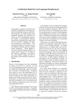
The second scheme simulated two QTLs that determine the differences of
leaf shape among wild-type plants and domesticated plants, respectively. Compared
to the “big” QTL assumed in the first scheme, these two QTLs are “small” because
their two genotypes correspond to slightly different leaf shapes. Figures 4 and 5
provide the results about shape mapping for wild-type plants and domesticated
plants, respectively. In the upper panel (A) of each figure, two original QTL
genotypes are assumed, from which 200 backcross progeny were simulated with a
range of leaf shape. The middle panel (B) gives part of the backcross. In the bottom
panel (C), two genotypes were estimated using our algorithm. It can be seen that
the model can well detect a QTL even if it has a small effect on morphological
shape.
To show the fitness of our model, we put the estimated QTL genotypes on the simu-
lated backcross population forthefirst(A)andsecond(BandC)simulationscheme
(Fig. 6). The leaf shape of t wo QTL genotypes in each case well covers the simulated
leaf shape, showing a good fitness of the mapping model. Also, we calculated the de n-
sity functions for each simulated progeny and two QTL genotypes for each simulation
scheme (Fig. 7). The “big” QTL displays two distinct modes of distribution (Fig. 7A),
whereas there is a small difference in the density functions of two genotypes for each
of two “ small” QTLs (Fig. 7B,C). By comparing Fig. 1A with Fig. 7B and 7C, we can
Figure 3 The first simulation scheme: A “big” QTL controls differences in leaf shape between wild
types and cultivars for cucurbit plants. A: Two given QTL genotypes, QQ for the wild type (left) and Qq
for the cultivar (right); B: Part of the simulated backcross progeny; C: Two estimated QTL genotypes, QQ for
the wild type (left) and Qq for the cultivar (right).
Fu et al. Theoretical Biology and Medical Modelling 2010, 7:28
/>Page 8 of 14
obtain the basic information about how well different QTL genotypes are separated
when QTLs exert different effects on leaf shape.
Discussion

When specific genes that control morphological shape and physiological function are
identified, we are in an excellent position to address fundamental questions related to
growth, development, adaptatio n, domestication, and human health. In the past dec-
ades, the increasing availability of DNA-based markers has inspired our hope to map
genes or quantitative trait loci (QTLs) for complex phenotype s [19-25]. However, only
several studies have been alert to map so-called shape genes; a few successful examples
are the positional cloning of genes for fruit shape in tomato [3,7-9]. These successes
result from the fact that a major mutation occurs to determine shape difference. For
many quantitatively inh erited shape traits, genetic mapping will provide a powerful
tool for characterizing QTLs affecting morphological shape. Klingenberg and collea-
gues [4,5] have developed quantitative genetictheorytoestimatetheheritabilityof
shape by integrating geome tric shape analysis. This theory was used to map s pecific
QTLs for morphometric shapes in the mouse [32,33]. Airey et al. [34] used Procrustes
superimposition to study shape differences in the cortical area map of inbred mice.
In this ar ticle, we present a new statistical model for ma ppin g shape QTLs in a seg-
regating population. The new model embeds shape analysis within a mixture model
framework in which different types of morphological shape are defined for individual
genotypes at a QTL. The model was s olved using a traditional shape correspondence
Figure 4 The second simulation scheme: A “ small” QTL controls differences in leaf shape among
different plants from wild types of cucurbit plants. A: Two given QTL genotypes, QQ for the wild type
(left) and Qq for the cultivar (right); B: Part of the simulated back-cross progeny; C: Two estimated QTL
genotypes, QQ for the wild type (left) and Qq for the cultivar (right).
Fu et al. Theoretical Biology and Medical Modelling 2010, 7:28
/>Page 9 of 14
analysis approach and EM algorithm. The advantage of shape mappin g lies in its
capacity to quantify subtle differences in any corner of a morphological shape and
detect specific QTLs that contribute to these differences. Results from simulation stu-
dies suggest that the model has reasonably high power to detect a QTL that control
shape difference. Even with a modest sample size (200), the model is able to discern
the effect of a QTL with a small effect on morphological shape. The model can be

easily extended to model epistatic interactions on morphological shape by including
more components in the mixture model.
The model will be needed to be modified for integrating developmental events and
their consequences into ontogenetic trajectories of shape. Modern biological studies
display an increasing interest in understanding shape variation in ontogenetic processes
that bring about differentiation at an adult stage [35-37]. In a longitudinal study of
radiographs of the Denver Growth Study, Bulygina et al. [37] investigated the morpho-
logical development of individual difference s in the anterior neurocranium, face, and
basicranium. The modified model can map the QTLs that cause variation in shape
developmental trajectories.
In bi ology, a cell or organ fulfill certain biological functions through its shape. Shape
is thought to govern the extent and pattern of energy, matter and signal transduction
through the surface and inner structure o f the biological object. For this reason, an
understanding of biological curvature and texture has received a surge of interest in
structural biology. The new model can be extended to map the QTLs that determine a
Figure 5 The second simulation scheme: A “ small” QTL controls differences in leaf shape among
different plants from cultivars of cucurbit plants. A: Two given QTL genotypes, QQ for the wild type
(left) and Qq for the cultivar (right); B: Part of the simulated backcross progeny; C: Two estimated QTL
genotypes, QQ for the wild type (left) and Qq for the cultivar (right).
Fu et al. Theoretical Biology and Medical Modelling 2010, 7:28
/>Page 10 of 14
three-dimensional (3D) shape and texture of a biological object. Vision technologies
have been developed to estimate the 3D shape of an object from 2D image data with-
out information about its texture (albedo), its pose and the illumination environment
[38,39]. These technologies include a 3D morphable model (3DMM) that represents
the 3D s hapes and textures as a linear combination of shapes and textures principal
Figure 6 The fitness of estimated QTL genotypes to simulated leaf shape in a backcross. A:A“big”
QTL for the shape difference between wild types and cultivars of cucurbit plants. B:A“small” QTL for the
shape difference between different wild types. C:A“small” QTL for the shape difference between different
cultivars.

Fu et al. Theoretical Biology and Medical Modelling 2010, 7:28
/>Page 11 of 14
components, a stochastic Newton optimization algorithm that ts the 3DMM to a single
facial image, thereby estim ating the 3D shape, the texture and the imaging conditions,
and a multi-features fitting algorithm that uses not only the pixel intensity but also
other image cues such as the edges and the specular highlights. Statistical models can
be developed to map QTLs that control the 3D shape and texture of a biological object
Figure 7 Density f unctions of leaf shape for the simulated backcross (yellow) and two QTL
genotypes. A:A“big” QTL for the shape difference between wild types and cultivars of cucurbit plants. B:
A “small” QTL for the shape difference between different wild types. C:A“small” QTL for the shape
difference between different cultivars.
Fu et al. Theoretical Biology and Medical Modelling 2010, 7:28
/>Page 12 of 14
with image data. A series of hyp othesis tests about the genetic control of topological
features (such as stepness and ridgeness) and texture of a shape will be formulated.
Acknowledgements
NSF/NIH Joint grant DMS/NIGMS-0540745 and the Changjiang Scholars Award to RW. RL’s research is supported by
NIDA, NIH grants R21 DA024260 and R21 DA024266. The content is solely the responsibility of the authors and does
not necessarily represent the official views of the NIDA or the NIH.
Author details
1
Department of Statistics, Pennsylvania State University, University Park, PA 16802, USA.
2
Center for Statistical Genetics,
Pennsylvania State University, Hershey, PA 10733, USA.
3
Center for Computational Biology, Beijing Forestry University,
Beijing 100083, China.
Authors’ contributions
GF derived the model and performed simulation studies. AB, KD, and JL participated in simulation studies. RL

participated in the design of the study. RW conceived of the study, coordinated the design and simulation studies,
and wrote the manuscript. All authors read and approved the final manuscript.
Competing interests
The authors declare that they have no competing interests.
Received: 11 February 2010 Accepted: 1 July 2010 Published: 1 July 2010
References
1. Ricklefs RE, Miles DB: Ecological and evolutionary inferences from morphology: an ecological perspective. Ecological
morphology Univ. of Chicago Press, ChicagoWainwright PC, Reilly SM 1994, 13-41.
2. Reich PB: Body size, geometry, longevity and metabolism: do plant leaves behave like a animal bodies? Trends Ecol
Evol 2001, 16:674-680.
3. Tanksley SD: The genetic, developmental, and molecular bases of fruit size and shape variation in tomato. Plant cell
2004, 16:S181-S189.
4. Klingenberg CP, Leamy LJ: Quantitative genetics of geometric shape in the mouse mandible. Evolution 2001,
55:2342-2352.
5. Klingenberg CP: Quantitative genetics of geometric shape: heritability and the pitfalls of the univariate approach.
Evolution 2001, 57:191-195.
6. Tsukaya H: Leaf shape: genetic controls and environmental factors. Intl J Dev Biol 2005, 49:547-555.
7. Frary A, Nesbitt TC, Grandillo S, Knaap E, Cong B, Liu J, Meller J, Elber R, Alpert KB, Tanksley SD: fw2.2: A quantitative
trait locus key to the evolution of tomato fruit size. Science 2000, 289:85-88.
8. Liu J, Van Eck J, Cong B, Tanksley SD: A new class of regulatory genes underlying the cause of pear-shaped tomato
fruit. Proc Natl Acad Sci USA 2002, 99:13302-13306.
9. Xiao H, Jiang N, Schaffner E, Stockinger EJ, van der Knaap E: A retrotransposonmediated gene duplication underlies
morphological variation in tomato fruit. Science 2008, 319:1527-1530.
10. Bookstein FL: The Measurement of Biological Shape and Shape Change Springer- Verlag, New York 1978.
11. Monteiro LR, Diniz-Filho JA, dos Reis SF, Araujo ED: Geometric estimates of heritability in biological shape. Evolution
2002, 56:563-572.
12. Adams DC, Rohlf FJ, Slice DE: Geometric morphoetrics: ten years of progress following the “revolution”. Ital J Zool
2004, 71:5-16.
13. Bernal B: Size and shape analysis of human molars: Comparing traditional and geometric morphometric
techniques. J Comp Hum Biol 2007, 58:279-296.

14. Stegmann MB, Gomez DD: A Brief Introduction to Statistical Shape Analysis Informatics and Mathematical Modelling,
Technical University of Denmark, DTU 2002.
15. Basri R, Costa L, Geiger D, Jacobs D: Determining the similarity of de- formable shapes. Vision Res 1998, 38:2365-2385.
16. Dempster AP, Laird NM, Rubin DB: Maximum likelihood from incomplete data via the EM algorithm. J Roy Stat Soc
Ser B 1977, 39:1-38.
17. Tsai A, Wells W, Warfield S, Willsky A: An EM algorithm for shape classification based on level sets. Med Image Anal
2005, 9:491-502.
18. Lander ES, Botstein D: Mapping Mendelian factors underlying quantitative traits using RFLP linkage maps. Genetics
1989, 121:185-199.
19. Zeng Z-B: Precision mapping of quantitative trait loci. Genetics 1994, 136:1457-1468.
20. Jansen RC, Stam P: High resolution mapping of quantitative traits into multiple loci via interval mapping. Genetics
1994, 136:1447-1455.
21. Xu S, Atchley W: A random model approach to interval mapping of quantitative trait loci. Genetics 1995,
141:1189-1197.
22. Lynch M, Walsh B: Genetics and Analysis of Quantitative Traits Sinauer Associates, Sunderland, MA 1998.
23. Broman KW, Speed TP: A model selection approach for the identification of quantitative trait loci in experimental
crosses (with discussion). J Roy Stat Soc Ser B 2002, 64:641-656.
24. Zou F, Fine JP, Hu J, Lin DY: An efficient resampling method for assessing genome-wide statistical significance in
mapping quantitative trait loci. Genetics 2004, 168:2307-2316.
25. Yi N, Yandell BS, Churchill GA, Allison DB, Eisen EJ, Pomp D: Bayesian model selection for genome-wide epistatic
quantitative trait loci analysis. Genetics 2005, 170:1333-1344.
Fu et al. Theoretical Biology and Medical Modelling 2010, 7:28
/>Page 13 of 14
26. Ma C-X, Casella G, Wu RL: Functional mapping of quantitative trait loci under-lying the character process: A
theoretical framework. Genetics 2002, 161:1751-1762.
27. Wu RL, Ma C-X, Lou Y-X, Casella G: Molecular dissection of allometry, ontogeny and plasticity: A genomic view of
developmental biology. BioScience 2003, 53:1041-1047.
28. Wu RL, Lin M: Functional mapping How to study the genetic architecture of dynamic complex traits. Nat Rev Genet
2006, 7:229-237.
29. Schlichting CD, Pigliucci M: Phenotypic Evolution: A Norm Reaction Perspective Sinauer Associates, Sunderland, MA 1998.

30. Wu RL, Ma C-X, Casella G: Statistical Genetics of Quantitative Traits: Linkage, Maps, and QTL Springer-Verlag, New York
2007.
31. Dryden IL, Mardia KV: Statistical Shape Analysis John Wiley & Sons, New York 1998.
32. Leamy LJ, Klingenberg CP, Sherratt E, Wolf JB, Cheverud JM: A search for quantitative trait loci exhibiting imprinting
effects on mouse mandible size and shape. Heredity 2008, 101:518-526.
33. Klingenberg CP, Leamy LJ, Cheverud JM: Integration and modularity of quantitative trait locus effects on geometric
shape in the mouse mandible. Genetics 2004, 166:1909-1921.
34. Airey DC, Wu F, Guan M, Collins CE: Geometric morphometrics defines shape differences in the cortical area map of
C57BL/6J and DBA/2J inbred mice. BMC Neurosci 2006, 7:63.
35. Vioarsdottir US, O’Higgins P, Stringer C: A geometric morphometric study of regional differences in the ontogeny of
the modern human facial skeleton. J Anat 2002, 201:211-229.
36. Quillevere F, Debat V, Aurray J-C: Ontogenetic and evolutionary patterns of shape dierentiation during the initial
diversication of paleocene acarininids (planktonic foraminifera). Paleobiology 2002, 28:435-448.
37. Bulygina E, Mitteroecker P, Aiello L: Ontogeny of facial dimorphism and patterns of individual development within
one human population. Am J Phys Anthrop 2006, 131:432-443.
38. Romdhani S, Vetter T: Estimating 3D shape and texture using pixel intensity, edges, specular highlights, texture
constraints and a prior. IEEE Computer Soc Conf Computer Vision Pattern Recog 2005, 2:986-993.
39. Romdhani S, Ho J, Kriegman DJ: Face recognition using 3-D models: Pose and illumination. Proc IEEE 2006,
94:1977-1999.
doi:10.1186/1742-4682-7-28
Cite this article as: Fu et al.: A statistical model for mapping morphological shape. Theoretical Biology and Medical
Modelling 2010 7:28.
Submit your next manuscript to BioMed Central
and take full advantage of:
• Convenient online submission
• Thorough peer review
• No space constraints or color figure charges
• Immediate publication on acceptance
• Inclusion in PubMed, CAS, Scopus and Google Scholar
• Research which is freely available for redistribution

Submit your manuscript at
www.biomedcentral.com/submit
Fu et al. Theoretical Biology and Medical Modelling 2010, 7:28
/>Page 14 of 14