Báo cáo y học: " Identification of biomolecule mass transport and binding rate parameters in living cells by inverse modeling" ppt

BioMed Central
Page 1 of 19
(page number not for citation purposes)
Theoretical Biology and Medical
Modelling
Open Access
Research
Identification of biomolecule mass transport and binding rate
parameters in living cells by inverse modeling
Kouroush Sadegh Zadeh*, Hubert J Montas and Adel Shirmohammadi
Address: Fischell Department of Bioengineering, University of Maryland, College Park, Maryland 20742, USA
Email: Kouroush Sadegh Zadeh* - ; Hubert J Montas - ;
Adel Shirmohammadi -
* Corresponding author
Abstract
Background: Quantification of in-vivo biomolecule mass transport and reaction rate parameters
from experimental data obtained by Fluorescence Recovery after Photobleaching (FRAP) is
becoming more important.
Methods and results: The Osborne-Moré extended version of the Levenberg-Marquardt
optimization algorithm was coupled with the experimental data obtained by the Fluorescence
Recovery after Photobleaching (FRAP) protocol, and the numerical solution of a set of two partial
differential equations governing macromolecule mass transport and reaction in living cells, to
inversely estimate optimized values of the molecular diffusion coefficient and binding rate
parameters of GFP-tagged glucocorticoid receptor. The results indicate that the FRAP protocol
provides enough information to estimate one parameter uniquely using a nonlinear optimization
technique. Coupling FRAP experimental data with the inverse modeling strategy, one can also
uniquely estimate the individual values of the binding rate coefficients if the molecular diffusion
coefficient is known. One can also simultaneously estimate the dissociation rate parameter and
molecular diffusion coefficient given the pseudo-association rate parameter is known. However,
the protocol provides insufficient information for unique simultaneous estimation of three
parameters (diffusion coefficient and binding rate parameters) owing to the high intercorrelation

between the molecular diffusion coefficient and pseudo-association rate parameter. Attempts to
estimate macromolecule mass transport and binding rate parameters simultaneously from FRAP
data result in misleading conclusions regarding concentrations of free macromolecule and bound
complex inside the cell, average binding time per vacant site, average time for diffusion of
macromolecules from one site to the next, and slow or rapid mobility of biomolecules in cells.
Conclusion: To obtain unique values for molecular diffusion coefficient and binding rate
parameters from FRAP data, we propose conducting two FRAP experiments on the same class of
macromolecule and cell. One experiment should be used to measure the molecular diffusion
coefficient independently of binding in an effective diffusion regime and the other should be
conducted in a reaction dominant or reaction-diffusion regime to quantify binding rate parameters.
The method described in this paper is likely to be widely used to estimate in-vivo biomolecule mass
transport and binding rate parameters.
Published: 11 October 2006
Theoretical Biology and Medical Modelling 2006, 3:36 doi:10.1186/1742-4682-3-36
Received: 29 August 2006
Accepted: 11 October 2006
This article is available from: />© 2006 Sadegh Zadeh et al; licensee BioMed Central Ltd.
This is an Open Access article distributed under the terms of the Creative Commons Attribution License ( />),
which permits unrestricted use, distribution, and reproduction in any medium, provided the original work is properly cited.
Theoretical Biology and Medical Modelling 2006, 3:36 />Page 2 of 19
(page number not for citation purposes)
Background
Transport of biomolecules in small systems such as living
cells is a function of diffusion, reactions, catalytic activi-
ties, and advection. Innovative experimental protocols
and mathematical modeling of the dynamics of intracel-
lular biomolecules are key tools for understanding biolog-
ical processes and identifying their relative importance.
One of the most widely used techniques for studying in
vitro and in vivo diffusion and binding reactions, nuclear

protein mobility, solute and biomolecule transport
through cell membranes, lateral diffusion of lipids in cell
membranes, and biomolecule diffusion within the cyto-
plasm and nucleus, is Fluorescence Recovery after Photob-
leaching (FRAP). The technique was developed in the
1970s and was initially used to study lateral diffusion of
lipids through the cell membrane [1-9]. At the time, bio-
physicists paid little attention to the procedure, but since
the invention of the Green Fluorescent Protein (GFP)
technique, also known as GFP fusion protein technology,
and the development of the commercially available con-
focal-microscope-based photobleaching methods, its
applications have increased drastically [10-14]. A detailed
description of the protocol is presented in [13,15].
The number and complexity of quantitative analyses of
the FRAP protocol have increased over the years. Early
analyses characterized diffusion alone [7,16-18]. More
recently, investigators have studied the interaction of GFP-
tagged proteins with binding sites inside living cells
[11,19]. Some have considered faster and slower recovery
as measures of weaker and tighter binding, respectively.
By analyzing the shape of a single FRAP curve, others have
tried to draw conclusions about the underlying biological
processes [12,13,20]. Ignoring diffusion and presuming a
full chemical reaction model, some researchers have per-
formed quantitative analyses to identify pseudo-associa-
tion and dissociation rate coefficients [16,18,20-24].
To describe diffusion-reaction processes in the FRAP pro-
tocol, one needs to solve the full diffusion-reaction
model. Sprague et al. [14] presented an analytical treat-

ment of the diffusion-reaction model and stated where
pure diffusion, pure reaction, and diffusion-reaction
regimes are dominant. They used the model to simulate
the mobility of the GFP-tagged glucocorticoid receptor
(GFP-GR) in nuclei of both normal and ATP-depleted
cells. Using the mass of GFP-GR, they assumed a free
molecular diffusion coefficient of 9.2
µ
m
2
s
-l
for GFP-GR
and fitted two binding rate parameters by curve fitting. On
the basis of these parameters they concluded that GFP-GR
diffuses from one binding site to the next with an average
time of 2.5 ms; the average binding time per site is 12.7
ms. They also concluded that 14% of the GFP-GR is free
and 86% is bound. There have been other theoretical
investigations of full diffusion-reaction models in FRAP
experiments [10,25,26].
What is missing from these comprehensive FRAP analyses
is a robust and systematic method for extracting as much
physiochemical information from the protocol as possi-
ble and for quantifying the related parameters. There are
several in vivo and in vitro methods for measuring mass
transport and reaction rate parameters. However, in vitro
results may not be representative of in vivo transport proc-
esses. In-vivo measurements, on the other hand, often
impose unrealistic and simplified initial and boundary

conditions on transport processes in biological systems.
Also, information regarding parameter uncertainty is not
readily obtained from these methods unless a very large
number of samples and measurements are taken at signif-
icant additional cost [27].
To overcome these limitations, indirect methods such as
parameter optimization by inverse modeling can be used
to identify mass transport and biochemical reaction rate
parameters. Inverse modeling is usually defined as estima-
tion of model parameters by matching a numerical or ana-
lytical model to observed data representing the system
response at a discrete time and location. In other words,
"inverse problems are those where a set of measured
results is analyzed in order to get as much information as
possible on a 'model' which is proposed to represent a sys-
tem in the real world" [28]. Inverse techniques usually
combine a numerical or analytical model with a parame-
ter optimization algorithm and experimental data set to
estimate the optimum values of model parameters,
imposed initial and boundary condition and other prop-
erties of the excitation-response relationship of the system
under study. The technique searches iteratively for the best
combination of parameter values, by varying the
unknown coefficients and comparing the measured
response of the system with the predicted simulation
given by the forward model. The search continues until
the global or local minimum of the objective function,
defined by the differences between the measured and sim-
ulated values of state variable(s), is obtained. Several opti-
mization algorithms have been proposed to solve inverse

problems. They include the steepest descent scheme, con-
jugate gradient method, Newton's algorithm, Gauss-New-
ton method, global optimization technique, Simplex
method, Levenberg-Marquardt algorithm, quasi-Newton
methods, genetic algorithm, and Monte Carlo-Markov
Chain (MCMC) method [28,29].
The task seems straightforward; just a matter of selecting
an appropriate mathematical model and estimating its
parameters via optimization algorithms. However, several
conceptual and computational difficulties have made the
implementation of inverse modeling more challenging:
Theoretical Biology and Medical Modelling 2006, 3:36 />Page 3 of 19
(page number not for citation purposes)
(1) judicious choice of a mathematical model (forward
model) that is representative enough to simulate the
behavior of biological systems, with sufficient accuracy,
and at the same time allows interpretation of the results
beyond pure parameter estimation; (2) the type and qual-
ity of input data is a crucial prerequisite for successful
parameter optimization by inverse modeling. The data
should provide enough information regarding the excita-
tion-response relationship of the system and have reason-
able scatter; (3) well-posedness of the inverse problem,
which depends on the model structure, the quality and
quantity of the input data, and the type of imposed initial
and boundary conditions [27,30].
The goal of this study is to develop, apply, and evaluate a
general purpose inverse modeling strategy for identifying
biomolecule mass transport and binding rate parameters
from the FRAP protocol, studying possible inter-correla-

tions among the parameters, analyzing possible ill-posed-
ness of the inverse problem, and proposing approaches to
obtain unique estimates for biomolecule mass transport
and binding rate parameters. This approach has several
advantages over direct measurement of parameters and
commonly-used model calibration procedures. Unlike
direct methods, inverse modeling does not impose any
constraints on the form or complexity of the forward
model, on the choice of initial and boundary conditions,
on the constitutive relationships, or on the treatment of
heterogeneities via deterministic or stochastic formula-
tions. Therefore, experimental conditions can be chosen
on the basis of convenience rather than by a need to sim-
plify the mathematics of the processes. Additionally, if
information regarding parameter uncertainty and model
accuracy is needed, it can be obtained from the parameter
optimization procedure.
The first section of this paper presents the mathematical
model used to describe diffusion-reaction of biomole-
cules inside cells during the course of the FRAP experi-
ment, along with the numerical algorithm used to solve it
and the approach developed for parameter estimation by
nonlinear optimization. The experimental studies, in
which both a real FRAP experiment and simulations are
considered, are presented in the second section. Results of
parameter estimation for four distinct optimization sce-
narios are presented and discussed in the third section.
This is followed by a possible method for obtaining
unique values for biomolecule mass transport and reac-
tion rate parameters, posedness (stability and unique-

ness) analysis of the inverse problem, and the conclusion
of the study.
Theoretical study
Formulation of the forward problem
Using primary rate kinetics, one can describe the binding
reactions between free biomolecule and vacant binding
sites during the course of the FRAP experiment by
[14,16,26]:
where F is concentration of free biomolecule, S is concen-
tration of vacant binding sites, C is concentration of the
bound complex (C = FS), K
a
is the free biomolecule-
vacant binding site association rate coefficient (T
-1
), and
K
d
is dissociation rate coefficient (T
-1
). The equation only
describes the binding process and assumes uniform distri-
bution of the binding sites. To describe diffusion and reac-
tion of the macro-molecule inside the cell during the
course of the FRAP protocol, one needs to incorporate dif-
fusion in the mathematical model. This can be achieved
by writing a set of three coupled nonlinear partial differ-
ential equations in a cylindrical coordinate system:
in which r is radial coordinate (L) in the cylindrical coor-
dinate system, and D

F
, D
S
, and D
C
are molecular diffusion
coefficients (L
2
T
-1
) for free biomolecules, vacant binding
sites, and bound complex, respectively (symbols L and T
inside parentheses are dimensions).
To develop and solve equation (2) the following assump-
tion were made:
1. The medium is isotropic and homogeneous and the
axes of the diffusion tensors are parallel to those of the
coordinate system. By these assumptions, the second-
order diffusion tensors collapse to the diffusion coeffi-
cients D
F
, D
S
, and D
C
.
2. Two-dimensional diffusion takes place in the plane of
focus. This is a legitimate assumption when the bleaching
area creates a cylindrical path through the cell, which is
the case for a circular bleach spot with reasonable spot

size [14,16]. This assumption eliminates the azimuthal
and vertical components of the coordinate system.
3. There are no advective velocity fields in the bleached
area. We acknowledge that ignoring the convective flux
will lead to the overestimation of the diffusion coefficient,
but in the presence of a binding reaction this overestima-
FS C
K
K
a
d
+
ZXZZ
YZZZ
()1
∂
∂
=
∂
∂
+
∂
∂
+
∂
∂
+
∂
∂
−+

F
t
D
F
r
D
r
F
r
D
r
F
D
F
z
KFS K
Frr Frr F Fzz a
2
22
22
11
θθ
θ
22
dd
Srr Srr Szz a
C
S
t
D

S
r
D
r
S
r
D
r
S
D
S
z
KF
∂
∂
=
∂
∂
+
∂
∂
+
∂
∂
+
∂
∂
−
2
22

22
11
S
θθ
θ
22
SSKC
C
t
D
C
r
D
r
C
r
D
r
F
D
C
d
Crr Crr Czz
+
∂
∂
=
∂
∂
+

∂
∂
+
∂
∂
+
∂
∂
()2
11
2
2
22
C
θθ
θ
22
zz
KFS KC
ad
2
+−
Theoretical Biology and Medical Modelling 2006, 3:36 />Page 4 of 19
(page number not for citation purposes)
tion is negligible. In other words, we assume that the
Peclet number is less than unity and advection is not
dominant.
4. The effects of heating (caused by the absorption of the
laser beam by the sample and fluorophore) on the bio-
molecule mass transport and binding rate parameters are

negligible. In other words, we assume isothermal flow of
biomolecules toward the bleached area from the undis-
turbed region.
5. The diffusion of the bound complex is negligible (D
C
=
0, D
S
= 0).
6. The biological system is in a state of equilibrium before
photobleaching and it remains so over the time course of
the FRAP experiment. This is a reasonable assumption
because most biological FRAP experiments take from sev-
eral seconds to several minutes, whereas the GFP-fusion
expression changes over a time course of hours [14]. This
eliminates the second equation in the system of three cou-
pled nonlinear partial differential equations and hence
Eq. (2) collapses to one site-mobile-immobile model:
Where = K
a
S is the pseudo-association rate coefficient.
System (3) was solved analytically in Laplace space
involving Bessel functions [14] for total fluorescence
recovery averaged over the bleach spot (of radius w). The
solution was adopted from that for a problem of heat con-
duction between two concentric cylinders [31]:
where:
C
eq
+ F

eq
= 1 (8)
In these expressions, s is the Laplace transform variable
that inverts to yield time, (s) is the average of the
Laplace transform of the fluorescent intensity within the
bleach spot, F
eq
and C
eq
are equilibrium concentration of F
and C, and I
1
and K
1
are modified Bessel functions of the
first and second kind.
To obtain (s) as a function of time in real space, one
needs to calculate the inverse Laplace transform numeri-
cally. In the present study, the MATLAB routine invlap.m
[32] was used for this task.
Numerical solution strategy
In this study, the forward model (Eq. 3) is solved using a
fully implicit backward in time and central in space finite
difference approximation. The choice of a numerical
approach was made so that the inversion method could
be readily extended to arbitrary initial and boundary con-
ditions and domain geometry, and especially so that it
could be extended to the system of equations (2) rather
than just its simplified version in (3). The corresponding
discretization of equation (3) is:

Where n is the time step and i denotes location in space.
Rearranging Eq. (9) one obtains the following block tri-
diagonal matrix equation suitable for solution by a linear
algebraic solver:
To solve equation (10) the following initial conditions
were used:
where w is the radius of the bleached area and R is the
length of the spatial domain. The initial condition implies
that the act of bleaching destroys the fluorescence tag on
∂
∂
=
∂
∂
+
∂
∂
−+
∂
∂
=−
()
F
t
D
F
r
D
r
F

r
KF KC
C
t
KF KC
FF ad
ad
2
2
1
3
*
*
K
a
*
frap s
s
F
s
KqwIqw
K
sK
C
sK
eq
a
d
eq
d

() [ ][ ] ( )
*
=− −
()()
+
+
−
+
1
12 1 4
11
q
s
D
K
sK
f
a
d
2
15=+
+
[] ()
*
C
K
KK
eq
a
ad

=
+
*
*
()6
F
K
KK
eq
d
ad
=
+
*
()7
frap
frap
FF
t
D
FFF
r
D
r
FF
i
n
i
n
F

i
n
i
n
i
n
F
i
n
i
n+
+
++
−
+
+
+
−
−
=
−+
()
+
−
1
1
11
1
1
2

1
1
1
2
∆
∆
++
++
+
++
−+
−
=−
()
1
11
1
11
2
9
∆
∆
r
KF KC
CC
t
KF KC
ai
n
di

n
i
n
i
n
ai
n
di
n
*
*
[( )] [ ]
[
*
Dt
rrr
F
Dt
r
KtF
Dt
r
F
i
n
F
ai
n
F
∆

∆∆
∆
∆
∆
∆
∆
1
2
1
1
2
1
1
2
1
−++
()
+−
−
++
(()]
[]
*
1
2
1
1
1
11
11

rr
FKCF
KtC KtF C
i
n
di
n
i
n
di
n
ai
n
i
n
−−=
+−=
+
++
++
∆
∆∆
(()10
Fr
rw
FwrR
Cr
rw
CwrR
eq

eq
0
00
0
00
,
,
,
,
,
,
()
=
<≤
<≤





()
=
<≤
<≤





Theoretical Biology and Medical Modelling 2006, 3:36 />Page 5 of 19

(page number not for citation purposes)
the biomolecules in the bleached area but does not
change the concentrations of free biomolecule, bound
complex, or vacant binding sites. The boundary condi-
tions were formulated as:
which imply that the diffusive biomolecule flux is zero at
the center of the bleach spot and far beyond the bleached
area throughout the course of the FRAP experiment.
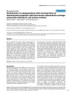
This numerical solution was validated by comparing it to
the analytical solution (4). For this purpose, the average of
the fluorescence intensity within the bleach spot was cal-
culated by [27]:
The results of the comparison for typical parameter values
of D
f
= 1.3
µ
m
2
s
-1
, = 0.01s
-1
, K
d
= 0.25s
-1
, and w = 0.5
µ
m are presented in Figure 1. These results confirm that

the numerical approach used in this study does indeed
produce an accurate solution of Eq. (3).
Formulation of the inverse problem
We want to solve the unconstrained minimization prob-
lem (see Appendix for detailed derivation of equation
(12)):
where r is the residual (differences between the observed
and predicted state variable) column vector, N is the
number of observations, and is only for notational
convenience. Assuming
φ
(p) is twice-continuously differ-
entiable, the gradient vector, ∇
φ
(p), and the Hessian
matrix, ∇
2
φ
(p), of
φ
(p) can be calculated as [33]:
Owing to the nonlinear nature of Eq. (12), its minimiza-
tion was carried out iteratively by first starting with an ini-
tial guess of parameter vector, {p
(k)
} and updating it at
each iteration until the termination criteria were met:
p
(k+1)
= p

(k)
+
α

(k)
∆ p
(k)
(15)
where a
(k)
is a scalar step length and ∆p
(k)
is the direction
of search (step direction).
The linear least square problem below, which avoids the
computation of possibly ill-conditioned J(p
(k)
)
T
J(p
(k)
)
[34,35], was solved to obtain the search direction in each
iteration:
We used QR decomposition [36] to solve Eq. (16).
A combination of "one-sided" and "two-sided" finite dif-
ference methods [37,38] was used to calculate the partial
derivatives of the state variable ( (s)) with respect to
model parameters and to construct the Jacobian matrix:
in each iteration.

∂
∂
=
∂
∂
=
∂
∂
=
∂
∂
=
=→∞
=→∞
F
r
F
r
C
r
C
r
rr
rr
0
0
0
0
frap s
w

rF r C r dr
w
()
=
()
+
()
∫
2
11
2
0
[]()
K
a
*
min ( )
φ
p
()
=
()
=
() ()
=
∑
1
2
1
2

12
2
1
r p rp rp
i
i
N
T
1
2
∇
()
=
()
∂
()
∂
=−
() ()
=
∑
φ
prp
rp
p
Jp rp
i
i
T
i

N
1
1
13()
∇
()
=
∂
()
∂
∂
()
∂
+
∂
()
∂∂
()
=
()
=
∑
2
1
2
φ
p
rp
p
rp

p
rp
pp
rp Jp J
i
j
i
i
i
N
i
ij
i
T
[]pp
rp
pp
rp
i
ij
i
N
i
()
+
∂
()
∂∂
()
=

∑
2
1
14()
min ( )
rp
Jp
D
p
k
k
kk
k
()








+
()
()













0
16
1
2
2
λ
∆
frap
J
rp
p
frap p
p
i
ii
=
∂
()
∂
=−
∂
()
∂

()17
Validation of the numerical model with analytical solutionFigure 1
Validation of the numerical model with analytical solution.
Parameter values D
f
= l.3
µ
m
2
s
-1
, = 0.01s
-1
, K
d
= 0.25 s
-1
,
and w = 0.5
µ
m were used to generate the graph in both
solutions.
K
a
*
Theoretical Biology and Medical Modelling 2006, 3:36 />Page 6 of 19
(page number not for citation purposes)
At the early stages of the optimization, where the search is
far from the solution, the "one-sided" finite difference
scheme, which is computationally cheap, was used [39]:

As the optimization proceeds in descent direction, the
algorithm switches to a more accurate but computation-
ally expensive approach in which the partial derivatives of
(s) with respect to the model parameters are calcu-
lated using a two-sided finite difference scheme:
The switch is made when
φ
(p) ≤ 1 × 10
-2
. A detailed
description of the procedure to update the Jacobian
matrix is presented in [39].
To ensure positive-definiteness of the Hessian matrix and
the descent property of the algorithm, the value of D was
initialized using a p × p identity matrix before the begin-
ning of the optimization process. Then the diagonal ele-
ments were updated in each iteration as follows [27,39];
where j is the j
th
column of the Jacobian matrix and k is the
iteration level in the inverse algorithm. The lines below
were implemented in the algorithm to update D at each
iteration:
for i = 1: p
D(i, i) = max (norm(J(:, i), D(i, i)))
end
In order to update
λ
at each iteration, the optimization
starts with an initial parameter vector and a large

λ
(
λ
= 1).
As long as the objective function decreases in each itera-
tion, the value of
λ
is reduced. Otherwise, it is increased.
The approach avoids calculation of
λ
and step length in
each iteration and is therefore computationally cheap. A
detailed description of the code for updating
λ
is given in
[33].
Finally, to stop the algorithm and to end the search, a
combined termination criterion was used (see [39] for
detailed discussion):
Stop
else
Continue Optimization Loop
end
The developed inverse modeling strategy was then used to
quantify biomolecule mass transport and binding rate
parameters.
Experimental study
To determine the mass transport and binding rate param-
eters of the GFP-tagged glucocorticoid receptor through
the developed inverse modeling strategy, three data sets

were used:
1. A FRAP experiment was conducted on the mouse aden-
ocarcinoma cell line 3617 (McNally, personal communi-
cation), referred to as scenario A. This data set consists of
43 fluorescent recovery values gathered in the course of a
20-second FRAP experiment and post-processed to
remove noise.
2. A generated data set was obtained by solving Eq. (3) for
a hypothetical cell with prescribed initial and boundary
conditions and parameter values: D
f
= 30
µ
m
2
s
-1
, =
30s
-1
, K
d
= 0.1108s
-1
, and w = 0.5
µ
m. The reason for select-
ing these parameter values for data generation and param-
eter optimization is that they represent a situation in
which the Damkohler number is almost unity and neither

of the diffusion and reaction regimes is dominant. Both
these processes are present in the experimental procedure.
The parameter values also imply that the free GFP-GR
molecules are mobile and the bound complex and the
vacant binding sites are relatively immobile (D
C
= 0, D
S
=
0). Predicted FRAP recovery values were sampled at dis-
crete times. The data were corrupted by adding normally
distributed (N(0,0.01)) random error to each "measure-
ment". The synthetic data were then used as input for
parameter optimization problem and posedness analysis
of the inverse problem. The resulting signal and noise are
depicted in Figure 2.
3. The third data set was similar to the second but without
perturbation. The data were used to determine what can
and cannot be identified using FRAP data.
J
frap p p p p p frap p p p p
p
iip ip
=−
+
()
−
()
12 12
, , , , , , ∆

∆
ii
()18
frap
J
frap p p p p p frap p p p p p
iip iip
=−
+
()
−−
12 12
, , , , , , ∆∆
(()
2
19
∆p
i
()
dJ
ddJ
jj
j
i
j
k
j
k
00
1

=
=
−
max( , )
if p
p
p
p
pp
(&&)∇
()
≤×
()
()
≤×
()
≤×
=
−−−
φ
φ
φ
φ
110 110 110
362
∆
K
a
*
Theoretical Biology and Medical Modelling 2006, 3:36 />Page 7 of 19

(page number not for citation purposes)
Four optimization scenarios were considered. In scenario
A, the developed inverse modeling strategy was used to
identify three unknown parameters [D
f
, K
a
, K
d
] for GFP-
GR using the experimental FRAP data. To test the unique-
ness of the model parameters, the optimization algorithm
was carried out using different initial guesses for the
parameter vector (
β
= [D
f
, , K
d
]). In scenario B, two of
the three parameters in one-site-mobile-immobile model
were kept constant and the third was estimated. The goal
was to determine whether or not the FRAP protocol pro-
duces enough information to estimate one parameter
uniquely. The optimization algorithm was used to esti-
mate a single parameter for both noise-free and noisy
data. In scenario C, pairs of model parameters were esti-
mated under the assumption that the value of the third
parameter is known. In the first attempt, the optimized
values of the individual binding rate coefficients were

quantified given a known value for the free molecular dif-
fusion coefficient of the GFP-GR. Again the optimization
algorithm was used for both noise-free and noisy data.
Given the value of the pseudo-association rate, the opti-
mized values of the molecular diffusion coefficient and
dissociation rate coefficient were then estimated. Assum-
ing that the "true" value of the dissociation rate coefficient
is known, we tried to estimate the optimized values of the
free molecular diffusion coefficient and the pseudo-asso-
ciation rate parameter. Again, the goal was to determine
which pairs of parameters, if any, can be estimated
uniquely using FRAP data. Finally, in scenario D, we
investigated the possibility of simultaneous estimation of
three parameters of the one-site-mobile-immobile model
using noise-free FRAP data.
In all the scenarios investigated, the accuracy of the esti-
mation was quantified by calculating and analyzing good-
ness-of-fit indices such Root Mean Squared Error (RMSE)
and the Coefficient of Determination (R
2
). The root mean
squared error and coefficient of determination were calcu-
lated as follows [27,40,41]:
RMSE = (r
T
r/(N - p))
1/2
(20)
where U
i

and
i
are the observed and predicted state var-
iable ( (s)), respectively.
Results and discussion
Scenario A: Simultaneous identification of transport and
binding rate parameters
In this scenario, the aim was to estimate the transport and
binding rate parameters for GFP-GR simultaneously by
coupling the experimental data from the FRAP protocol,
the Levenberg-Marquardt algorithm, and the numerical
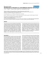
solution of Eq. (3). The results are given in Table 1 and
Figure 3.
Analysis of Table 1 reveals several points regarding the
mobility and binding of GFP-GR inside the nucleus. First,
as pointed out in [14], the primary rate kinetics or single-
binding state (Eq. 1) can satisfactorily describe the bind-
ing process of GFP-GR inside the nucleus. Therefore, we
did not attempt to develop a two-site-mobile-immobile
model to simulate the mobility and binding of GFP-GR.
Second, the values for mass transport and binding rate
parameters estimated in [14] are given as run 20 in Table
1 and Figure 3 for sake of comparison. Table 1 and Figure
3 indicate many combinations of three parameters that
give essentially the same error level (or objective function
magnitude) and produce equally excellent fits (only 20
runs were reported). The values obtained in [14] represent
only one of the possible solutions. In other words, the
inverse problem is not well-posed and has no unique
solution. This explains the conflicting parameter values

that have been reported by investigators for a special bio-
molecule using the FRAP protocol. The reason for the ill-
posedness of the inverse problem is that the FRAP proto-
K
a
*
R
UU U U
UUUU
ii i i
ii
2
2
2
22 2
21=
−
−−
∑∑∑
∑∑ ∑∑
[]
[ ( )][ ( )]
()
ˆ
U
frap
The generated noise free and noisy signals for FRAP protocolFigure 2
The generated noise free and noisy signals for FRAP proto-
col. The signal was generated by solving Eq. (3) for a hypo-
thetical cell with prescribed initial and boundary conditions

and parameter values: D
f
= 30
µ
m
2
s
-1
, = 30 s
-1
, K
d
=
0.1108 s
-1
, and w = 0.5
µ
m.
K
a
*
Theoretical Biology and Medical Modelling 2006, 3:36 />Page 8 of 19
(page number not for citation purposes)
col, though useful for studying the dynamics of cells, pro-
vides insufficient information to estimate mass transport
and binding rate parameters of biomolecules uniquely
and simultaneously.
Third, the optimized values of the free molecular diffu-
sion coefficient for GFP-GR range from 1.2 to 79.7179
µ

m
2
s
-1
. Except for D
f
= 79.1719
µ
m
2
s
-1
the estimated val-
ues are physically reasonable. Note that we did not take
into account the convective flux of GFP-GR toward the
bleached area (in equations 2 and 3), which means that
the optimized values of the molecular diffusion coeffi-
cient are somewhat overestimated in comparison to the
"true" value.
Fourth, using Eqs. (6) and (7), Sprague et al. [14] con-
cluded that 86% of the GFP-GR is bound and only 14% is
free. Our study, however, indicates that using FRAP, one
cannot say how much of the biomolecule is free and how
much is bound. As Table 1 shows, the concentration of
free GFP-GR ranges from zero to 100%. The same is true
for the concentration of the bound complex. For instance,
referring to the results obtained in run 9, one may con-
clude that 100% of the GFP-GR is free, while the results of
run 10 show that all of it is bound. Note that both these
runs produce excellent fits with the same RMSE and coef-

ficient of determination (see Figure 3: scenarios 9 and 10).
Fifth, the average binding time per vacant site, calculated
by t
b
= 1/K
d
[14], varies between 0.72 ms and 4.016 s.
Again this shows that the findings of [14], that the average
binding time per vacant site for GFP-GR is 12.7 ms, repre-
sent just one the possible values. Similarly, the average
time for diffusion of GFP-GR from one binding site to the
next, obtained by t
d
= 1/ [42], ranges between 0.4 ms to
34.3 hours (1.2345*10
5
s). The broad range of t
d
for GFP-
GR indicates that it is meaningless to give an average time
for macro-molecule diffusion inside living cells.
Overall, these results indicate that using experimental
data from the FRAP protocol and coupling it with curve
fitting methods, one cannot draw conclusions regarding
binding reaction, slow or rapid mobility of biomolecules,
and concentrations of free macromolecule, vacant bind-
ing sites and bound complex inside living cells. The results
of parameter estimation should be coupled with other
experimental studies and large scale optimization tech-
niques such as Monte-Carlo simulation to prevent mis-

leading conclusions and inferences.
Scenario B: Estimation of a single parameter in a FRAP
experiment
In this scenario, two of the three parameters were kept at
their "true" values and the optimized value of the third
parameter was estimated. The optimization algorithm was
K
a
*
Table 1: The results of optimization for scenario A.
Initial guesses Optimized values
run D
f
(
µ
m
2
s
-1
)
(s
-1
)
K
d
(s
-1
) D
f
(

µ
m
2
s
-1
)
(s
-1
)
K
d
(s
-1
) F
eq
C
eq
t
b
(ms) t
d
(ms) RMSE R
2
1 1.4 0.01 0.24 1.3454 0.0081 0.249 0.9685 0.0315 4016 123450 0.0241 0.9904
2 15 500 86 13.5563 806 83 0.0934 0.9066 12.00 1.2407 0.0233 0.9912
3 10 20 50 1.2689 22.88 538 0.9592 0.0408 1.90 44.00 0.0245 0.9903
4 1.26 3000 5 79.7179 1.06*10
4
168 0.0156 0.9844 6.00 9.00 0.0236 0.9910
5 12 30 490 1.8558 256 489 0.6564 0.3436 2.00 3.91 0.0244 0.9904

6 1.2 200 49 7.4289 200 42.5 0.1753 0.8247 23.50 5.00 0.0235 0.9911
7 7 2 470 1.2248 4.70 540.72 0.9914 0.0086 1.80 213.00 0.0245 0.993
8 0.7 202 0.047 6.6616 56.362 38.25 0.4043 0.5957 26.10 18.00 0.0235 0.9910
9 1.5 0.001 85 1.2127 7*10
-5
91.21 1.000 0.000 11.00 15.00 0.0246 0.9902
10 1.5 0.1 1*10
-5
1.2127 0.1874 1*10
-5
0.0001 0.9999 200 5336 0.0245 0.9903
11 1.5 1*10
-5
1 1.4652 0.1974 2.1902 0.9173 0.0827 456.6 5066 0.0251 0.9900
12 9.2 500 86.4 8.3315 468.56 83.38 0.1511 0.8489 12.00 2.00 0.0234 0.9911
13 25 0.001 100 1.2534 1.3557 44.94 0.9707 0.0293 22.30 738 0.0245 0.9903
14 0.25 0.001 100 1.2236 0.4235 119.71 0.9965 0.0035 8.40 2361 0.0245 0.9903
15 5 400 0.40 10.1911 396.8 56.7 0.1250 0.8750 17.60 2.52 0.0233 0.9911
16 15 4 1400 1.2205 3.81 1389 0.9973 0.0027 7.00 262 0.0245 0.9903
17 4.5 150 385 4.3970 986 380 0.2782 0.7218 2.60 1.00 0.0242 0.9905
18 10 150 385 8.861 2458 396 0.1388 0.8612 2.50 0.40 0.0242 0.9905
19 0.4 0.5 0.003 1.6371 0.5211 3.20 0.86 0.1400 312.50 1919 0.0254 0.9901
20
#
- - - 9.20 500 86.4 0.1474 0.8526 11.60 2.00 0.0255 0.9886
# These values were obtained by Sprague et al. [14].
K
a
*
K

a
*
Theoretical Biology and Medical Modelling 2006, 3:36 />Page 9 of 19
(page number not for citation purposes)
Predicted and experimental FRAP recovery curves for GFP-GR using one-site-mobile-immobile model (dots: Observed, solid lines: Simulated)Figure 3
Predicted and experimental FRAP recovery curves for GFP-GR using one-site-mobile-immobile model (dots: Observed, solid
lines: Simulated). Experimental data are from McNally (personal communication).
Theoretical Biology and Medical Modelling 2006, 3:36 />Page 10 of 19
(page number not for citation purposes)
used to estimate a single parameter for both noise-free
and noisy data and the results are presented in Tables 2, 3,
4. The values inside parentheses are for noisy data. As
these tables show, the FRAP protocol provides enough
information to estimate one parameter uniquely if the
other two are known. This is true for both noise-free and
noisy data. The other important finding is the robustness
and efficiency of the developed optimization algorithm,
which converged to the "true" values of the parameters
regardless of the initial guesses (compare the initial
guesses for the parameters with the optimized values).
Scenario C: Estimation of two parameters in a FRAP
experiment
In this scenario, the optimized values of the binding rate
coefficients were first estimated given that the "true" value
of the molecular diffusion coefficient of GFP-GR was
known. Again, the optimization algorithm was used for
both noise-free and noisy data and the results are given in
Table 5. As Table 5 indicates, using the FRAP experiment
coupled with the proposed inverse modeling strategy, one
can estimate the individual values (not just the ratio) of

the binding rate coefficients uniquely if the value of the
diffusion coefficient is known. This is true for both noise-
free and noisy data.
We then tried to identify the optimized values of the
molecular diffusion coefficient and dissociation rate coef-
ficient for both noise-free and noisy data given that is
known. The results are presented in Table 6, which indi-
cates that the FRAP protocol provides enough informa-
tion to estimate the molecular diffusion coefficient and
dissociation rate parameter uniquely for both noise-free
and noisy data.
Finally, we tried to estimate the optimized values of the
free molecular diffusion coefficient and pseudo-associa-
tion rate parameter by fixing K
d
at the "true" value for both
noise-free and noisy data. The results are shown in Table
7. This table indicates that the FRAP experiment provides
insufficient information for unique simultaneous estima-
tion of the molecular diffusion coefficient and the
pseudo-association rate parameter even for noise-free
data. One must know one of them and try to estimate the
other from the FRAP data using the inverse modeling
strategy.
It can be argued that the reason for the non-uniqueness of
the inverse problem lies in the relationship between the
free molecular diffusion coefficient and the pseudo-asso-
ciation rate parameter. To investigate the possibility of
high intercorrelation between these two parameters fur-
ther, the parameter covariance matrix was calculated [37]:

K
a
*
CsJJ
e
T
=
()
−
2
1
22()
Table 2: The results of parameter optimization for scenario B (estimation of molecular diffusion coefficient in a FRAP experiment).
Estimate D
f
Initial guesses Optimized values
D
f
(
µ
m
2
s
-1
)
(s
-1
)
K
d

(s
-1
) D
f
(
µ
m
2
s
-1
)
(s
-1
)
K
d
(s
-1
) RMSE R
2
3 30 0.1108 29.9975
(29.8032)
30 0.1108 0.00 (0.01) 1.0000 (0.9984)
5 30 0.1108 29.9968
(29.7362)
30 0.1108 0.00 (0.01) 1.0000 (0.9984)
10 30 0.1108 29.9968
(29.7978)
30 0.1108 0.00 (0.01) 1.0000 (0.9984)
15 30 0.1108 29.9959

(29.7483)
30 0.1108 0.00 (0.01) 1.0000 (0.9984)
20 30 0.1108 29.9972
(29.7490)
30 0.1108 0.00 (0.01) 1.0000 (0.9984)
45 30 0.1108 29.9974
(29.7376)
30 0.1108 0.00 (0.01) 1.0000 (0.9984)
1000 30 0.1108 29.9973
(29.7507)
30 0.1108 0.00 (0.01) 1.0000 (0.9984)
500 30 0.1108 29.9969
(29.7910)
30 0.1108 0.00 (0.01) 1.0000 (0.9984)
The values in parentheses were obtained using corrupted data.
K
a
*
K
a
*
Theoretical Biology and Medical Modelling 2006, 3:36 />Page 11 of 19
(page number not for citation purposes)
where C is the first-order approximation of the parameter
covariance matrix, J is the final optimized Jacobian
matrix, which can easily be obtained at the end of optimi-
zation, and s
e
is the estimated error variance [27]:
s

e
= r
T
r/(N - p) (23)
The diagonal elements of the parameter covariance matrix
are variances and the off-diagonal elements are the covar-
iances between the parameters. Using this matrix, one can
calculate the parameter correlation matrix (also known as
the variance-covariance matrix), which is a square matrix
[27]:
COR (P)
ij
= C
ij
/[(C
ii
)
1/2
(C
jj
)
1/2
] (24)
Equation (24) identifies the degree of linear correlation
between the optimized parameters. In other words, the
correlation matrix quantifies the nonorthogonality
between two parameters. A value of ± 1 reflects perfect lin-
ear correlation between two parameters whereas 0 indi-
cates no correlation at all. The matrix may be used to
identify which parameter, if any, is kept constant in the

parameter optimization process because of high intercor-
relation [41]. The correlation matrix for scenario C was
found to be:
COR P
()
=
−
−
−−
1 0000 0 9890 0 2487
0 9890 1 0000 0 1196
0 2487 0 119
.
.
66 1 0000.










Table 4: The results of parameter optimization for scenario B (estimation of dissociation rate coefficient in a FRAP experiment).
Estimate K
d
Initial guesses Optimized values
D

f
(
µ
m
2
s
-1
)
(s
-1
)
K
d
(s
-1
) D
f
(
µ
m
2
s
-1
)
(s
-1
)
K
d
(s

-1
) RMSE R
2
30 30 0.0008 30 30 0.1108 (0.1107) 0.0000 (0.0102) 1.000 (0.998)
30 300 0.8000 30 30 0.1108 (0.1107) 0.0000 (0.0102) 1.000 (0.998)
30 30 0.0001 30 30 0.1108 (0.1107) 0.0000 (0.0102) 1.000 (0.998)
30 30 1.0000 30 30 0.1108 (0.1107) 0.0000 (0.0102) 1.000 (0.998)
30 30 0.0500 30 30 0.1108 (0.1107) 0.0000 (0.0102) 1.000 (0.998)
30 30 0.0010 30 30 0.1108 (0.1107) 0.0000 (0.0102) 1.000 (0.998)
30 30 1 × 10
-5
30 30 0.1108 (0.1108) 0.0000 (0.0102) 1.000 (0.998)
30 30 1 × 10
-6
30 30 0.1108 (0.1107) 0.0000 (0.0102) 1.000 (0.998)
The values in parentheses were obtained using corrupted data.
K
a
*
K
a
*
Table 3: The results of parameter optimization for scenario B (estimation of pseudo-association rate coefficient in a FRAP
experiment).
Estimate
Initial guesses Optimized values
D
f
(
µ

m
2
s
-1
)
(s
-1
)
K
d
(s
-1
) D
f
(
µ
m
2
s
-1
)
(s
-1
)
K
d
(s
-1
) RMSE R
2

30 3.00 0.1108 30 30.0032 (30.3523) 0.1108 0.00 (0.01) 1.000 (0.998)
30 1 × 10
-3
0.1108 30 29.9982 (30.2455) 0.1108 0.00 (0.01) 1.000 (0.998)
30 1 × 10
-6
0.1108 30 30.0031 (30.2468) 0.1108 0.00 (0.01) 1.000 (0.998)
30 1 × 10
6
0.1108 30 30.0030 (30.2478) 0.1108 0.00 (0.01) 1.000 (0.998)
30 1 × 10
3
0.1108 30 30.0031 (30.2507) 0.1108 0.00 (0.01) 1.000 (0.998)
30 300.00 0.1108 30 30.0030 (30.3188) 0.1108 0.00 (0.01) 1.000 (0.998)
30 10.00 0.1108 30 30.0030 (30.2115) 0.1108 0.00 (0.01) 1.000 (0.998)
30 0.050 0.1108 30 30.0030 (30.1655) 0.1108 0.00 (0.01) 1.000 (0.998)
The values in parentheses were obtained using corrupted data.
K
a
*
K
a
*
K
a
*
Theoretical Biology and Medical Modelling 2006, 3:36 />Page 12 of 19
(page number not for citation purposes)
where the diagonal elements of the matrix are the correla-
tions of each parameter with itself (i.e. unity).

The correlation between the molecular diffusion coeffi-
cient and the pseudo-association rate parameter is
= 0.989, and those between the molecular diffusion coef-
ficient-dissociation rate parameter and reaction rate coef-
ficients are = -0.2487 and = -0.1196,
respectively. The signs of the elements of the correlation
matrix are physically reasonable because on the basis of
the primary rate kinetics, Eq. (1), we expect a negative cor-
relation between D
f
and K
d
as well as between K
a
and K
d
.
We also expect a positive correlation between K
a
and D
f
.
The high intercorrelation between the molecular diffusion
coefficient and the pseudo-association rate coefficient
makes it impossible to obtain a unique solution for the
inverse problem using experimental data from the FRAP
protocol. The common practice in these situations is to fix
one parameter and estimate the other by parameter opti-
mization algorithms.
Scenario D: Estimation of three parameters for noise-free

FRAP data
In this scenario we tried to estimate the optimized values
of the mass transport and binding rate coefficients for
noise-free data. As Table 8 indicates, the FRAP experiment
provides insufficient information for unique simultane-
ous estimation of the mass transport and binding rate
parameters even for noise-free data. The reason, as dis-
cussed above, is the high intercorrelation between the
r
DK
fa
−
*
r
DK
fd
−
r
KK
ad
*
−
Table 5: The results of parameter optimization for scenario C (estimation of two parameters in a FRAP experiment: - K
d
).
Estimate K
a
and K
d
Initial guesses Optimized values

D
f
(
µ
m
2
s
-1
)
(s
-1
)
K
d
(s
-1
) D
f
(
µ
m
2
s
-1
)
(s
-1
)
K
d

(s
-1
) RMSE R
2
30 90 0.005 30 30.0246 (32.7366) 0.1108 (0.1122) 0.00 (0.01) 1.000 (0.99)
30 20 0.01 30 29.9762 (28.8955) 0.1108 (0.1101) 0.00 (0.01) 1.000 (0.99)
30 250 0.01 30 30.0729 (33.7009) 0.1108 (0.1128) 0.00 (0.01) 1.000 (0.99)
30 435 0.0005 30 30.1108 (34.2443) 0.1108 (0.1131) 0.00 (0.01) 1.000 (0.99)
30 10 0.01 30 29.9576 (31.8386) 0.1108 (0.1118) 0.00 (0.01) 1.000 (0.99)
30 100 1 30 30.0027 (36.0428) 0.1108 (0.1141) 0.00 (0.01) 1.000 (0.99)
30 100 2*10
6
30 30.0209 (33.8034) 0.1108 (0.1129) 0.00 (0.01) 1.000 (0.99)
30 1000 0.5 30 30.0082 (32.7609) 0.1108 (0.1122) 0.00 (0.01) 1.000 (0.99)
The values in parentheses were obtained using corrupted data.
K
a
*
K
a
*
K
a
*
Table 6: The results of parameter optimization for scenario C (estimation of two parameters in a FRAP experiment: D
f
- K
d
).
Estimate D

f
and K
d
Initial guesses Optimized values
D
f
(
µ
m
2
s
-1
)
(s
-1
)
K
d
(s
-1
) D
f
(
µ
m
2
s
-1
)
(s

-1
)
K
d
(s
-1
) RMSE R
2
8 30 0.008 30.0111 (27.528) 30 0.1108 (0.1122) 0.000 (0.0101) 1.000 (0.998)
48 30 0.08 29.9972 (29.935) 30 0.1108 (0.1108) 0.000 (0.0101) 1.000 (0.998)
8 30 1 29.9989 (28.204) 30 0.1108 (0.1118) 0.000 (0.0101) 1.000 (0.998)
80 30 1 30.0100 (28.294) 30 0.1108 (0.1117) 0.000 (0.0101) 1.000 (0.998)
150 30 0.01 30.0156 (36.477) 30 0.1108 (0.1077) 0.000 (0.0104) 1.000 (0.998)
0.150 30 0.1 30.0005 (27.822) 30 0.1108 (0.1120) 0.000 (0.0101) 1.000 (0.998)
15 30 0.001 30.0090 (24.555) 30 0.1108 (0.1143) 0.000 (0.0102) 1.000 (0.998)
150 30 0.001 30.0142 (188.225) 30 0.1108 (0.0946) 0.000 (0.0133) 1.000 (0.998)
The values in parentheses were obtained using corrupted data.
K
a
*
K
a
*
Theoretical Biology and Medical Modelling 2006, 3:36 />Page 13 of 19
(page number not for citation purposes)
molecular diffusion coefficient and the pseudo-associa-
tion rate parameter.
Unique parameter identification
The optimization scenarios considered above show a pos-
sible way of obtaining unique values for diffusion coeffi-

cient and binding rate parameters of biomolecules inside
living cells. A possible procedure for obtaining unique
values for molecular diffusion coefficient and reaction
rate parameters of macro-molecules is to conduct two
FRAP experiments in different regimes on the same class
of cell and biomolecule. One experiment should be con-
ducted in an effective diffusion regime to estimate diffu-
sion coefficient independent of binding. The other should
be performed in reaction dominant or diffusion-reaction
dominant regimes to identify the binding rate parameters.
Conducting two FRAP experiments in two different
regimes is, however, beyond the scope of the present
study. It will be pursued in future research.
Posedness analysis of the inverse problem
To study the non-uniqueness problem from another
angle, we performed a posedness analysis of the inverse
problem. A problem is ill-posed when it either has no
solution at all, or no unique solution, or the solution is
not stable [43]. Generally, ill-posedness in an inverse
problem arises from non-uniqueness and instability. To
investigate the ill-posedness of the inverse problem, we
analyzed both its stability and its uniqueness.
Stability analysis
Instability occurs when the estimated parameters are
excessively sensitive to the input data. Any small errors in
measurements will then lead to significant error in esti-
mated values of parameters [27]. To perform the stability
analysis, the data sets were corrupted by adding N(0,
σ
2

)
noise to each measurement. The resulting noisy data were
then used as input for parameter optimization algorithm.
The results are given in Tables 2 to 7 in parentheses. As
these tables show, small changes in the input data gener-
ate no significant changes in the optimized values of the
parameters. Therefore, the cause of the ill-posedness of
the inverse problem is not instability.
Uniqueness analysis
Non-uniqueness occurs when multiple parameter vectors
can produce almost the same values of the objective func-
tion, thus making it impossible to obtain a unique solu-
tion [27]. This problem is closely related to parameter
identifiability. In other words, is it possible to obtain
accurate values for parameters in the mathematical model
from the available experimental data? Parameter identifi-
ability depends on both the structure of the mathematical
model and the experimental data used. A common cause
for non-identifiability of model parameters is, as noted in
previous section, high intercorrelation among parameters.
In these situations a change in one parameter generates a
corresponding change in the correlated parameter making
it impossible to obtain accurate estimates of either. Fur-
Table 7: The results of parameter optimization for scenario C (estimation of two parameters in a FRAP experiment: D
f
- ).
Estimate D
f
and
Initial guesses Optimized values

D
f
(
µ
m
2
s
-1
)
(s
-1
)
K
d
(s
-1
) D
f
(
µ
m
2
s
-1
)
(s
-1
)
K
d

(s
-1
) RMSE R
2
50 3 0.1108 3.8162 (6.9081) 4.1352 (7.2953) 0.1108 0.0042 (0.0104) 0.9997 (0.9983)
3 50 0.1108 47.7952
(35.6424)
47.5709
(35.8541)
0.1108 0.0003 (0.0102) 1.0000 (0.9984)
20 25 0.1108 25.2109
(25.2109)
25.2769
(25.2769)
0.1108 0.0001 (0.0001) 1.0000 (1.0000)
25 20 0.1108 24.5737
(24.5737)
24.6488
(24.6488)
0.1108 0.0002 (0.0002) 1.0000 (1.0000)
28 35 0.1108 34.8874
(34.8874)
34.8255
(34.8255)
0.1108 0.0001 (0.0001) 1.0000 (1.0000)
0.1 100 0.1108 89.9205
(89.9205)
89.1097
(89.1097)
0.1108 0.0005 (0.0005) 1.0000 (1.0000)

100 0.1 0.1108 8.5511 (8.5511) 8.8336 (8.8336) 0.1108 0.0017 (0.0017) 1.0000 (1.0000)
28 28 0.1108 28.2015
(28.2015)
28.2282
(28.2282)
0.1108 0.0001 (0.0001) 1.0000 (1.0000)
The values in parentheses were obtained using corrupted data.
K
a
*
K
a
*
K
a
*
K
a
*
Theoretical Biology and Medical Modelling 2006, 3:36 />Page 14 of 19
(page number not for citation purposes)
thermore, even when parameters in a mathematical
model are independent of each other, the experimental
data may produce an objective function that is not sensi-
tive enough to one or more parameters. The characteristic
of the second situation is wide confidence regions on the
estimated parameters and large estimation variances.
Whereas the only solution for the first case is to fix one of
the parameters and estimating the other, performing
multi-objective optimization or conducting different

experiments in which different state variables are meas-
ured may lead to a unique solution in the second case.
To investigate the non-uniqueness of the inverse problem
further, the two-dimensional parameter response surfaces
were constructed and analyzed:
Two-dimensional parameter response surfaces
The uniqueness of the inverse problem was evaluated by
constructing two-dimensional parameter response sur-
faces of the objective function, Φ( ), as a function of
pairs of parameters being optimized. The objective func-
tion was calculated for three parameter planes: D
f
- ,
D
f
- K
d
, and - K
d
. The response surfaces were calculated
using a rectangular grid. The domain of each parameter
was discretized into 100 discrete points resulting in 10000
grid points for each response surface plot.
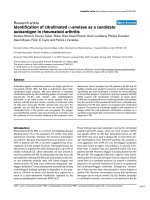
Figures 4a, 4b, 4c, and 4d present response surface plots
of the objective function Φ( ). The D
f
- plane in
Figure 4a indicates a well-defined valley, which starts at
low values of both parameters and extends linearly to the
entire parameter domain. Figure 4a clearly shows a linear

relationship between the molecular diffusion coefficient
and the pseudo-association rate coefficient, which con-
firms the high intercorrelation between them, and there-
fore indicates the difficulty in finding unique values for
them. Indeed, an infinite number of combinations of the
parameters D
f
and (inside the valley) can give almost
the same objective function value and produce an excel-
lent fit. This can be confirmed by a slice of three-dimen-
sional parameter hyper-space in the D
f
- - K
d
directions
(K
on
and K
off
were used for and K
d
in the graph, respec-
tively) presented in Figure 4d (the plot is scaled logarith-
mically). Note that the value of K
d
is fixed on the known
value (0.1108s
-1
). The dark blue area on the slice has the
same error level (objective function) indicating that any

combination of D
f
and on this region will produce the
same error and hence the inverse problem is ill-posed.
Both Figures show a strong linear positive correlation
between D
f
and confirming the result of the parameter
variance-covariance matrix.
The contours of the objective function in D
f
- K
d
and -
K
d
planes are presented in Figures 4b and 4c. Figure 4b
indicates that for small values of the dissociation rate coef-
ficient, the objective function is not sensitive to the molec-
ular diffusion coefficient, which yields an elongated valley
in the D
f
direction. As K
d
increases the objective function
becomes sensitive to the changes in the free molecular dif-
fusion coefficient, which makes it possible to identify this
parameter. For large values of K
d
, the objective function

frap
K
a
*
K
a
*
frap
K
a
*
K
a
*
K
a
*
K
a
*
K
a
*
K
a
*
K
a
*
Table 8: The results of parameter optimization for scenario D (estimation of three parameters for noise-free FRAP data).

Estimate D
f
, K
d
, and
Initial guesses Optimized values
D
f
(
µ
m
2
s
-1
)
(s
-1
)
K
d
(s
-1
) D
f
(
µ
m
2
s
-1

)
(s
-1
)
K
d
(s
-1
) RMSE R
2
20 43 0.01 41.8564 42.7664 0.1112 0.0002 1.0000
200 43 0.01 170.9403 166.9715 0.1106 0.0006 1.0000
27 28 0.01 27.7434 27.6444 0.1107 0.0001 1.0000
29 29 0.01 29.0008 29.0018 0.1108 0.0000 1.0000
29 29 0.001 21.8680 21.5410 0.1104 0.0002 1.0000
29 290 0.0001 276.5849 287.3558 0.1117 0.0005 1.0000
15 500 0.0001 462.2080 491.3985 0.1121 0.0005 1.0000
15 0.5 0.8 3.65890 3.6106 0.1087 0.0043 0.9997
The values in parentheses were obtained using corrupted data.
K
a
*
K
a
*
K
a
*
Theoretical Biology and Medical Modelling 2006, 3:36 />Page 15 of 19
(page number not for citation purposes)

becomes insensitive to the dissociation rate coefficient,
which produces an elongated valley in the K
d
direction. In
a small region where the objective function is sensitive to
both parameters, it is possible to identify both parame-
ters. Parameter optimization in this zone will produce
small estimation variance and narrow confidence inter-
vals.
The contours of the objective function in - K
d
plane
(Figure 4c) shows that the objective function is not sensi-
tive to the pseudo-association rate coefficient when
increases but becomes more sensitive to this parameter
when decreases. In very low values of the dissociation
rate coefficient, the objective function becomes less sensi-
tive to K
d
. When both parameters are small, there are good
chances to identify them with less uncertainty.
Figure 4a shows several apparent local minima when both
the free molecular diffusion coefficient and the pseudo-
association rate parameter are small. To investigate the
K
a
*
K
a
*

K
a
*
Contours of the objective function, Φ(), in a) D
f
- , b) D
f
- K
d
, c) - K
d
, and d) D
f
- - K
d
planes for the synthetic
data
Figure 4
Contours of the objective function, Φ(), in a) D
f
- , b) D
f
- K
d
, c) - K
d
, and d) D
f
- - K
d

planes for the synthetic
data. The response surfaces were generated using a rectangular grid. The domain of each parameter was discretized into 100
discrete points resulting in 10000 grid points for each response surface plot.
a
b
d
c
frap
K
a
*
K
a
*
K
a
*
frap
K
a
*
K
a
*
K
a
*
Theoretical Biology and Medical Modelling 2006, 3:36 />Page 16 of 19
(page number not for citation purposes)
possibility of obtaining a local minimum for inverse

problem further when the model parameters are small,
one of the possible solutions (D
f
= 3
µ
m
2
s
-1
, = 0.03s
-1
,
and K
d
= 0.1824s
-1
) was used to construct response sur-
faces. The results are depicted in Figures 5a, 5b, and 5c. As
these figures show, there are good possibilities for finding
a local minimum in lower subspace of parameters. This is
in contrast with the findings of [14], which reported very
high values ( = 500s
-1
, K
d
= 86.4s
-1
) for these parame-
ters (See run 20 in Table 1).
The important findings from the analysis of the two-

dimensional parameter response surfaces can be summa-
rized as:
First, response surfaces, though very useful in analyzing
the identifiability of the parameters being optimized, are
only two-dimensional cross-sections of a full p – dimen-
sional parameter hyper-space. The bound response surface
K
a
*
K
a
*
Contours of the objective function, Φ( ), in a) D
f
- , b) D
f
- K
d
, and c) - K
d
planes for GFP-GR (Scenario A) in lower
subspace of model parameters
Figure 5
Contours of the objective function, Φ( ), in a) D
f
- , b) D
f
- K
d
, and c) - K

d
planes for GFP-GR (Scenario A) in lower
subspace of model parameters. The response surfaces were generated using a rectangular grid. The domain of each parameter
was discretized into 100 discrete points resulting in 10000 grid points for each response surface plot. Intensity scale is the
same as Figure 4.
c
ba
frap
K
a
*
K
a
*
frap
K
a
*
K
a
*
Theoretical Biology and Medical Modelling 2006, 3:36 />Page 17 of 19
(page number not for citation purposes)
does not automatically guarantee a unique solution for
the inverse problem. Other local minima or even a global
minimum may exist in different regions of the parameter
space that do not show up in the response surfaces. Even
a well-defined minimum in one part of a two-dimen-
sional plane does not automatically guarantee that no
other minima exist and that the inverse problem is

unique.
Second, the behavior of the objective function varies
between different sub-spaces of the parameter domain.
The D
f
- and D
f
- K
d
planes, for instance, are almost
mirror images of each other in the lower space of the
parameter domain while in the upper subspace of the
parameter domain the D
f
- plane shows a strong pos-
itive linear relationship.
Third, several small local minima in the two-dimensional
plane may be produced by minor oscillations of the
numerical simulator. Care should be exercised in inter-
preting these minima.
Conclusion
The following results can be drawn from this study:
1. The FRAP protocol provides enough information to
estimate one parameter uniquely.
2. Coupling experimental FRAP data with the parameter
optimization methodology, one can uniquely estimate
the individual values of binding rate coefficients if the
molecular diffusion coefficient of biomolecule is known.
Given the value of the pseudo-association rate parameter,
one can also uniquely identify the molecular diffusion

coefficient and dissociation rate parameters simultane-
ously.
3. The FRAP experiment provides insufficient information
for unique simultaneous identification of the molecular
diffusion coefficient and pseudo-association rate coeffi-
cient. One needs to know one of them and try to estimate
the other from the FRAP data using the proposed inverse
modeling strategy.
4. One possible approach to estimating the mass transport
and binding rate parameters uniquely from the FRAP pro-
tocol is to conduct two FRAP experiments on the same
class of macromolecule and cell. One experiment may be
used to measure the molecular diffusion coefficient of the
biomolecule independent of binding in an effective diffu-
sion regime. A way to perform this is to use a biomolecule
of the same molecular weight and class as the biomole-
cule under study, which does not react with the vacant
binding site(s). Having determined the diffusion coeffi-
cient, one can determine the individual values of the reac-
tion rate coefficients in another FRAP experiment
conducted in reaction dominant or reaction-diffusion
regimes.
Appendix
In the present study the inverse problem was treated as a
nonlinear optimization problem in which model param-
eters (D
f
, , and K
d
) were estimated by minimizing an

appropriate objective function that represents the discrep-
ancy between observed and predicted FRAP. When the
measurement errors asymptotically follow a multivariate
normal distribution with zero mean and covariance
matrix, V, the likelihood function, L(
β
), can be formu-
lated as [37]:
where N is number of observations,
β
is the vector of
parameters being optimized, U* is a vector of observa-
tions (e.g. experimental data from FRAP), and U is a cor-
responding vector of model predictions as a function of
the parameters being optimized (obtained by solving the
forward problem). In this approach the likelihood func-
tion is defined as the joint probability density function of
the observations and is considered a function of the
unknown parameters. The maximum likelihood estima-
tor is the vector of unknown parameters that maximize
the magnitude of the same likelihood function [37,38].
Since a logarithm is a monotonic increasing function of its
argument, the value of
β
that maximizes L(
β
) also maxi-
mizes ln L(
β
). This basic property of logarithms is often

used in optimization studies since ln L(
β
) is simpler and
much easier to use than L(
β
) itself. Therefore equation (6)
can be written as:
In Eqs. (Al) and (A2) the error covariance matrix is
defined as:
V = E [(U* - U(
β
))
T
(U* - U(
β
))] (A3)
where E is the statistical expectation.
The maximum of the likelihood function must satisfy the
set of equations:
K
a
*
K
a
*
K
a
*
LVUUVUU
N

T
βπ β β
()
=
()
[]
−− −
−−
−
2
1
2
1
212
1
//
**
det exp[ ( ( )) ( ( ))] ( )A
ln ln det ( ( )) ( ( ))] ( )
**
L
N
VUUVUU
T
βπ β β
()
=−
()
−
[]

−− −
−
2
2
1
2
1
2
2
1
A
∂
()
∂
=
ln
()
L
β
β
04A
Theoretical Biology and Medical Modelling 2006, 3:36 />Page 18 of 19
(page number not for citation purposes)
When the error covariance matrix is known, maximiza-
tion of Eq. (A2) is equivalent to the minimization of the
following weighted least square problem (i.e. values of
β
that maximize Eq. (A2) also minimize the equation
below):
φ

(
β
) [(U* - U(
β
))
T
V
-1
(U* - U(
β
))] (A5)
Furthermore, if information is available about the values
and distribution of the parameters being optimized, it can
be incorporated in the objective function by modifying it
to:
φ
(
β
) = [(U* - U(
β
))
T
V
-1
(U* - U(
β
))] + [(
β
* - )
T

(
β
*
- )] (A6)
where
β
* is the parameter vector containing the prior
information, is the corresponding predicted parameter
vector, and V
β

is the covariance matrix for the parameter
vector. This kind of optimization is known as Bayesian
estimation. The second term in Eq. (A6), which is some-
times called the plausibility criterion or penalty function,
ensures that the optimized values of the parameters
remain in some feasible region around
β
*. Matrices Vand
V
β
, which are sometimes called weighting matrices, pro-
vide information about the measurement accuracy as well
as any possible correlation between measurement errors
and between parameters [44].
An obvious limitation of Eq. (A6) is that the error covari-
ance matrix is generally not known. A common approach
to overcoming this problem is to make some a priori
assumptions about the structure of the error covariance
matrix. In the absence of any additional information

regarding the accuracy of input data, the simplest and
most recommended way is to assume that the observation
errors are uncorrelated, which implies setting V equal to
the identity matrix and V
β

to zero [44]. In this case the
optimization problem collapses to the well-known ordi-
nary least squares formulation (Eq. (12)).
Many techniques have been developed in the past to solve
nonlinear optimization problems [37,38,44]. These tech-
niques solve Eq. (12) iteratively by first starting with ini-
tial guesses at the parameter values and updating them
until satisfactory results are obtained. One of the most
widely-used optimization algorithms to obtain the search
direction is the Levenberg-Marquardt method [45,46]:
∆p
(k)
= -(J(p
(k)
)
T
(J(p
(k)
) +
λ
D(p
(k)
)
T

D(p
(k)
))
-1
J(p
(k)
)
T
r(p
(k)
)
(A7)
where
λ
is a positive scalar known as Marquardt's param-
eter or Lagrange multiplier, J is the Jacobian or sensitivity
matrix, and D is a scaling positive definite matrix that
ensures the descent property of the algorithm even if the
initial guess is not "smart". For non-zero values of
λ
, the
Hessian approximation is always a positive definite
matrix, which ensures the descent property of the algo-
rithm.
If D is the identity matrix, the Levenberg-Marquardt algo-
rithm interpolates between the steepest descent (
λ
→ +∞)
and the Gauss-Newton (
λ

→ 0) methods [38]. The steep-
est descent scheme is often too inefficient, requiring a
large number of iterations that tend to zigzag in a hem-
stitching pattern, and it is not recommended for optimi-
zation [37]. The Gauss-Newton formula, which simply
ignores the second term in Eq. (A7) and assumes that
J(p
(k)
)
T
J(p
(k)
), is a sufficient approximation for the Hes-
sian, and equations (A7), which are the normal equations
for Eq. (16), failed to converge to solution in the optimi-
zation problem considered in this study. The reason for
failure was computation of ill-conditioned J(p
(k)
)
T
J(p
(k)
).
To avoid this problem, we solved the linear least square
problem (Eq. (16)) by QR decomposition [36].
Acknowledgements
Support for this study was provided by the National Science Foundation
under Grant No. 0134424. Any opinions, findings, and conclusions or rec-
ommendations expressed in this material are those of the authors and do
not necessarily reflect the views of the National Science Foundation.

The authors would like to thank Dr. James McNally for providing the exper-
imental data and Dr. Marco Colombini for his constructive suggestions.
References
1. Yahara I, Edelman GM: Restriction of the mobility of lym-
phocyte immunoglobulin receptors by concanavalin A. Proc
Natl Acad Sci USA 1972, 69(3):608-612.
2. Edidin M: Rotational and translational diffusion in mem-
branes. Ann Rev Biophys Bioeng 1974, 3:179-201.
3. Ediden M, Zagyansky Y, Lardner TJ: Measurement of membrane
protein lateral diffusion in single cells. Science 1976,
191:466-468.
4. Poo MM, Cone RA: Lateral diffusion of rhodopsin in the pho-
toreceptor membrane. Nature 1974, 247:438-441.
5. Liebman PA, Entine G: Lateral diffusion of visual pigment in
photoreceptor disk membrane. Science 1974, 185:457-459.
6. Bretscher MS, Rafe MC: Mammalian plasma membrane. Nature
1975, 258:43.
7. Axelrod D, Koppel DE, Schlessinger J, Elson E, Webb WW: Mobility
measurement by fluorescence photobleaching recovery
kinetics. Biophys J 1976, 16:1055-1069.
8. Schlessinger J, Kopple DE, Axelrod D, Jacobson K, Webb WW, Elson
E: Lateral transport on cell membranes: mobility of cancana-
valin A receptors on myoblasts. Proc Natl Acad Sci USA 1976,
73:2409-2413.
9. Edelman GM: Surface alterations and mitogenesis in lym-
phocytes. In Control of Proliferation in Animal Cells Volume 1. Edited by:
Clarkson B, Baserga R. Cold Spring Harbor Conferences on Cell Pro-
liferation; 1974:357-379.
ˆ
β

V
β
−1
ˆ
β
ˆ
β
Publish with BioMed Central and every
scientist can read your work free of charge
"BioMed Central will be the most significant development for
disseminating the results of biomedical research in our lifetime."
Sir Paul Nurse, Cancer Research UK
Your research papers will be:
available free of charge to the entire biomedical community
peer reviewed and published immediately upon acceptance
cited in PubMed and archived on PubMed Central
yours — you keep the copyright
Submit your manuscript here:
/>BioMedcentral
Theoretical Biology and Medical Modelling 2006, 3:36 />Page 19 of 19
(page number not for citation purposes)
10. Tardy Y, McGrath JL, Hartwig JH, Dewey CF: Interpreting pho-
toactivated fluorescence microscopy measurements of
steady-state actin dynamics. Biophys J 1995, 69:1674-1682.
11. McNally JG, Muller WG, Walker D, Wolford R, Hager GL: The glu-
cocorticoid receptor: rapid exchange with regulatory sites in
living cells. Science 2000, 287:1262-1265.
12. Dunder M, Hoffmann-Rohrer U, Hu Q, Grummt I, Rothblum LI, Phair
RD, Misteli T: A kinetic framework for a mammalian RNA
polymerase in vivo. Science 2002, 298:1623-1626.

13. Carrero G, McDonald D, Crawford E, de Vries G, Hendzel MJ: Using
FRAP and mathematical modeling to determine the in vivo
kinetics of nuclear proteins. Methods 2003, 29:14-28.
14. Sprague B, Pego RL, Stavreva DA, McNally JG: Analysis of binding
reactions by fluorescence recovery after photobleaching.
Biophys J 2004, 86:3473-3495.
15. Meyvis TK, De Smedt SC, Van Oostveldt P, Demeester J: Fluores-
cence recovery after photobleaching: a versatile tool for
mobility and interaction measurements in pharmaceutical
research. Pharm Res 1999, 16:1153-1162.
16. Kaufman E, Jain RK: Quantification of transport and binding
parameters using fluorescence recovery after photobleach-
ing. Potential for in vivo applications. Biophys J 1990,
58:873-885.
17. Tsay TT, Jacobsen KA: Spatial Fourier analysis of video photob-
leaching measurements. Principles and optimization. Biophys
J 1991, 60:360-368.
18. Berk DA, Yuan F, Leunig M, Jain RK: Direct in vivo measurement
of targeted binding in human tumor xenograft. Proc Natl Acad
Sci USA 1997, 99:12813-2818.
19. Phair RD, Misteli T: High mobility of proteins in the mamma-
lian cell nucleus. Nature 2000, 404:604-609.
20. Kimura H, Sugaya K, Cook PR: The transcription cycle of RNA
polymerase II in living cells. J Cell Biol 2002, 159:777-782.
21. Thompson NL, Burghardt TP, Axelrod D: Measuring surface
dynamics of macromolecules by total internal reflection flu-
orescence with photobleaching recovery or correlation
spectroscopy. Biophys J 1981, 33:435-454.
22. Bulinski JC, Odde DJ, Howell BJ, Salmon ED, Waterman-Storer CM:
Rapid dynamics of the microtubule binding of ensconsin in

vivo. J Cell Sci 2001, 114:3885-3897.
23. Coscoy S, Waharte F, Gautreau A, Martin M, Louvard D, Mangeat P,
Arpin M, Amblard F: Molecular analysis of microscopic ezrin
dynamics by two photon FRAP. Proc Natl Acad Sci USA 2002,
99:12813-12818.
24. Rabut G, Doye V, Ellenberg J: Mapping the dynamic organization
of the nuclear pore complex inside single living cells. Nature
Cell Biol 2004, 6:1114-1121.
25. Farla P, Hersmus R, Geverts B, Mari PO, Nigg AL, Dubbink HJ, Trap-
man J, Houtsmuller AB: The androgen receptor ligand-binding
stabilizes DNA binding in living cells. J Struct Biol 2004,
147:50-61.
26. Beaudouin J, Mora-Bermudez F, Klee T, Daigle N, Ellenberg J: Dis-
secting the contribution of diffusion and interaction to the
mobility of nuclear proteins. Biophys J 2006, 90:1878-1894.
27. Sadegh Zadeh K: Multi-scale inverse modeling in biological
mass transport processes. In PhD thesis University of Maryland,
Fischell Department of Bioengineering; 2006.
28. Sabatier P: Past and future of inverse problem. J Math Phys 2000,
41(6):4082-4124.
29. Chavent G: On the theory and practice of the non-linear least
squares. Adv Water Resources 1991, 14:55-63.
30. Polisetty PK, Voit EO, Gatzke EP: Identification of metabolic sys-
tem parameters using global optimization methods. Theoret
Biol Med Mod 2006, 3:4.
31. Carslaw HS, Yaeger JC: Conduction of heat in solids. New York:
Oxford University Press; 1959.
32. Hollenbeck KJ: invlap.m: A MATLAB function for numerical
inversion of Laplace transform by the de Hoog algorithm.
1998 [ />].

33. Sadegh Zadeh K, Montas HJ, Shirmohammadi A: Multi-objective
optimization in variably saturated fluid flow. J Comput App
Math 2006 in press.
34. Osborne MR: Nonlinear least squares-the Levenberg-Mar-
quardt revisited. J Aus Math Soc Ser 1976, B19:343-357.
35. Moré JJ: The Levenberg-Marquardt algorithm: Implementa-
tion and theory. In Numerical Analysis: Lecture notes in mathematics
630 Edited by: Watson GA. Berlin: Springer Verlag; 1977:105-116.
36. Golub GH, van Loan CF: Matrix Computations Baltimore MD: Johns
Hopkins University Press; 1983.
37. Bard Y: Nonlinear Parameter Estimation New York: Academic Press;
1974.
38. Seber GAF, Wild CJ: Nonlinear Regression New York: John Wiley and
Sons; 2004.
39. Sadegh Zadeh K, Montas HJ, Shirmohammadi A, Elman HC: Quanti-
fication of hydraulic parameters in fluid flow through heter-
ogeneous variably saturated porous media with realistic
initial condition. J Comput Appl Math 2006 in press.
40. Daniel C, Wood FS: Fitting Equations to Data New York: Wiley-Inter-
science; 1971.
41. van Genuchten MT, Leij FJ, Yates SR: The RETC code for quantifying the
hydraulic functions of unsaturated soils Edited by: Robert S Kerr. U.S.
EPA, Environmental Research Laboratory, EPA/600/S2-91/065; 1991.
42. Berg OG: Effective diffusion rate through a polymer network:
influence of nonspecific binding and intersegment transfer.
Biopolymers 1986, 25:811-821.
43. Tyn Myint-u: Partial Differential Equations of Mathematical Physics New
York: Elsevier Science Inc; 1980.
44. Beck JV, Arnold KJ: Parameter Estimation in Science and Engineering
New York: John Wiley; 1977.

45. Levenberg K: A method for the solution of a certain non-linear
problems in least squares. Q Appl Math 1944, 2:164-168.
46. Marquardt DW: An algorithm for least squares estimation of
nonlinear parameters. SIAM J Appl Math 1963, 11:431-441.