Báo cáo y học: "A stochastic model for circadian rhythms from coupled ultradian oscillators" doc
Bạn đang xem bản rút gọn của tài liệu. Xem và tải ngay bản đầy đủ của tài liệu tại đây (428.21 KB, 10 trang )
BioMed Central
Page 1 of 11
(page number not for citation purposes)
Theoretical Biology and Medical
Modelling
Open Access
Research
A stochastic model for circadian rhythms from coupled ultradian
oscillators
Roderick Edwards*
1
, Richard Gibson
1
, Reinhard Illner
1
and Verner Paetkau
2
Address:
1
Department of Mathematics and Statistics, University of Victoria, P.O. Box 3045 STN CSC, Victoria, BC, V8W 3P4, Canada and
2
Department of Biochemistry and Microbiology, University of Victoria, P.O. Box 3055 STN CSC, Victoria, BC, V8W 3P6, Canada
Email: Roderick Edwards* - ; Richard Gibson - ; Reinhard Illner - ;
Verner Paetkau -
* Corresponding author
Abstract
Background: Circadian rhythms with varying components exist in organisms ranging from
humans to cyanobacteria. A simple evolutionarily plausible mechanism for the origin of such a
variety of circadian oscillators, proposed in earlier work, involves the non-disruptive coupling of
pre-existing ultradian transcriptional-translational oscillators (TTOs), producing "beats," in
individual cells. However, like other TTO models of circadian rhythms, it is important to establish
that the inherent stochasticity of the protein binding and unbinding does not invalidate the finding
of clear oscillations with circadian period.
Results: The TTOs of our model are described in two versions: 1) a version in which the activation
or inhibition of genes is regulated stochastically, where the 'unoccupied" (or "free") time of the site
under consideration depends on the concentration of a protein complex produced by another site,
and 2) a deterministic, "time-averaged" version in which the switching between the "free" and
"occupied" states of the sites occurs so rapidly that the stochastic effects average out. The second
case is proved to emerge from the first in a mathematically rigorous way. Numerical results for
both scenarios are presented and compared.
Conclusion: Our model proves to be robust to the stochasticity of protein binding/unbinding at
experimentally determined rates and even at rates several orders of magnitude slower. We have
not only confirmed this by numerical simulation, but have shown in a mathematically rigorous way
that the time-averaged deterministic system is indeed the fast-binding-rate limit of the full
stochastic model.
Background
We are concerned with mechanisms that can account for
circadian rhythms at the cellular level. Although circadian
oscillators exist in complex multicellular organisms as
well as in single-cell organisms, it is thought that most
occur in single cells [1-3]. We have previously [4]
described a model for circadian oscillations in which
ultradian oscillators, which have been widely observed to
occur in living systems, are coupled to produce circadian
periods. The model was based, as is much of the related
literature, on so-called transcriptional-translational oscil-
lators (TTOs), in which genes are activated or inhibited for
transcription by protein products of the oscillating system
itself (transcriptional activators or suppressors, respec-
Published: 9 January 2007
Theoretical Biology and Medical Modelling 2007, 4:1 doi:10.1186/1742-4682-4-1
Received: 15 September 2006
Accepted: 9 January 2007
This article is available from: />© 2007 Edwards et al; licensee BioMed Central Ltd.
This is an Open Access article distributed under the terms of the Creative Commons Attribution License ( />),
which permits unrestricted use, distribution, and reproduction in any medium, provided the original work is properly cited.
Theoretical Biology and Medical Modelling 2007, 4:1 />Page 2 of 11
(page number not for citation purposes)
tively). Several models for interactions between more
than one oscillator to generate a circadian one have been
described [5-7], but ours differs in positing coupling
between the protein products of independent ultradian
oscillators. We argued that our model provides a plausible
evolutionary origin for circadian oscillators across a range
of organisms, since it allows existing ultradian oscillations
to be co-opted as components of circadian oscillators
without disturbing their primary functions.
A challenging feature of TTOs is the fact that in cells, a
given transcribed gene is present in one, or at most a small
number, of copies, and its interaction with a transcrip-
tional regulator is not correctly modeled by deterministic
differential equations as used in [4]. Rather, because the
number of copies of an expressed gene, and at some times
the numbers of transcription factor molecules in a cell is
small, such interactions are more accurately described by
stochastic equations, and this has been done for a number
of existing models [6,8-10], using a classical algorithm
due to Gillespie [11]. In some cases this results in shorter
autocorrelation times [8] or random fluctuations [6]. Typ-
ically, as for example in reference [9], the effect of the sto-
chasticity is to degrate the circadian oscillations, but for
fast enough binding rates, the circadian oscillations are
maintained. Our objective here is to apply the stochastic
approach to a model similar to the one described in [4].
To do this, we have estimated the rates of association and
dissociation of transcription factors from their DNA bind-
ing sites. We have then incorporated these rates, together
with parameters previously used [4], into the new version
of the model, in which the DNA binding steps have been
treated as stochastic processes. The subsequent steps of
translation and turnover of protein and mRNA have been
left as deterministic ones, since the numbers of molecules
in these processes are large.
We suggest that if the model is well-behaved with the crit-
ical DNA-binding step as a stochastic process, then the
remaining steps can be left as deterministic without com-
promising the reliability of the model. Three quite differ-
ent time scales arise in the model. The binding and
dissociation of the transcription factors to DNA sites occur
on a fast time scale, as discussed below. We introduce an
(artificial) parameter
ε
with dimensions of time to adjust
the time scales for these events and to explore the limit
ε
→ 0. In our Numerical Tests section we vary
ε
; for several
numerical simulations we use a value that corresponds to
a relatively high rate of binding and dissociation, as
explained in the Model section below. Under these condi-
tions the results are essentially indistinguishable from the
simulations for a time-averaged deterministic model
which is obtained in the limit
ε
→ 0. We subsequently
show that the model is well-behaved even for binding
rates that are at least 1000-fold slower.
The second significant time scale is given by the periods of
the individual ultradian oscillators, which are of the order
of a few hours. The critical parameters for these oscilla-
tions are those describing the half-lives of mRNA, pro-
teins, and protein complexes. Following our numerical
tests, we conduct a brief exploratory analysis of the range
of periods of our "primary" oscillators.
The third time scale is, of course, the circadian rhythm
time scale, which in our model arises from an interaction
of two of the simpler ultradian oscillators of slightly dif-
ferent frequencies. Natural selection could explain why
pairs of frequencies leading to the right "beats" have
emerged in the course of evolution. In fact, the common
occurrence of ultradian oscillators would make it easy for
evolution to produce circadian rhythms out of different
components in different organisms, as is actually
observed [4]. This mechanism has the added advantages
of robustness and easy adaptability (the period of the beat
will change with minor adjustments of the frequency ratio
between the two primary oscillators, but this ratio could
stay quite stable even if the parameters involved varied
with external conditions such as temperature). A power
spectrum analysis presented below demonstrates the
robustness of the model with respect to the parameter
ε
.
We mention that power spectra could be used to analyze
observational data for a potential validation of the model.
First steps in this direction were taken in [12].
The model
Our model involves TTOs contained in a single cell. As
described in [4], the model comprises two ultradian "pri-
mary" oscillators whose protein products are coupled to
drive a circadian rhythm. For simplicity, the two coupled
primary oscillators are essentially identical, with only
their frequencies different, since the critical feature is the
ability to couple TTOs through known molecular proc-
esses (formation of transcriptional-regulatory protein het-
erodimers). Therefore, the key question regarding the
ability of a stochastic process to describe stable circadian
oscillators can be addressed in terms of one primary oscil-
lator. In this system, two genes (DNA sites) are transcribed
into mRNA, and this process is the origin of the following
chemical dynamics.
• Transcription by gene 1 occurs when site 1 (its regula-
tory region) is unoccupied. Its state is given by a random
variable X
1
, so that
X
1
= 0 if site 1 is empty; X
1
= 1 if site 1 is occupied by D
2
(see below)
• When gene 1 is active it produces mRNA (measured in
molecules per cell, R
1
) at a constant rate k
13
. These mole-
cules undergo first-order decay with a rate constant k
14
.
Theoretical Biology and Medical Modelling 2007, 4:1 />Page 3 of 11
(page number not for citation purposes)
• The mRNA molecules are translated into protein P
1
,
which: (a) decays at rate constant k
16
, (b) forms
homodimers D
1
at rate k
17
, and (c) forms heterodimers
D
13
with proteins P
3
from a third gene (see below) with a
rate constant k
61
.
• The homodimer D
1
binds to site 2, and thereby activates
the transciption of gene 2. The state of gene 2 is given by
the value of a random variable Y
1
so that
Y
1
= 0 if site 2 is empty, and Y
1
= 1 if site 2 is occupied by
D
1
.
• Transcription of gene 2 and translation of its mRNA into
protein P
2
, which forms homodimer D
2
, which in turn
feeds back to inhibit gene 1 (above). In addition, the P
2
molecules decay with a certain (biological) half-life.
• These linked reactions generate a TTO for an appropriate
choice of parameters. The parameters used in our subse-
quent calculations are listed in Table 1. Our model entails
gene 1 being inhibited by homodimer D
2
and gene 2
being activated by homodimer D
1
. This is the mechanism
leading to primary oscillations.
We denote by R
i
, P
i
, D
i
, i = 1, 2 the concentrations of the
mRNA, the translated protein and the homodimer pro-
duced by site i. The above scenario is then summarized in
the following system of stochastic differential equations
(only two of the equations contain the random variables
X
1
and Y
1
explicitly, but all dependent variable are then
random variables of necessity). The parameters k
13
etc.
have the same meaning as in Ref. [4], and we have kept
the notation used there; this explains the unconventional
numbering (some of the equations from the reference,
and hence some of the parameters, are no longer needed).
The last two terms in the second equation reflect the com-
bination of proteins P
1
and P
3
(which is produced by the
second primary oscillator) to form the heterodimer D
13
.
This heterodimer in turn breaks down into pairs P
1
and P
3
at rate constant k
62
.
The second primary oscillator is given by a nearly identical
set of equations, except that the periods of the oscillations
are slightly different. This can, of course, be achieved by
changing the parameters in many ways, but the simplest
method is to have the two TTOs identical in nature but
with different time scales. To do this we simply multiply
each right hand side by a fixed constant
δ
> 0, where
δ
is
close (but not identical) to one. For example, the first
equation of the second oscillator will read
=
δ
(k
13
(1 - X
2
) - k
14
R
3
).
The parameters chosen reflect, where available, reasona-
ble choices of known molecular processes. The critical
ones for establishing the periods of the primary oscillators
are the decay times of the mRNAs and proteins. For the
former, a half-life of 13–17 minutes and for the latter, 4–
17 minutes generate ultradian oscillations in the model.
The values used in the simulation are given in Table 1.
The coupling between the two sites communicating in
each oscillator is, of course, provided by the random vari-
ables X
i
, Y
i
. The times for which these random variables
stay constant are assumed to be exponentially distributed.
For example,
′
=−−
()
Rk X kR
113 1 141
11()
′
=−− + − +
()
PkRkP kP kDkPPkD
1151161 171
2
18 1 61 1 3 62 13
22 2
′
=−
()
DkPkD
1171
2
18 1
3
′
=−
()
RkYkR
2131142
4
′
=−− +
()
PkRkP kP kD
2252162 272
2
28 2
22 5
′
=−
()
DkPkD
2272
2
28 2
6
′
R
3
Table 1: Parameters. The dimensions are [k
13
] = hr
-1
, [k
14
] = (nr.
× hr)
-1
, [k
17
] = (nr.
2
× hr)
-1
, [r] = 1 etc. We assign [
ε
] = hr, so that r,
s, become dimensionless
Parameter Value
k
13
1800
k
14
3.2
k
15
700
k
16
4
k
17
3.6 × 10
-4
k
18
15
k
25
1400
k
27
10
-4
k
28
5
k
53
500
k
54
0.8
k
57
6.8 × 10
-4
k
58
3
k
61
5 × 10
-6
k
62
0.3
r 25
s 5000
q 5500
δ
1.125
Theoretical Biology and Medical Modelling 2007, 4:1 />Page 4 of 11
(page number not for citation purposes)
Prob{X
1
= 0 in (t, t + h)|X
1
(t) = 0} = exp (-D
2
(t)h/
ε
) + o(h),
Prob{X
1
= 1 in (t, t + h)|X
1
(t) = 1} = exp (-rh/
ε
) + o(h)
while
Prob{Y
1
= 0 in (t, t + h)|Y
1
(t) = 0} = exp (-D
1
(t)h/
ε
) + o(h),
Prob{Y
1
= 1 in (t, t + h)|Y
1
(t) = 1} = exp (-st/
ε
) + o(h).
Here
ε
is a time scaling parameter, introduced for conven-
ience to exploit the fact that the binding and unbinding of
the homodimers occurs on a faster time scale than the
remaining processes. The constants r and s measure, rela-
tive to the scale
ε
, the average times for which the sites will
remain occupied. As this is an internal parameter of the
site it should not depend on the states of the rest of the
system (like, for example, the dimer concentrations).
We use
ε
to gauge the rate constant for binding of the tran-
scriptional-regulatory proteins (D1, D2) to the binding
sites on the relevant genes. Experimental work has shown
that the second-order rate constant for the binding of tran-
scription-regulating proteins to DNA can be 100 to 1000
times greater than the maximum rate predicted for three-
dimensional diffusion [13,14]. With transcription-regu-
lating protein concentrations measured in molecules/
nucleus, using the experimental rate constant for binding
of the lac repressor to its cognate DNA [10
-10
(Msec)
-1
],
and assuming that a small eukaryotic nucleus has an effec-
tive volume of 40% of its total volume, this suggests a
value for
ε
of 0.10 seconds (2.8 × 10
-5
hours). This can be
interpreted as the time required for a binding event when
Dl or D2 is present at 1 molecule/nucleus. At higher con-
centrations (of D1 or D2), this time will shorten propor-
tionately. The average "free" time of the binding site for
D
2
is thus
ε
/D
2
, and the average "occupied" time is
ε
/r.
Their quotient is independent of
ε
, but will change with
the homodimer concentration D
2
. Similar interpretations
apply for X
2
and Y
2
and the random variables associated
with the second primary oscillator. We have used the
value
ε
= 0.1 sec for producing most of the numerical sim-
ulations in our Numerical Tests Section below (Figures 1,
2, 3, 4). However, as shown in Figures 5 and 6, an
ε
of
1000 times greater value (corresponding to a 1000-fold
slower rate of binding) yields effectively the same power
spectrum for the circadian model. This is comparable to
the observation by Forger and Peskin that in their model
for mammalian circadian rhythms the on/off times need
to be in the order of seconds.
The average times for which a dimer stays bound (ε/r, ε/s,
etc.) are independent of the state of the system. In con-
trast, the "free" times are inversely proportional to the
concentration of the attaching homodimer. In one of our
simulations we use r = 25 and ε = 10-1sec (which corre-
sponds to sec, or an average of 900,000 binding
events per hour). We shall see that the corresponding sto-
chastic simulation compares well with a limiting scenario
for which ε = 0. Before we describe this limiting scenario
in detail we present the remaining equations making up
the complete oscillatory system.
As stated earlier, the protein products P
1
and P
3
of the first
and second primary oscillators combine to produce the
heterodimer D
13
. As formulated in the model, this het-
erodimer binds to the regulatory site of a fifth gene and
activates it for transcription (other constructs, involving
other heterodimeric products of the two primary oscilla-
tors, and either stimulation or inhibition of transcription
of the fifth gene, could also be used). Transcription, trans-
lation, and dimerization of the protein product of gene 5
yields the product D
5
, which is the primary circadian out-
put of the model (although all variables show circadian
behaviour to a greater or less extent, as seen in the graph-
ical results).
The corresponding system is
and
The time-averaged deterministic model
We employ renewal reward theory (see [15]) to derive a
system of ordinary differential equations which replaces
(1–6) by a "time-averaged" system in the limit
ε
→ 0. To
this end, note first that if D
2
were independent of time, the
time average of X
1
(t) over "macroscopic" time intervals
(i.e., intervals of scale much larger than
ε
) is . The
corresponding average of 1 - X
1
(t) is then .
ε
r
=
1
250
′
=−
()
DkPPkD
13 61 1 3 62 13
7
′
=−
()
RkXkR
5533545
8
′
=−− +
()
PkRkP kP kD
5155165 575
2
58 5
22 9
′
=−
()
DkPkD
5575
2
58 5
10,
Pr
Pr
ob X t t h X t
Dt
hoh
ob
{ ( , )| ( ) } exp
()
(),
33
13
00=+ ==
−
+ in
ε
{{ ( , )| ( ) } exp ( ).XtthXt
q
hoh
33
11=+ ==
−
+ in
ε
D
rD
2
2
+
r
rD+
2
Theoretical Biology and Medical Modelling 2007, 4:1 />Page 5 of 11
(page number not for citation purposes)
Renewal reward theory implies that this intuition is math-
ematically accurate.
Specifically, define a cycle to consist of a period of unoc-
cupied time followed by a period of occupied time. The
cycle ends with detachment. The period of unoccupied
time is exponentially distributed with mean
ε
/D
2
. Sup-
pose, in the language of renewal reward theory, that no
reward is received during this time. The following occu-
pied part of the cycle is exponentially distributed with
mean
ε
/r, and we assume that the reward associated with
this period is exactly equal to the amount of occupied
time. Then, by renewal reward theory, the long-term aver-
age reward (i.e., the proportion of occupied time) is with
probability 1 equal to E(R)/E(L) where E(R) is the
expected reward during a cycle and E(L) is the expected
length of a cycle. In the case under consideration
E(R) =
ε
/r, E(L) =
ε
/r +
ε
/D
2
,
so the long-term time average of X
1
(t) is D
2
/(r + D
2
), i.e.,
lim
ε
→0
X
1
ε
(t) = (here, we denote the random vari-
ables X
i
as X
i
ε
to emphasize the dependence on
ε
). This
time average will hold over any time interval over which
D
2
is constant or changes sufficiently slowly. In this time-
averaged system Eqns. (1,4) then become
D
rD
2
2
+
′
=
+
−
()
Rk
r
rD
kR
113
2
14 1
11
′
=
+
−
()
Rk
D
sD
kR
213
1
1
14 2
12
The time evolution of the proteins P
1
and P
3
according to the time-averaged modelFigure 1
The time evolution of the proteins P
1
and P
3
according to the time-averaged model.
1000
2000
3000
4000
5000
6000
7000
5
10 15 20 25 30 35 40
Time (hr)
Molecules/cell
P1
P3
Theoretical Biology and Medical Modelling 2007, 4:1 />Page 6 of 11
(page number not for citation purposes)
and the remaining equations stay the same. Similarly,
Equation (8) becomes
This intuitive argument is not rigorous. As is transparent
from the equations for the primary oscillators, all the
dependent variables are random variables with time fluc-
tuations at time scale
ε
. In particular, D
1
and D
2
(and like-
wise D
3
and D
4
) experience stochastic fluctuations in their
third derivatives ( experiences random jumps, as does
, and as does ). The integration process involved in
the computation of D
i
, (i = 1, 2) will average out these
fluctuations, so that D
i
will indeed vary more slowly than,
say, R
i
. An argument based on the Arzelà-Ascoli Theorem
can be used to translate these observations into a mathe-
matical proof.
To this end we denote by R
1
ε
, P
1
ε
, D
1
ε
etc. the solution of
(1–6) for some
ε
> 0 and given initial values R
1
(0),
P
1
(0), , and denote by R
1
, P
1
, D
1
etc. the solution of Eqns.
(11, 12) ff. for the same initial values.
We prove
Proposition 1 Almost surely for all t > 0,
etc.
Proof.
Step 1. Consider an arbitrary but fixed time interval [0, T]
and let (
ε
n
) be a sequence such that
ε
n
→ 0 as n → ∞. For
each n we consider a realization, again denoted by R
1
ε
etc.,
of the initial value problem (1–6) ff. with the given fixed
initial data.
The resulting functions , , , all remain
bounded and have (uniformly in
ε
) bounded first deriva-
tives on [0, T]. By the Arzelà-Ascoli Theorem, there is a
convergent subsequence of
ε
n
, denoted again by
ε
n
. We
denote the limits by , , What we show next is that
these limits are solutions of the deterministic limit equa-
tions (11,12) ff.
Step 2. We write
ε
rather than
ε
n
to simplify the notation.
Observe that
and
The central step of our proof is showing that and
are also related by (11). This will follow if we can show
that for any differentiable function f = f(
τ
) and any fixed
time interval [s, t]
To this end consider a partition {s, s +∆,s + 2∆, , s + n∆ =
t} of [s, t], where ∆ = . Then
′
=
+
−Rk
D
qD
kR
553
13
13
54 5
()
.
′
R
1
′′
P
1
′′′
D
1
lim ( ) ( )
lim ( ) ( )
lim ( ) ( )
lim
ε
ε
ε
ε
ε
ε
ε
→
→
→
=
=
=
0
11
0
11
0
11
Rt Rt
Pt Pt
Dt Dt
→→
=
0
22
Rt Rt
ε
() ()
R
n
1
ε
P
n
1
ε
D
n
1
ε
R
1
P
1
Rt R e k X e d
kt k t
t
11 13 1
0
01
14 14
εε
τ
ττ
() ( ) ( )()
()
=+−
−−
∫
Rt R e k
r
rD
ed
kt
t
kt
11 13
2
0
0
14 14
() ( )
()
.
()
=+
+
−−
∫
τ
τ
τ
R
1
D
2
lim ( )( ) ( )
()
() .
ε
ε
τττ
τ
ττ
→
−=
+
∫∫
0
1
2
1 Xfd
r
rD
fd
s
t
s
t
ts
n
−
The time evolution of the heterodimer D
13
and the homodimer D
5
according to the time-averaged modelFigure 2
The time evolution of the heterodimer D
13
and the
homodimer D
5
according to the time-averaged model.
500
1000
1500
2000
2500
3000
5
10 15 20 25 30 35 4
0
D13 x 10
D5
Time (hr)
Molecules/cell
Theoretical Biology and Medical Modelling 2007, 4:1 />Page 7 of 11
(page number not for citation purposes)
On [s + k∆, s + (k + 1)∆] we have
f(
τ
) = f(s + k∆) + O(∆)
so
Because of the equicontinuity we have uniformly in
ε
D
2,
ε
(
τ
) = (s + k∆) + O(∆) +
µ
(
ε
),
Where
µ
(
ε
) → 0 as
ε
→ 0 Hence, by the renewal reward
result quoted earlier [15] we have almost surely
so
and in the limit ∆ → 0 the right hand side converges to
Step 3. The argument in step 2 and similar (but simpler)
reasonings for the other dependent variables show that
the R
i
, P
i
and D
i
, i = 1, 2 and the , and are both
solutions of the same initial value problem. By unique
( )()() ( )()() .
()
11
11
1
0
1
−=−
∫∫
∑
+
++
=
−
Xfd Xfd
s
t
sk
sk
k
n
εε
τττ τττ
∆
∆
( )()() [( ) ( )] ( )()
()
11
1
1
1
−=++ −
+
++
+
∫
XfdfskO X
sk
sk
sk
εε
τττ τ
∆
∆
∆∆
∆∆
∆sk
d
++
∫
()1
τ
D
2
lim ( )( ) ( )
()()
(
()
ε
ε
ττ
→
+
++
−=
+++
∫
0
1
1
2
1 Xfd
r
rDsk O
fs
sk
sk
τ
∆
∆
∆
∆∆
+++kO∆∆)()
2
lim ( )()()
()
()(
ε
ε
τττ
→
=
−
−=
++
++
∫
∑
0
1
2
0
1
1 Xfd
r
rDsk
fs k O
s
t
k
n
∆
∆∆∆)),
r
rD
fd
s
t
+
∫
2
()
() .
τ
ττ
R
i
P
i
D
i
The time evolution of the proteins P
1
and P
3
according to the stochastic modelFigure 3
The time evolution of the proteins P
1
and P
3
according to the stochastic model.
1000
2000
3000
4000
5000
6000
7000
5
10 15 20 25 30 35 40
Molecules/cell
Time (hr)
P1
P3
Theoretical Biology and Medical Modelling 2007, 4:1 />Page 8 of 11
(page number not for citation purposes)
solvability it follows that these solutions are identical, so
for example (t) = R
1
(t) for all t. This uniqueness also
implies (by a standard argument) that the passage to a
subsequence of the
ε
n
made earlier is not necessary, but
that in fact lim
ε
→0
R
i
ε
(t) = R
i
(t) and likewise for all other
dependent variables.
This completes the proof.
Remark. This result is only a first step in a possible more
complete analysis of the whole process. Specifically, we
intend to study the partial differential equations govern-
ing the probabilities that the stochastic variables R
i
, P
i
, D
i
assume values in certain ranges, derive the deterministic
model given earlier as a set of equations for the first
moments of these variables, and proceed to study fluctua-
tions. The nonlinear coupling in our equations makes this
a challenging program.
Numerical tests
Here we present some results of simulations performed
with the XPPAUT package (see [16,17]). The chosen
parameters are those from Table 1. Figure 1 shows the
time course of the proteins P
1
and P
3
for the deterministic
model, which oscillate with a period of about 3 hours but
differ slightly in their periods. A slight circadian variation
is seen; it is much more promiment in Figure 2, where the
responses of the protein products of the fifth DNA site are
shown; note the time lag of D
5
with respect to D
13
.
In Figures 3 and 4 the same calculation was done for the
stochastic model. This calculation used Gillespie's
method [11], where the
ε
was chosen as 2.8 × 10
-5
hrs. The
results are essentially identical to the ones for the time-
averaged model.
As a control measure we performed some calculations
with larger
ε
, for example
ε
= 2.8 × 10
-3
hrs and
ε
= 0.028
hrs. For the former case, especially, the results were close
to the time-averaged simulations. For the latter case, devi-
ations from the time-averaged simulations became noti-
cable: the amplitude of the circadian oscillations in D
5
fluctuated stochastically and their period decreased
slightly.
Despite these more significant stochastic effects with
larger
ε
, the integrity of the circadian period is remarkably
robust in our model with respect to the choice of
ε
. We
demonstrate this by computing Fourier power spectra of
D
5
time series generated by simulations with
ε
= 2.8 × 10
-
5
and
ε
= 2.8 × 10
-2
(see Figures 5 and 6). The former was
calculated from a time series of 7447 data points at inter-
vals of 1 minute, representing 124.1 hours of real time.
The latter was calculated from a time series of 9920 data
points at intervals of 10 minutes, representing 1653.2
hours of real time. We chose to integrate for a longer time
in the latter case because the circadian oscillations were
less regular. The power spectrum is shown in decibels
(decibels = 10 log
10
(power), where power = |X
i
|
2
for X
i
,
the i
th
frequency component of the Fourier transform of
the time series {x
k
}). The frequencies of the primary oscil-
lators show up clearly in the power spectra at close to 8
and 9 cycles per day respectively, and the circadian oscil-
lations are clearly overwhelmingly dominant at close to
(but not exactly) 1 cycle per day in both cases. Even after
65 "days" with
ε
= 0.028, the stochastic oscillator
remained in phase with the circadian period; the wave
form appeared to persist indefinitely.
Remarks on the frequencies of the primary
oscillators
The fundamental idea of our model is that circadian oscil-
lations can easily be achieved via coupling of faster oscil-
lators. We now address the question of whether the
primary oscillators could attain circadian periods without
need for coupling within reasonable ranges of parameter
values based on known biochemistry. To this end we
investigated which (if any) intrinsic limitations there are
on the periods of the primary oscillators introduced ear-
lier. We first explored (randomly) variations of the growth
parameters k
13
, k
15
, k
17
, etc., and the unbinding rates r and
R
1
The time evolution of the heterodimer D
13
and the homodimer D
5
according to the stochastic modelFigure 4
The time evolution of the heterodimer D
13
and the
homodimer D
5
according to the stochastic model.
500
1000
1500
2500
3000
2000
5
10 15 20 25 30 35 40
D5
D13 x 10
Time (hr)
Molecules/cell
Theoretical Biology and Medical Modelling 2007, 4:1 />Page 9 of 11
(page number not for citation purposes)
s to see how they would affect the periods of the time-aver-
aged single primary oscillator
Initially we kept the decay parameters k
14
, k
16
, k
18
fixed
and just varied k
13
. This had a modest effect on the period;
the longest which was observed was 3.5 hrs. Random
experiments of this nature did not produce periods of cir-
cadian length.
For a systematic investigation of the dependence of the
periods on the parameters, we then set k
25
= k
15
, k
27
= k
17
,
k
28
= k
18
and linearized the system about its unique posi-
tive equilibrium (R
1E
, P
1E
, D
1E
, R
2E
, P
2E
, D
2E
). The lineari-
zation yields the 6-by-6 matrix
Its eigenvalues satisfy det (A -
λ
I) = 0. This yields the char-
acteristic equation
(k
14
+
λ
)
2
(k
18
+
λ
)
2
(k
16
+ 2k
17
P
1E
+
λ
) (k
16
+ 2k
17
P
2E
+
λ
) +
= 0. (14)
Here,
To identify solutions with longer periods we look for a
pair of eigenvalues with positive real part and small imag-
inary parts. Observe that = 0 in (14) produces 6 real
and negative eigenvalues (eigenvalues are counted with
their multiplicity). If we now increase , one pair of
eigenvalues approaches and eventually crosses the imagi-
nary axis (Hopf bifurcation), producing the oscillations.
However, the only way to force the crossing of the imagi-
nary axis at small imaginary value is to move a pair of
dR
dt
k
r
rD
kR
dP
dt
kR kP kP kD
dD
dt
1
13
2
14 1
1
15 1 16 1 17 1
2
18 1
1
22
=
+
−
=−− +
=
kkP kD
dR
dt
k
D
sD
kR
dP
dt
kR kP kP
17 1
2
18 1
2
13
1
1
14 2
2
25 2 16 2 27 2
2
−
=
+
−
=−−
22
28 2
2
27 2
2
28 2
2+
=−
kD
dD
dt
kP kD
A
k
kr
rD
kkkP k
kP k
E
E
E
=
−
−
+
−−
−
14
13
2
2
15 16 17 1 18
17 1 18
0000
2200 0
02 0
()
000
00 0 0
00 0 2 2
00 002
13
1
2
14
15 16 17 2 18
17 2
ks
sD
k
kkkP k
kP k
E
E
E
()+
−
−−
−
118
c
0
2
c
kkkrs
sD rD
EE
0
2
15
2
17
2
13
2
1
2
2
2
4
=
++()( )
.
c
0
2
c
0
2
Power spectra for D
5
when
ε
= 2.8 × 10
-2
(smoothed with a Daniell filter of length 11)Figure 6
Power spectra for D
5
when
ε
= 2.8 × 10
-2
(smoothed with a
Daniell filter of length 11).
cycles/day
decibels
024681012
30 40 50 60 70 80
Power spectra for D
5
when
ε
= 2.8 × 10
-5
(no smoothing)Figure 5
Power spectra for D
5
when
ε
= 2.8 × 10
-5
(no smoothing).
cycles/day
decibels
024681012
50 60 70 80 90
Publish with BioMed Central and every
scientist can read your work free of charge
"BioMed Central will be the most significant development for
disseminating the results of biomedical research in our lifetime."
Sir Paul Nurse, Cancer Research UK
Your research papers will be:
available free of charge to the entire biomedical community
peer reviewed and published immediately upon acceptance
cited in PubMed and archived on PubMed Central
yours — you keep the copyright
Submit your manuscript here:
/>BioMedcentral
Theoretical Biology and Medical Modelling 2007, 4:1 />Page 10 of 11
(page number not for citation purposes)
eigenvalues closer to the imaginary axis to begin with (i.e.,
when = 0).
To achieve this, we first modified the parameter k
17
gov-
erning the rate of homodimer formation. However,
decreasing k
17
turns out to increase P
1E
, counter-acting
attempts to move the crossing pair closer to the real axis.
Finally, the actual rate constant of homodimer decay, k
18
,
is not known, although it is unlikely to be smaller than 1
per hour. Choosing it to be exactly 1 per hour (earlier it
was set to 15 per hour) we increased the periods up to 9
hours. Setting k
18
this low is probably not reasonable, but
given no a priori firm bounds as to how small k
18
can actu-
ally be (a comment that applies to k
14
and k
16
as well), no
simple predictions on the size of the periods of the pri-
mary oscillators can be made.
The following set of parameters produces a wavelength of
about 22 hours:
k
13
= 1000, k
14
= k
16
= 1, k
15
= 400, k
17
= 10
-5
, k
18
= 0.25, r
= 1, s = 9000. Thus almost circadian periods can be
obtained, but only by stretching parameters beyond bio-
chemically reasonable values.
Conclusion
We have shown that TTOs in both their stochastic and
time-averaged versions produce stable ultradian oscilla-
tions for reasonable parameter choices. Although the
effect of the stochasticity is to degrade the circadian
rhythms as in other models like that of Forger and Peskin
[9], these oscillations are nevertheless robust in our model
with respect to the scaling parameter governing the dimer-
driven stochastic activation or inhibition of the relevant
gene sites. Couplings of such TTOs with slight variations
in their periods offer a simple mechanism to explain the
emergence of circadian rhythms as "beats". This explana-
tion has the added desirable feature of making circadian
rhythms readily adaptable to evolutionary pressures.
Competing interests
The author(s) declare that they have no competing inter-
ests.
Authors' contributions
The model equations were developed by RI and RE based
on information about the biochemical processes provided
by VP. The biochemistry background and determination
of parameters from the literature was contributed by VP.
The implementation of the model and numerical simula-
tions were done by RG and the mathematics by RI, RE and
RG.
Acknowledgements
This work was supported by the University of Victoria and by discovery
grants of the Natural Sciences and Engineering Research Council of Canada.
References
1. Dunlap JC: Molecular bases for circadian clocks. Cell 1999,
96:271-290.
2. Mihalcescu I, Hsing W, Leibler S: Resilient circadian oscillator
revealed in individual cyanobacteria. Nature 2004, 430:81-85.
3. Schibler U, Naef F: Cellular oscillators: rhythmic gene expres-
sion and metabolism. Curr Opin Cell Biol 2005, 53:401-417.
4. Edwards R, Illner R, Paetkau V: A model for generating circadian
rhythm by coupling ultradian oscillators. Theoretical Biology and
Medical Modelling 2006, 3:12.
5. Barkai N, Leibler S: Circadian clocks limited by noise. Nature
2000, 403:267-268.
6. Vilar JM, Kueh HY, Barkai N, Leibler S: Mechanisms of noise-resist-
ance in genetic oscillators. Proc Natl Acad Sci USA 2002,
99:5988-5992.
7. Leloup JC, Goldbeter A: Toward a detailed computational
model for the mammalian circadian clock. Proc Natl Acad Sci
USA 2003, 100:7051-7056.
8. Elowitz MB, Leibler S: A synthetic oscillatory network of tran-
sciptional regulators. Nature 2000, 403:335-338.
9. Forger DB, Peskin CS: Stochastic simulation of the mammalian
circadian clock. Proc Nat Acad Sci 2005, 102:321-324.
10. Gonze D, Halloy J, Leloup JC, Goldbeter A: Stochastic models for
circadian rhythms: effect of molecular noise on periodic and
chapotic behaviour. C R Biol 2003, 326:189-203.
11. Gillespie DT: Exact stochastic simulation of coupled chemical-
reactions. J Phys Chem 1977, 81:2340-2361.
12. Dowse HB, Ringo JM: Further evidence that the circadian clock
in Drosophila is a population of coupled ultradian oscillators.
Journal of Biological Rhythms 1987, 2:65-76.
13. Riggs AD, Bourgeois S, Cohn M: The lac represser-operator inter-
action. 3. Kinetic studies. J Mol Biol 1970, 53:401-417.
14. Berg OG, Winter RB, von Hippel PH: Diffusion-driven mecha-
nisms of protein translocation on nucelic acids. 1. Models and
theory. Biochemistry 1981, 20:6929-6948.
15. Ross SM: Introduction to Probability Models 4th edition. New York: Aca-
demic Press; 1989.
16. Ermentrout B: Simulating, analyzing, and animating dynamical systems: A
guide to XPPAUT for researchers and students Philadelphia: SIAM; 2002.
17. XPP-Aut 2002 [ />c
0
2