Báo cáo y học: " Optimization of biotechnological systems through geometric programming" ppt
Bạn đang xem bản rút gọn của tài liệu. Xem và tải ngay bản đầy đủ của tài liệu tại đây (398.32 KB, 16 trang )
BioMed Central
Page 1 of 16
(page number not for citation purposes)
Theoretical Biology and Medical
Modelling
Open Access
Research
Optimization of biotechnological systems through geometric
programming
Alberto Marin-Sanguino*
1
, Eberhard O Voit
2
, Carlos Gonzalez-Alcon
3
and
Nestor V Torres
1
Address:
1
Grupo de Tecnologia Bioquímica. Departamento de Bioquimica y Biologia Molecular, Facultad de Biologia, Universidad de La Laguna,
38206 La Laguna, Tenerife, Islas Canarias, Spain,
2
The Wallace H. Coulter Department of Biomedical Engineering at Georgia Institute of
Technology and Emory University, 313 Ferst Drive, Atlanta, GA, 30332, USA and
3
Grupo de Tecnologia Bioquimica. Departamento de Estadistica
Investigacion Operativa y Computacion, Facultad de Fisica y Matematicas, Universidad de La Laguna, 38206 La Laguna, Tenerife, Islas Canarias,
Spain
Email: Alberto Marin-Sanguino* - ; Eberhard O Voit - ; Carlos Gonzalez-Alcon - ;
Nestor V Torres -
* Corresponding author
Abstract
Background: In the past, tasks of model based yield optimization in metabolic engineering were
either approached with stoichiometric models or with structured nonlinear models such as S-
systems or linear-logarithmic representations. These models stand out among most others,
because they allow the optimization task to be converted into a linear program, for which efficient
solution methods are widely available. For pathway models not in one of these formats, an Indirect
Optimization Method (IOM) was developed where the original model is sequentially represented
as an S-system model, optimized in this format with linear programming methods, reinterpreted in
the initial model form, and further optimized as necessary.
Results: A new method is proposed for this task. We show here that the model format of a
Generalized Mass Action (GMA) system may be optimized very efficiently with techniques of
geometric programming. We briefly review the basics of GMA systems and of geometric
programming, demonstrate how the latter may be applied to the former, and illustrate the
combined method with a didactic problem and two examples based on models of real systems. The
first is a relatively small yet representative model of the anaerobic fermentation pathway in S.
cerevisiae, while the second describes the dynamics of the tryptophan operon in E. coli. Both models
have previously been used for benchmarking purposes, thus facilitating comparisons with the
proposed new method. In these comparisons, the geometric programming method was found to
be equal or better than the earlier methods in terms of successful identification of optima and
efficiency.
Conclusion: GMA systems are of importance, because they contain stoichiometric, mass action
and S-systems as special cases, along with many other models. Furthermore, it was previously
shown that algebraic equivalence transformations of variables are sufficient to convert virtually any
types of dynamical models into the GMA form. Thus, efficient methods for optimizing GMA
systems have multifold appeal.
Published: 26 September 2007
Theoretical Biology and Medical Modelling 2007, 4:38 doi:10.1186/1742-4682-4-38
Received: 27 May 2007
Accepted: 26 September 2007
This article is available from: />© 2007 Marin-Sanguino et al; licensee BioMed Central Ltd.
This is an Open Access article distributed under the terms of the Creative Commons Attribution License ( />),
which permits unrestricted use, distribution, and reproduction in any medium, provided the original work is properly cited.
Theoretical Biology and Medical Modelling 2007, 4:38 />Page 2 of 16
(page number not for citation purposes)
Background
Model based optimization of biotechnological processes
is a key step towards the establishment of rational strate-
gies for yield improvement, be it through genetic engi-
neering, refined setting of operating conditions or both.
As such, it is a key element in the rapidly emerging field of
metabolic engineering [1,2]. Optimization tasks involv-
ing living organisms are notoriously difficult, because
they almost always involve large numbers of variables,
representing biological components that dominate cell
operation, and must account for multitudinous and com-
plex nonlinear interactions among them [3]. The steady
increase in the ready availability of computing power has
somewhat alleviated the challenge, but it has also,
together with other technological breakthroughs, been
raising the level of expectation. Specifically, modelers are
more and more expected to account for complex biologi-
cal details and to include variables of diverse types and
origins (metabolites, RNA, proteins ). This trend is to be
welcomed, because it promises improved model predic-
tions, yet it easily compensates for the computer techno-
logical advances and often overwhelms available
hardware and software methods. As a remedy, effort has
been expanded to develop computationally efficient algo-
rithms that scale well with the growing number of varia-
bles in typical optimization tasks.
The most straightforward attempts toward improved effi-
ciency have been based, in one form or another, on the
reduction of the originally nonlinear task to linearity,
because linear optimization tasks are rather easily solved,
even if they involve thousands of variables. One variant of
this approach is the optimization of stoichiometric flux
distribution models [4]. The two great advantages of this
method are that the models are linear and that minimal
information is needed to implement them, namely flux
rates, and potentially numerical values characterizing
metabolic or physico-chemical constraints. The signifi-
cant disadvantage is that no regulation can be considered
in these models.
An alternative is the use of S-system models within the
modeling framework of Biochemical Systems Theory [5-
7]. These models are highly nonlinear, thus allowing suit-
able representations of regulatory features, but have linear
steady-state equations, so that optimization under steady-
state conditions again becomes a matter of linear pro-
gramming [8]. The disadvantages here are that much
more (kinetic) information is needed to set up numerical
models and that S-systems are based on approximations
that are not always accepted as valid. Linear-logarithmic
models [9] similarly have the advantage of linearity at
steady state and the disadvantage of being a local approx-
imation.
An extension of these linear approaches is the Indirect
Optimization Method [10]. In this method, any type of
kinetic model is locally represented as an S-system. This S-
system is optimized with linear methods, and the result-
ing optimized parameter settings are translated back into
the original model. If necessary, this linearized optimiza-
tion may be executed in sequential steps.
An alternative to using S-system models is the General
Mass Action (GMA) representation within BST. GMA sys-
tems are very interesting for several reasons. First, they
contain both stoichiometric and S-system models as
direct special cases, which would allow the optimization
of combinations of the two. Second, mass action systems
are special cases of GMA models, so that, in some sense,
Michaelis-Menten functions and other kinetic rate laws
are special cases, if they are expressed in their elemental,
non-approximated form. Third, it was shown that virtu-
ally any system of differential equations may be repre-
sented exactly as a GMA system, upon equivalence
transformations of some of the functions in the original
system. Thus, GMA systems, as a mathematical represen-
tation, are capable of capturing any differentiable nonlin-
earity that one might encounter in biological systems. We
show here that GMA systems, while highly nonlinear, are
structured enough to permit the application of efficient
optimization methods based on geometric programming.
Formulation of the optimization task
Pertinent optimization problems in metabolic engineer-
ing can be stated as the targeted manipulation of a system
in the following way:
max or min f
0
(X)(1)
subject to:
opearation in steady state (2)
metabolic and physico-chemical constraints (3)
cell viability (4)
In this generic representation, (1) usually targets a flux or
a yield. The optimization must occur under several con-
straints. The first set (2) ensures that the system will oper-
ate under steady-state conditions. Other constraints (3)
are imposed to retain the system within a physically and
chemically feasible state and so that the total protein or
metabolite levels do not impede cell growth. Yet other
constraints (4) guarantee that no metabolites are depleted
below minimal required levels or accumulate to toxic con-
centrations. These sets of constraints are designed to allow
sustained operation of the system.
Theoretical Biology and Medical Modelling 2007, 4:38 />Page 3 of 16
(page number not for citation purposes)
Biochemical Systems Theory (BST)
Biological processes are usually modeled as systems of dif-
ferential equations in which the variation in metabolites
X is represented as:
The elements n
i,j
of the stoichiometric matrix N are con-
stant. The vector v contains reaction rates, which are in
general functions of the variables and parameters of the
system. This structure is usually associated with metabolic
systems, but it is similarly valid for models describing
gene expression, bioreactors, and a wide variety of other
processes in biotechnology. In typical stoichiometric anal-
yses, the reaction rates are considered constant. Further-
more, the analysis is restricted to steady-state operation,
with the consequence that (5) is set equal to 0 and thereby
becomes a set of linear algebraic equations, which are
amenable to a huge repertoire of analyses.
In analyses accounting for regulation, the reaction rates
become functions that depend on system variables and
outside influences. Even at steady state, these may be very
complex, thereby rendering direct analysis of the system a
formidable task [11]. As a remedy, BST suggests to repre-
sent these rate functions with power laws:
In analogy with chemical kinetics,
γ
i
is called the rate con-
stant and f
i,j
are kinetic orders, which may be any real
numbers. Positive kinetic orders indicate augmentation,
whereas negative values are indicative of inhibition.
Kinetic orders of 0 result in automatic removal of the cor-
responding variable from the term. In the notation of BST,
the first n variables are often considered the dependent var-
iables, which change dynamically under the action of the
system, while the remaining variables X
i
for i = n + 1 m
+ n are considered independent variables and typically
remain constant throughout any given simulation study.
Thus, metabolites, enzymes, membrane potentials or
other system components can easily be made dependent
or independent by the modeler without requiring altera-
tions in the structure of the equations. BST is very compact
and explicitly distinguishes variables from parameters.
Because we will later introduce concepts of geometric pro-
gramming, it is noted that the power-law term in Eq. 6 is
also called a monomial. If this monomial is an approxima-
tion of reaction rate V, its parameters can be directly
related to V, by virtue of the fact that the monomial is in
fact a Taylor linearization in logarithmic space [12]. Thus,
choosing an operating point with index 0, one obtains:
Thus, it follows directly from 7 that the parameters of a
power-law (monomial) term can be computed as
System equations in BST may be designed in slightly dif-
ferent ways. For the GMA form, each reaction is repre-
sented by its own monomial, and the result is therefore
Note that this is actually a spelled-out version of Eq. 5,
where the reaction rates are monomials as in Eq. 6. As an
alternative to the GMA format, one may, for each depend-
ent variable, collect all incoming reactions in one term
and do the same with all outgoing fluxes, which are
collectively called . These aggregated terms are now
represented as monomials, and the result is
Thus, there are at most one positive and one negative term
in each S-system equation.
The conversion of a GMA into an S-system will become
important later. It is achieved by collecting the aggregated
fluxes into vectors
where N
+
and N
-
are matrices containing respectively the
positive and negative coefficients of N such that N = N
+
-
N
-
. With these definitions, we can derive the matrices of
kinetic orders of S-systems from those of the correspond-
ing GMA representation. Namely,
d
dt
N
X
v=⋅
(5)
vX
ii
j
f
j
nm
ij
=
=
+
∏
γ
,
1
(6)
ln ln
ln
ln
ln ln
ln
ln
ln lnvV
V
X
XX
V
X
XX
i
mn
mn m
=+
∂
∂
−
()
++
∂
∂
−
+
+0
1
0
11
0
0
"
++
()
n
0
(7)
γ
i
i
j
f
j
nm
v
X
ij
=
=
+
∏
0
1
0
,
(8)
f
v
X
v
X
X
v
ij
i
j
i
j
j
i
,
ln
ln
=
∂
∂
=
∂
∂
00
(9)
dX
dt
nXin
i
ij j
j
p
k
f
k
nm
jk
==
=
=
+
∑
∏
,
,
γ
1
1
1
(10)
V
i
+
V
i
−
dX
dt
VV X X
i
ii i
j
g
j
nm
i
j
h
j
nm
ij ij
=−= −
+−
=
+
=
+
∏∏
αβ
,,
11
(11)
Vv
Vv
++
−−
=
=
N
N
(12)
Theoretical Biology and Medical Modelling 2007, 4:38 />Page 4 of 16
(page number not for citation purposes)
where V, V
+
and V
-
are square matrices of zeros having the
corresponding vectors as their main diagonals. G and H
contain the kinetic orders of the S-system while F contains
those of the GMA [13]. GMA systems may be constructed
in three manners [11]. First, given a pathway diagram,
each reaction rate is represented by a monomial, and
equations are assembled from all reaction rates involved.
Second, it is possible (though not often actually done) to
dissect enzyme catalyzed reactions into their underlying
mass action kinetics, without evoking the typical quasi-
steady-state assumption. The result is directly the special
case of a GMA system where most kinetic orders are zero,
one, or in some cases 2. Third, it has been shown that vir-
tually any nonlinearity can be represented equivalently as
a GMA system [14]. As an example for this recasting tech-
nique, consider a simple equation where production and
degradation are formulated as traditional Michaelis-
Menten rate laws:
where X
0
is a dependent or independent variable describ-
ing the substrate for the generation of X
1
. To effect the
transformation into a GMA equation, define auxiliary var-
iables as X
2
= K
M,2
+ X
1
and X
3
= K
M,1
+ X
0
. The equation
then becomes
For simplicity of discussion, suppose that X
0
is a constant,
independent variable. Thus, X
3
is also constant and does
not need its own equation. By contrast, X
2
is a new
dependent variable and from its definition we can calcu-
late its initial value and see that its derivative must be
equal to that of X
1.
Therefore the equations:
form a system that is an exact equivalent of the original
system but in GMA format.
Recasting can be useful with equations that are difficult to
handle otherwise or for purposes of streamlining a model
structure and its analysis. One must note though that
often the number of variables increases significantly. In
the case shown, the number of equations rises from one
to two if X
0
is independent or to three if it is a dependent
variable.
Current optimization methods based on BST
The overall task is to reset some of the independent varia-
bles so that some objective is optimized. The independent
variables in question are typically enzyme activities,
which are experimentally manipulated through genetic
means, such as the application of customized promoters
or plasmids. The objective is usually the maximization of
a metabolite concentration or a flux. Three approaches
have been proposed in the literature.
Pure S-systems
Among a number of convenient properties, the steady
states of an S-system can be computed analytically by
solving a system of algebraic linear equation [6]. Equating
Eq. 11 to zero and rearranging one obtains:
which is a monomial of the form
Monomial equations become linear by taking logarithms
on both sides thus reducing the steady-state computation
to a linear task:
A·y = b (19)
where
A
i,j
= g
i,j
- h
i,j
y
i
= In X
i
Monomial objective functions become linear by taking
logarithms and so holds for many constraints on metabo-
lites or fluxes. Therefore, constrained optimization of
pathways modeled as S-systems becomes a straightfor-
ward linear program [8].
Any other relevant constraint or objective function that is
not a power law can also be approximated using the
GV NF
HV NF
=
=
+− +
−− −
()
()
1
1
V
V
(13)
dX
dt
VX
KX
VX
KX
max
M
max
M
1
10
10
21
21
=
+
−
+
,
,
,
,
(14)
dX
dt
VXXVXX
max max
1
103
1
212
1
=−
−−
,,
(15)
dX
dt
VXXVXX
dX
dt
VXXVX
max max
max max
1
103
1
212
1
2
103
1
21
=−
=−
−−
−
,,
,,
XX
Xt X
Xt K X
M
2
1
10 1
0
20 2 1
0
−
=
=+
()
()
,
(16)
α
β
i
j
g
j
n
i
j
h
j
n
X
X
ij
ij
,
,
=
=
∏
∏
=
1
1
1
(17)
α
β
i
i
j
gh
j
n
X
ij ij,,
.
−
=
∏
=
1
1
(18)
b
i
i
i
= ln
β
α
Theoretical Biology and Medical Modelling 2007, 4:38 />Page 5 of 16
(page number not for citation purposes)
abovementioned methods. Then logarithms can be taken
and Eqns 1–4 can be rewritten as:
max or min F(y)
Subject to:
A·y = b (20)
B·y = d (21)
C·y ≤ e (22)
y
L
≤ y ≤ y
U
(23)
Where F is the logarithm of the flux or variable to be opti-
mized, and superscripts L and U refer to lower and upper
bounds. Eq. 20 assures operation at steady state. Matrix B
and vector d account for additional equality constraints
and C and e are analogous constraints for additional ine-
qualities, which could, for instance, limit the magnitude
of a metabolite concentration or flux, and improve the
chances of viability. Optimization problems of this type
are called linear programs (LPs) and can be solved very effi-
ciently for large numbers of variables and constraints [15].
The advantage of the pure S-system approach is its great
speed combined with the fact that S-system models have
proven to be excellent representations of many pathways.
The disadvantage is that the optimization process, by
design, moves the system away from the chosen operating
point, so that questions arise as to how accurate the S-sys-
tem representation is at the steady state suggested by the
optimization.
Indirect Optimization Method
If the pathway is not modeled as an S-system, the reduc-
tion of the optimization task to linearity is jeopardized. A
compromise solution that has turned out to be quite effec-
tive is the Indirect Optimization Method (IOM) [10]. The
first step of IOM is approximation of the alleged model
with an S-system. This S-system is optimized as shown
above. The solution is then translated back into the origi-
nal system in order to confirm that it constitutes a stable
steady state and is really an improvement from the basal
state of the original model. The S-system solution typi-
cally differs somewhat from a direct optimization result
with the original model, but since it is obtained so fast, it
is possible to execute IOM in several steps with relatively
tight bounds, every time choosing a new operating point
and not deviating too much from this point in the next
iteration [16]. The speed of the process is slower than in
the pure S-system case, but still reasonable. Variations on
IOM are to search for subsets of independent variables to
be manipulated for optimal yield at lower cost and for
multi-objective optimization tasks [17,18].
Global GMA optimization
A global optimization method for GMA systems [19] has
been recently proposed based on branch-and-reduce
methods combined with convexification. These methods
are interesting because of the variety of roles that GMA
models can play (see above). The disadvantage of the glo-
bal method is that it quickly leads to very large systems
that are non-convex, even though they allow relatively
efficient solutions.
Geometric programming
Geometric programming (GP) [20] addresses a class of
problems that include linear programming (LP) and other
tasks within the broader category of convex optimization
problems. Convex problems are among the few nonlinear
tasks where, thanks to powerful interior point methods,
the efficient determination of global optima is feasible
even for large scale systems. For example, a geometric pro-
gram of 1,000 variables and 10,000 constraints can be
solved in less than a minute on a desktop computer [21];
the solution is even faster for sparse problems as they are
found in metabolic engineering. Furthermore, easy to use
solvers are starting to become available [22,23].
GP addresses optimization programs where the objective
function and the constraints are sums of monomials, i.e.,
power-law terms as shown in Eq. 6. Because of their
importance in GP, sums of monomials, all with positive
sign, are called posynomials. If some of the monomials
enter the sum with negative signs, the collection is called
a signomial. The peculiarities of convexity and GP methods
render the difference between posynomials and signomi-
als crucial.
A GP problem has the generic form:
min P
0
(x)(24)
Subject to:
P
i
(x) ≤ 1 i = 1 n (25)
M
i
(x) = 1 i = 1 p (26)
where P
i
(x) and M
i
(x) must fulfill strict conditions. Every
function M
i
(x) must be a monomial, while the objective
function P
0
(x) and the functions P
i
(x) involved in ine-
qualities must be posynomials. Signomials are not per-
mitted, and optimization problems involving them
require additional effort.
Theoretical Biology and Medical Modelling 2007, 4:38 />Page 6 of 16
(page number not for citation purposes)
The equivalence between monomials and power laws
immediately suggests the potential use of GP for optimi-
zation problems formulated within BST. In the next sec-
tions, several methods will be proposed to develop such
potential.
Results and discussion
It is easy to see that steady-state equations of S-systems are
readily arranged as monomials as shown in Eq 18 and
that optimization tasks for S-systems directly adhere to
the format of a GP, except that GP mandates minimiza-
tion. However, this is easily remedied for maximization
tasks by minimizing the inverse of the objective, which
again is a monomial. By contrast, steady-state GMA equa-
tions as shown in Eq. 10 do not automatically fall within
the GP structure, because GMA systems usually include
negative terms, thus making them signomials. Further-
more, inversion of an objective that contains more than
one monomial is not equivalent to a monomial.
When the objective or some restriction falls outside the
GMA formalism, it can be recast into proper form as has
been discussed above and will be shown in one of the case
studies.
Two strategies
The proposed solutions for adapting GP solvers to treat
GMA systems rely on condensation [24], but they do it in
different ways. Condensation is a standard procedure in
GP which is exactly equivalent to aggregation in BST.
Namely, the sum of monomials is approximated by a sin-
gle monomial. In the terminology of GP, the condensa-
tion is generically denoted as
and, in the terminology of Eqs. 10 and 11, defined as:
where
α
i
and g
i,j
are chosen such that equality holds at a
chosen operating point; thus, the result is equivalent to
the Taylor linearization that is fundamental in BST as was
shown in eqn. 7 [5,7,12]. As in the Taylor series, the con-
densed form is equal to the original equation at the oper-
ating point. For any other point, as it can be shown that
the left and right hand side of eqn. 29 are equivalent to
those of the Arithmetic-Geometric inequality:
and therefore, the condensed form is an understimation
of the original.
Objective functions can only be minimized in GP, this is
seldom a problem given that the functions to maximize
are often monomials that can be inverted: a variable, a
reaction rate or a flux ratio. Posynomial objectives are usu-
ally entitled for minimization, like the sum of certain var-
iables. Nonetheless, it is also relevant in metabolic
engineering to consider the maximization of posynomi-
als, such as the sum of variables or fluxes. In such cases,
condensation or recasting can be used. For en extensive
introduction on GP modelling see [25].
A local approach: Controlled Error Method
The steady-state equation of a GMA system may be written
as the single difference of two posynomials:
P(x) - Q(x) = 0 (31)
If both posynomials are condensed, every equation will
be reduced to the standard form for monomial equations:
Because the division of a monomial by another is itself a
monomial.
Since the steady state equations of the GMA have been
condensed to those of an s-system, this method could be
regarded as a direct generalization of classical IOM meth-
ods. One of the advantages of this approach is the possi-
bility of keeping posynomial inequalities and objectives
as they are and therefore reduce the amount of condensa-
tion (approximation) needed, but there is another inter-
esting possibility. When a posynomial is approximated by
condensation, the A-G inequality, Eq. 30, guarantees that
the monomial is an underestimation of the constraint.
Furthermore, the posynomial structure is not altered
when divided by a monomial so the quotient between a
posynomial and its condensed form is always greater than
or equal to 1 and provides the exact error as a posynomial
function. Therefore the problem can be constrained to
allow a maximum error per condensed constraint:
So the original problem is solved as a series of GPs in
which the GMA equations are successively condensed
using the previous solution as the reference point. To
assure validity an extra set of constraints is added to
ˆ
()C
ˆ
(()
ˆ
(() ()) ()CP CM M M
n
xx xx=++=
10
"
(28)
ˆ
,
,,
Cn X X
ij j
j
k
k
f
k
nm
i
j
g
j
n
jk i j
γα
=
=
+
=
∑
∏∏
=
1
11
(29)
a
a
w
i
i
i
w
i
n
i
n
i
≥
=
=
∏
∑
1
1
(30)
ˆ
(())
ˆ
(())
CP
CQ
x
x
= 1
(32)
δ
δ
ε
j
k
b
k
j
j
k
b
k
j
X
CX
jk
jk
,
,
∏
∑
∏
∑
()
≤+1
(33)
Theoretical Biology and Medical Modelling 2007, 4:38 />Page 7 of 16
(page number not for citation purposes)
ensure that every iteration will only explore the neighbor-
hood of the feasible region in which error due to conden-
sation remains below an arbitrary tolerance set by the
user.
A global approach: Penalty Treatment
A similar yet distinct strategy that minimizes the use of
condensation is an extension of the penalty treatment
method [26], a classic algorithm for signomial program-
ming. In this method, a signomial constraint such as
P(x) - Q(x) = 0 (34)
where P and Q are posynomials, is replaced by two posyn-
omial equalities through the creation of an ancilliary var-
iable t:
These are not valid GP constraints, so the following
relaxed version is used:
Upon dividing by t, the feasible area of the original prob-
lem is contained in the feasible area of the new relaxed
version and aproximation by condensation is not needed.
In order to force these inequalities to be tight in the final
solution, the objective function is augmented with pen-
alty terms that grow with the slackness of the constraints,
namely the inverses of the condensation of the relaxed
constraints. The result of this procedure is a legal GP:
Where the condensed terms are calculated at the basal
steady state. If the obtained solution falls within the feasi-
ble area of the original problem, it is taken as a solution,
if it does not (any of the relaxed inequalities is below 1,
the solution is used as the next reference point: condensa-
tions are calculated again, the weights of the violated con-
straints are increased and the new problem is solved. This
procedure is repeated until a satisfactory solution is
obtained. The original method used 1 as the initial value
of the weights and increased them all in every iteration,
some modifications are useful for our purposes:
• The initial weights are selected such that the overall pen-
alty terms are just a fraction of the total objective in the
initial point. In the case studies explored in this paper,
such fraction was 10%.
• The weights are only increased if their corresponding
constraint was violated in the last iteration. In such cases,
the weight would be multiplied times a fixed value. For
the case studies considered here, the choice in the value of
such multiplier didn't have a significant impact in the per-
formance of the method.
These variations on the original method serve to prevent
the penalty terms from dominating the objective function
and pushing the relaxed problem towards the boundaries
of the feasible region from the very beginning.
Case studies
In order to illustrate the combination of GP with BST,
some optimization tasks were explored. The first example
demonstrates the procedure with a very simple two varia-
ble GMA system. The second example is a model of the
anaerobic fermentation pathway in Saccharomyces cerevi-
siae. The third example revisits an earlier case study con-
cerned with the tryptophan operon in E. coli. These
systems were optimized using the Matlab based solver
ggplab [23] running on an ordinary laptop (1.6 GHz Pen-
tium centrino, 512 Mb RAM). Matlab scripts were written
in order to perform all the transformations required by
the two methods described. For comparison, the models
were also optimized using IOM [10] as well as Matlab's
optimization toolbox. The function used in this toolbox,
fmincon(), is based on an iterative algorithm called
Sequential Quadratic Programming, which uses the BGFS
formula to update the estimated Hessian matrix during
every iteration [27,28].
A seemingly simple problem
A very distinctive difference between the alternative meth-
odsfor GMA optimization can be ilustrated by a problem
modified from [24], which presents the simplest possible
fragmented feasible region (see Fig. 1).
Pt
Qt
()
()
x
x
=
=
(35)
Pt
Qt
()
()
x
x
≤
≤
(36)
min ( )
[ ( )] [ ( )]
:
Pw
t
CP
w
t
CQ
P
i
i
i
i
i
0
x
xx
++
+−
∑
subject to
(()
()
x
x
t
Q
t
in
i
≤
≤=
1
10"
(37)
min
:
X
XX X X
XX
1
12 1
2
2
2
1
2
2
2
1
4
1
2
1
16
1
16
10
1
14
1
14
1
subject to
+−−−=
++
−−−=
≤≤
≤≤
3
7
3
7
0
155
155
12
1
2
XX
X
X
.
.
(38)
Theoretical Biology and Medical Modelling 2007, 4:38 />Page 8 of 16
(page number not for citation purposes)
The feasible region of this problem consists of two points
(1.178,2.178) and (3.823,4.823), of which clearly the first
solution is superior, because X
1
is to be minimized. As
these points are not connected, local methods are not able
to find one solution using the other as a starting point.
The problem was solved using IOM, controlled error and
penalty treatment methods. The initial point was set to be
(3.823,4.823), which is disconnected from the true opti-
mal solution. While both IOM and the Controlled-Error
method reported the initial point as the solution, the pen-
alty treatment algorithm found the global optimum at
(1.178,2.178).
In this case, most methods failed to find the optimal solu-
tion because the approximated s-system had the operating
point as the only feasible solution while the relaxed prob-
lem for the penalty treatment algorithm had a feasible
area (shadowed in Fig. 1) that included and connected
both feasible solutions.
Anaerobic fermentation in S. cerevisiae
This GMA model [29] (see also appendix) is derived from
a previous version [30] formulated with traditional
Michaelis Mentem kinetics to explain experimental data,
and has been used to illustrate other optimization meth-
ods [10,17,19]. It has the following structure (see Fig. 2):
The model was already formulated [29] as a GMA system,
so that all its fluxes are monomials:
Xv v
Xv v v
Xv v v
Xv
in HK
HK PFK POL
PFK GAPD GOL
GA
1
2
3
4
1
2
2
=−
=− =
=− −
=⋅
PPD PK
GAPD PK HK PFK POL ATP
v
Xv vvvvv
−
=⋅ + − − − −
5
2
(39)
Anaerobic fermentation in S. cerevisiaeFigure 2
Anaerobic fermentation in S. cerevisiae.
Feasible area of the first exampleFigure 1
Feasible area of the first example. The lines show the
nullclines of each of the two equations of the system. They
intersect at two (unconnected) points, which constitute the
only feasible solutions. The feasible area of the relaxed prob-
lem in the penalty treatment is marked in grey.
Theoretical Biology and Medical Modelling 2007, 4:38 />Page 9 of 16
(page number not for citation purposes)
The objective is (constrained) maximization of the etha-
nol production rate, v
PK
. Together with the upper and
lower bounds of the variables, two extra constraints will
be studied. The first is an upper limit to the total amount
of protein. This is especially important for pathways of the
central carbon metabolism as they represent a significant
fraction of the total amount of cell protein and increasing
the expression of its enzymes by large amounts might
compromise cell viability. As a first example, we assume
that the activity to protein ratio is the same for every
enzyme and set an arbitrary limit of four times the
amount of enzymes in the basal state. As an alternative,
we explore the effect of limiting the total substrate pool.
This constraint will later be subject to tradeoff analysis in
order to see its influence in the optimum steady state (see
Fig 3). Being posynomial functions, the constraints will be
supported by GP without any transformation. The Appen-
dix contains a complete formulation of the optimization
problem.
The results are sumarized in Table 1. Both GP methods
and the SQP found the same solution, although GP fin-
ished in 0.5 s while SQP was significantly slower, taking
1.5 s for the calculation. The IOM method was as fast as
GP but it's solution violated one constraint.
Tryptophan operon
The third example addresses the tryptophan operon in E.
coli, as illustrated in Fig. 4. This is an appealing benchmark
system, because it has already been optimized with other
methods [16,31].
A model of the system was recently presented by [32] and
includes transcription, translation, chemical reactions and
tryptophan consumption for growth. It is thus more than
a simple pathway model and demonstrates that GP and
BST are applicable in more complex contexts. Finally, this
model doesn't follow the structure of any standard for-
malism so it will be a good example on how recasting wid-
ens the applicability of the method to a higher degree of
generality. The model takes the form
Here X
1
, X
2
and X
3
are dimensionless quantities represent-
ing mRNA, enzyme levels and the tryptophan concentra-
tion, respectively. The rate equations are:
vXX
vXXX
v
in
HK
PFK
=
=
=
−
0 8122
2 8632
052
2
0 2344
6
1
0 7464
5
0 0243
7
.
.
.
.
332
0 011
2
0 7318
5
0 3941
8
3
0 6159
4
0 1308
914
06
XX X
vXXXX
GAPD
.
.
−
−
=
0088
3
005
4
0 533
5
0 0822
10
2
8 6107
0 0945
0 0009
vXXXX
vX
PK
PO L
=
=
−
.
.
.
.
XX
vXXXX
vXX
GOL
ATP
11
3
005
4
0 533
5
0 0822
12
513
0 0945=
=
−
.
.
(40)
Xvv
Xvv
Xvvvv
112
234
35678
=−
=−
=−−−
(41)
Tradeoff curve for the anaerobic fermentation pathway if the total substrate pools are kept fixedFigure 3
Tradeoff curve for the anaerobic fermentation pathway if the
total substrate pools are kept fixed. No upper limit for total
enzyme was used in this case.
0 5 10 15 20 25
0
5
10
15
20
25
30
35
40
Flux
Substrates Pool (times basal)
Table 1: Optimization results for the GMA glycolitic model in S.
cerevisiae. Constraint violations are shown in boldface. GP
column stands for both methods
variable basal IOM GP & SQP
(times basal)
X
1
0.03456 2.1946 2.0000
X
2
1.0110 1.5801 2.0000
X
3
9.1876 1.5294 2.0000
X
4
0.009532 1.1936 2.0000
X
5
1.1278 0.2803 0.5000
X
6
19.7 7.4873 7.3343
X
7
68.5 3.8583 3.7794
X
8
31.7 2.9176 2.8577
X
9
49.9 6.4799 4.7179
X
10
3440 5.7195 4.1642
X
11
14.31 0.0100 0.0100
X
12
203 0.0100 0.0100
X
13
25.1 27.0452 14.0396
X
14
0.042 1.0000 1.0000
Flux 30.2231 214.6250 198.8542
Theoretical Biology and Medical Modelling 2007, 4:38 />Page 10 of 16
(page number not for citation purposes)
The GMA format is obtained by defining the following
ancillary variables:
which turns the rates into power laws:
The objective function consists simply of v
8
, which may be
regarded as an aggregate term for growth and tryptophan
excretion.
A recurrent feature of previously found IOM solutions was
the noticeable violation of a constraint retaining a mini-
mum tryptophan concentration. This discrepancy is a fea-
ture for comparisons between methods beyond
computational efficiency. The Appendix contains a com-
plete formulation of the optimization problem.
In order to test the effectiveness of the controlled error
approach, two variants were used in this model:
• Fixed tolerance. The standard method in which every
iteration is limited to a maximum condensation error of
10% by constraints described in Eq. 33.
• Fixed step. No limit on the condensation error. The var-
iation of the variables in every iteration is limited to 10%
distance from the reference state.
When the constraints were absent (fixed step), the varia-
tion of the variables was restricted to a fraction of the total
range in every iteration, in order to prevent them from
moving too far from the operating point. Fig. 5 shows the
evolution of the objective function and condensation
errors through iterations, both for fixed step and fixed tol-
erance. Though both methods find the same solution, the
fixed tolerance method is much faster and keeps the error
within a limit specified a priori. The fixed step method
remains within a lower margin of error in this case due to
the good quality of the condensed approximation but this
margin is not under direct control and will depend on the
size of the subintervals and on the model in an unforesee-
able way. When the error tolerance was lowered to match
the values observed for the fixed step method, both per-
formed very similarly with a slight advantage of the fixed
tolerance.
Both the controlled error and penalty treatment methods
yielded the same results while SQP returned a solution
v
X
XX
vXX
vX
vXX
v
XX
X
1
3
53
241
31
442
5
26
2
1
11
09
002
=
+
++
=+
=
=+
=
()
(. )
(. )
66
2
3
2
634
7
35
3
8
4437
3
0 0022
1
175
0 005
+
=
=
+
=
−
+
X
vXX
v
XX
X
v
XXXX
X
.
(.)
.
(42)
XX
XX
XXX
XX
XX
XXX
X
85
93
10 8 3
11 4
12 4
13 6
2
3
2
1
1
1
1
09
002
=+
=+
=+
=+
=+
=+
.
.
443
15 4
0 005
175
=+
=−
X
XX
.
.
(43)
vXX
vXX
vX
vXX
vXXX
vXX
v
1910
1
2111
31
4122
526
2
13
1
634
7
000
=
=
=
=
=
=
=
−
−
.222
359
1
8153714
1
XXX
v X XXX
−
−
=
(44)
A model of the tryptophan operonFigure 4
A model of the tryptophan operon. Adapted from [32].
Theoretical Biology and Medical Modelling 2007, 4:38 />Page 11 of 16
(page number not for citation purposes)
that was feasible but yielded a lower flux. As can be seen
in Table 2 no constraint violations occurred with GP.
When the lower bound was extended to include the levels
reached by other methods, all previous results were repro-
duced. The tradeoff curve resulting from solving the prob-
lem for different tryptophan lower bounds is depicted as
Fig 6. SQP and error controlled method took about 1 s to
find the solution while the penalty tratment took 0.3 s.
Conclusion
The main challenge of non-linear optimization is dealing
with non-convexities. In some cases, like GP, there is an
elegant transformation that convexifies the problem with-
out adding undue complexity. But this is seldom the case
and dealing with non-convexities usually implies devel-
oping ad hoc tricks such as subdividng the system in many
subsystems, finding convex relaxations of the constraints,
adding extra variables or a combination of several of these
strategies.
Geometric programming provides a simple and efficient
tool for the optimization of biotechnological systems that
takes advantage of the structural regularity and flexibility
of GMA systems. In this work we have presented two dif-
ferent strategies to do so, of which the penalty treatment
seems to be the most promising. The methods are quite
general, as this treatment of GP and recasting can be
applied to any rational function, which in fact include
almost all rate functions used in representations of meta-
bolic processes.
The use of geometric programming also provides a solu-
tion for the problem of constraint violations in the two
strategies considered. The possibility of keeping an arbi-
Tradeoff analysis for tryptophan model showing flux against lower bound for tryptophanFigure 6
Tradeoff analysis for tryptophan model showing flux against
lower bound for tryptophan.
200 400 600 800 1000 1200 140
0
3.5
4
4.5
5
5.5
6
6.5
Flux
Min Trp
Table 2: Comparison of results obtained for the tryptophan model with different methods. All the results that violate the lower bound
for X
3
were reproduced with GP by relaxing such bound. Constraint violations are shown in boldface.
iterative Modified
basal IOM IOM IOM GP SQP
X
1
0.18465 1.198 |X
1
|
0
1.198 |X
1
|
0
1.198 |X
1
|
0
1.199 |X
1
|
0
1.2 |X
1
|
0
X
2
7.9868 1.071 |X
2
|
0
1.095 |X
2
|
0
1.055 |X
2
|
0
1.148 |X
2
|
0
1.180 |X
2
|
0
X
3
1418 0.347 |X
3
|
0
0.465 |X
3
|
0
0.273 |X
3
|
0
0.8 |X
3
|
0
0.825 |X
3
|
0
X
4
0.00312 0.0058 0.0053 0.062 0.00414 0.0035
X
5
544444
X
6
2283 5000 5000 5000 5000 2384
X
7
430 1000 1000 1000 1000 1000
V
trp
1.310 4.26 |V
trp
|
0
3.884 |V
trp
|
0
4.54 |V
trp
|
0
3.062 |V
trp
|
0
2.61 |V
trp
|
0
Effect of the error constraints in the optimization algorithmFigure 5
Effect of the error constraints in the optimization algorithm.
Results of optimizing the model of the tryptophan operon
using fixed step and fixed tolerance.
0 5 10 15 20
1
2
3
4
5
Fixed step
Flux
0 5 10 15 20
1
2
3
4
5
Controlled Error
Flux
5 10 15
0
0.002
0.004
0.006
0.008
0.01
% Error
Iteration
5 10 15
0
0.02
0.04
0.06
0.08
% Error
Iteration
Theoretical Biology and Medical Modelling 2007, 4:38 />Page 12 of 16
(page number not for citation purposes)
trarily small approximation error in every iteration pre-
vents the buildup of discrepancies in the Controlled Error
Method which results in a "safer" condensation while the
Penalty treatment doesn't rely on condensation to define
the feasible area. It has been shown elsewhere [21] that
GP can deal with big systems, and the sparse nature of the
problems in metabolic engineering improves the capabil-
ities of the approach. It is therefore reasonable to expect
both strategies considered here to scale well for big prob-
lems but it is yet to be seen which one of the two behaves
better in such cases.
Geometric programming is a relatively recent and active
area in operations research, which implies that further
improvements and refinements for the optimization of
GMA systems are to be expected. But even with existing
methods, the optimization of this large class of systems,
which is further expanded by the technique of recasting,
has become feasible for execution of moderately sized
tasks even on simple desktop computers.
A Optimization problems
Table 3: A.1 Anaerobic fermentation by error controlled method
min
Subject
to:
Steady
state
Error
tolerances
(. )
.
00945
3
005
4
0 533
5
0 0822
10
1
XX X X
−−
0 8122
2 8632
1
2 8632
2
0 2344
6
1
0 7464
5
0 0243
7
1
0 7464
.
.
.
.
.
XX
XXX
XX
−
=
55
0 0243
7
2
0 7318
5
0 3941
82
8 6107
11
0 5232 0 0009
.
.
(. . )
X
CXXX XX
−
+
= 11
0 5232
0 011
2
0 7318
5
0 3941
8
3
0 6159
5
0 1308
914
0
.
(.
XX X
CXXXX
−
−
.
.)
.
6088
3
005
4
0 533
5
0 0822
12
3
0 6159
1
2
0 0945
1
2 0 011
+
=
⋅
−
XX X X
X
XXX
XX X X
CX
5
0 1308
9
3
005
4
0 533
5
0 0822
10
3
0
0 0945
1
2 0 011
.
.
.
.
(.
−
=
⋅
66159
5
0 1308
93
005
4
0 533
5
0 0822
10
0 0945
2 8632
XX XXX X
CX
.)
(.
+
−
11
0 7464
5
0 0243
72
0 7318
5
0 3941
82
8 610
0 5232 0 0009
. . .
XX XX X X++
− 77
11 5 13
1
XXX+
=
)
0 5232 0 0009
0 5232
2
0 7318
5
0 3941
82
8 6107
11
2
073
(.
.
.
XX X XX
CX
−
+
118
5
0 3941
82
8 6107
11
3
0 6159
5
0 1308
0 0009
1
0 011
XX XX
XX
−
+
≤+
.)
.
ε
XXX X X X X
CX
914
0 6088
3
005
4
0 533
5
0 0822
12
3
0
1
2
0 0945
0 011
−−
+
.
(.
.
.
6159
5
0 1308
914
0 6088
3
005
4
0 533
5
0 0822
1
2
0 0945XXX XXX X
−−
+
112
3
0 6159
5
0 1308
93
005
4
0 533
5
0
1
2 0 011 0 0945
)
≤+
⋅+
−
ε
XXX XXX
00822
10
3
0 6159
5
0 1308
93
005
4
0 533
5
2 0 011 0 0945
X
CXXX XXX
ˆ
(. .
⋅+
−−
−
≤+
+
0 0822
10
1
0 7464
5
0 0243
72
0 7318
5
1
2 8632 0 5232
.
.
)
X
XXX XX
ε
00 3941
82
8 6107
11 5 13
1
0 7464
5
0 0243
0 0009
2 8632
.
ˆ
(.
XXXXX
CXX
++
XXXXXXXXX
72
0 7318
5
0 3941
82
8 6107
11 5 13
0 5232 0 0009
1
+++
≤+
−
)
.
ε
Theoretical Biology and Medical Modelling 2007, 4:38 />Page 13 of 16
(page number not for citation purposes)
Table 4: A.2 Anaerobic fermentation by penalty treatment
min
Subject to:
Steady state
(. )
.
.
.
0 0945
2 8632
3
005
4
0 533
5
0 0822
10
1
1
1
1
0 7464
5
0
XX X X
w
t
XX
−−
+
+
.
(. .
0243
7
1
1
2
0 7318
5
0 3941
82
8 6107
0 5232 0 0009
X
w
t
CXXX XX
+
+
−
−
111
2
2
2
0 7318
5
0 3941
8
2
2
3
0 6159
0 5232
0 011
)
.
(.
.
+
+
+
−
−
w
t
XX X
w
t
CXX
55
0 1308
914
0 6088
13
005
4
0 533
5
0 0822
12
1
2
0 0945
.)XX w X X X X
−+ −
+
++
⋅+
+
−
w
t
CXXX XXX
3
3
3
0 6159
5
0 1308
93
005
4
0 533
5
2 0 011 0 0945
ˆ
(. .
00 0822
10
3
3
1
0 7464
5
0 0243
72
0 731
2 8632 0 5232
.
.
)
ˆ
(. .
X
w
t
CXXX X
+
+
−
88
5
0 3941
82
8 6107
11 5 13
0 0009XX XXXX
−
++
.)
0 8122
2 8632
1
2 8632
2
0 2344
6
1
0 7464
5
0 0243
7
1
0 7464
.
.
.
.
.
XX
XXX
XX
−
=
55
0 0243
7
1
2
0 7318
5
0 3941
82
8 6107
11
1
0 5232 0 0009
.
.
X
t
XX X XX
t
≤
+
−
11
2
0 7318
5
0 3941
8
2
3
0 6159
5
0 1308
91
1
0 5232
1
0 011
≤
≤
−
.
.
XX X
t
XXXX
44
0 6088
3
005
4
0 533
5
0 0822
12
2
3
0
1
2
0 0945
1
2 0 011
−−
+
≤
⋅
.
.
.
XX X X
t
X
66159
5
0 1308
9
3
005
4
0 533
5
0 0822
10
3
0
0 0945
1
2 0 011
XX
XX X X
X
.
.
.
.
−
=
⋅
.
.
6159
5
0 1308
93
005
4
0 533
5
0 0822
10
3
0 0945
1
2 8632
XX XXX X
t
+
≤
−
XXXX XX X X
1
0 7464
5
0 0243
72
0 7318
5
0 3941
82
861
0 5232 0 0009
. . .
++
− 007
11 5 13
3
1
XXX
t
+
≤
Theoretical Biology and Medical Modelling 2007, 4:38 />Page 14 of 16
(page number not for citation purposes)
Table 5: A.3 Tryptophan by error controlled method
min
Subject to:
Steady state
Ancilliary variables
Error tolerances
()X XXX
15 3 7 14
11−−
XX
XX
X
XX
XXX
Cx x X X X X
910
1
11 1
12 2
26
2
13
1
359
1
15
1
1
3 4 0 0022
−
−
−
=
=
++
ˆ
(.
XXXX
3714
1
1
−
=
)
ˆ
(( ) )
ˆ
(( ) )
ˆ
(( ) )
ˆ
(( .
CxX
CX X
CXxX
C
15 1
11
13 1
09
8
1
39
1
810
1
+=
+=
+=
−
−
−
++=
+=
+=
−
−
−
XX
CXX
CX XX
CX
411
1
412
1
6
2
3
2
13
1
1
002 1
1
))
ˆ
(( . ) )
ˆ
(( ) )
ˆ
((
3314
1
415
1
0 005 1
175 1
+=
−=
−
−
.))
ˆ
(( . ) )
X
CXX
xx XXX X XXX
Cxx XXX X
3 4 0 0022
3 4 0 0022
359
1
15 3 7 14
1
359
1
15
++
++
−−
−
.
(.
XXXX
x
Cx
X
CX
Xx
C
3714
1
3
3
8
1
15
15
1
1
1
1
13
1
−
≤+
+
+
≤+
+
+
≤+
+
+
)
()
()
(
ε
ε
ε
XXx
X
CX
X
CX
XX
8
4
4
4
4
6
2
3
3
1
09
09
1
002
002
1
)
.
(. )
.
(. )
≤+
+
+
≤+
+
+
≤+
+
ε
ε
ε
22
6
2
3
2
3
3
4
4
1
0 005
0 005
1
175
175
ˆ
()
.
ˆ
(.)
.
ˆ
(.
CX X
X
CX
X
CX
+
≤+
+
+
≤+
−
−
ε
ε
))
≤+1
ε
Theoretical Biology and Medical Modelling 2007, 4:38 />Page 15 of 16
(page number not for citation purposes)
Competing interests
The author(s) declare that they have no competing inter-
ests.
Acknowledgements
This work was supported by a research grant from the Spanish Ministry of
Science and Education ref. BIO2005-08898-C02-02.
References
1. Stephanopoulos G, Aristidou A, Nielsen J: Metabolic Engineering: Prin-
ciples and Methodologies Academic Press; 1998.
2. Torres N, Voit E: Pathway Analysis and Optimization in Metabolic Engi-
neering Cambridge University Press; 2002.
3. Mendes P, Kell D: Non-linear optimization of biochemical
pathways: applications to metabolic engineering and param-
eter estimation. Bioinformatics 1998, 14(10):869-83.
4. Varma A, Boesch BW, Palsson BO: Metabolic flux balancing:
Basic concepts, scientific and practical use. Bio-Technology
1994:994-998.
5. Savageau M: Biochemical systems analysis. I. Some mathemat-
ical properties of the rate law for the component enzymatic
reactions. J Theor Biol 1969, 25(3):365-9.
6. Savageau M: Biochemical systems analysis. II. The steady-state
solutions for an n-pool system using a power-law approxima-
tion. J Theor Biol 1969, 25(3):370-9.
7. Voit E: Computational Analysis of Biochemical Systems. A Practical Guide
for Biochemists and Molecular Biologists Cambridge University Press;
2000.
Table 6: A.4 Tryptophan penalty approach
min
Subject to:
Steady state
Ancilliary variables
()
(.
X XXX
w
t
XXX
w
t
Cxx XXX
15 3 7 14
11
1
1
26
2
13
1
1
1
359
3 4 0 0022
−−
+
−
−
++
+
−−−
+
+
+
+
+
+
+
1
15 3 7 14
1
2
8
3
9
3
4
10
8
15 1 1 3
X XXX
w
X
Cx
w
X
CX
w
X
CXx
)
() ( ) (
))
(. ) (. )
()
+
+
+
+
+
+
+
w
X
CX
w
X
CX
w
X
CX X
w
X
5
11
4
6
12
4
7
13
6
2
3
2
8
4
09 002
CCX
w
X
CX(.) (.)
3
9
15
4
0 005 1 7 5+
+
−
XX
XX
X
XX
XXX
t
xx XXX X
910
1
11 1
1
12 2
26
2
13
1
1
359
1
1
1
1
34 00022
−
−
−
=
=
≤
++.
115 3 7 14
1
1
1
XXX
t
−
≤
()
()
()
(. )
(.
15 1
11
13 1
09 1
00
8
1
39
1
810
1
411
1
+≤
+≤
+≤
+≤
−
−
−
−
xX
XX
Xx X
XX
221
1
0005 1
175
412
1
6
2
3
2
13
1
314
1
415
+≤
+≤
+≤
−
−
−
−
XX
XXX
XX
XX
)
()
(.)
(.)
−−
≤
1
1
Publish with BioMed Central and every
scientist can read your work free of charge
"BioMed Central will be the most significant development for
disseminating the results of biomedical research in our lifetime."
Sir Paul Nurse, Cancer Research UK
Your research papers will be:
available free of charge to the entire biomedical community
peer reviewed and published immediately upon acceptance
cited in PubMed and archived on PubMed Central
yours — you keep the copyright
Submit your manuscript here:
/>BioMedcentral
Theoretical Biology and Medical Modelling 2007, 4:38 />Page 16 of 16
(page number not for citation purposes)
8. Voit E: Optimization in integrated biochemical systems. Bio-
technol Bioeng 1992:572-582.
9. Hatzimanikatis V, Bailey JE: MCA has more to say. J Theor Biol
1996:233-242.
10. Torres N, Voit E, Glez-Alcon C, Rodriguez F: An indirect optimi-
zation method for biochemical systems. Description of
method and application to ethanol, glycerol and carbohy-
drate production in Saccharomyces cerevisiae. Biotech Bioeng
1997, 5(55):758-772.
11. Shiraishi F, Savageau MA: The tricarboxylic acid cycle in Dicty-
ostelium discoideum. III. Analysis of steady state and
dynamic behavior. J Biol Chem 1992, 267(32):22926-22933.
12. Savageau M: Biochemical Systems Analysis. A Study of Function and Design
in Molecular Biology Addison-Wesley, Reading, Massachusetts; 1976.
13. De Atauri P, Curto R, Puigjaner J, Cornish-Bowden A, Cascante M:
Advantages and disadvantages of aggregating fluxes into syn-
thetic and degradative fluxes when modelling metabolic
pathways. Eur J Biochem 265(2):671-679.
14. Savageau M, Voit E: Recasting nonlinear differential equations
as S-systems: A canonical nonlinear form. Math Biosci
1987:83-115.
15. Dantzig G: Linear Programming and Extensions Princeton University
Press, Princeton, New Jersey; 1963.
16. Xu G, Shao C, Xiu Z: A Modified Iterative IOM Approach for
Optimization of Biochemical Systems. eprint arXiv:q-bio/
0508038 2005.
17. Vera J, de Atauri P, Cascante M, Torres N: Multicriteria optimiza-
tion of biochemical systems by linear programming: applica-
tion to production of ethanol by Saccharomyces cerevisiae.
Biotechnol Bioeng 2003, 83(3):335-43.
18. Alvarez-Vasquez F, Gonzalez-Alcon C, Torres N: Metabolism of
citric acid production by aspergillus niger: model definition,
steady-state analysis and constrained optimization of citric
acid production rate. Biotechnol Bioeng 2000, 70:82-108.
19. Polisetty P, Voit E, Gatzke EP: Yield Optimization of Saccharo-
myces cerevisiae using a GMA Model and a MILP-based
piecewise linear relaxation method. Proceedings of: Foundations
of Systems Biology in Engineering 2005.
20. Zener C: Engineering Design by Geometric Programming John Wiley and
Sons, Inc; 1971.
21. Boyd S, Vandenberghe L: Convex Optmization Cambridge University
Press; 2004.
22. Grant M, Boyd S, Ye Y: CVX: Matlab Software for Disciplined
Convex Programming. 2005.
23. Koh K, Kim S, Mutapic A, Boyd S: GGPLAB: A simple Matlab
toolbox for Geometric Programming. 2006. [Version 0.95]
24. Floudas CA: Deterministic Global Optimization Kluwer Academic Pub-
lishers; 2000.
25. Boyd S, Kim S, Vandenberghe L, Hassibi : A tutorial on geometric
programming. . [To be published in Optimization and Engineering]
26. Roundtree D, Rigler A: A penalty treatment of equality con-
straints in generalized geometric programming. Journal of
Optimization Theory and Applications 1982, 38(2):169-178.
27. Goldfarb D: A Family of Variable Metric Updates Derived by
Variational Mean. Mathematics of Computing 1970, 24:23-26.
28. Fletcher D, Powell M: A rapidly convergent Descent Method for
minimization. Computer Journal 1963, 6:163-168.
29. Curto R, Sorribas A, Cascante M: Comparative characterization
of the fermentation pathway of Saccharomyces cerevisiae
using biochemical systems theory and metabolic control
analysis: model definition and nomenclature. Math Biosci 1995,
130:25-50.
30. Galazzo J, Bailey J: Fermentation pathway kinetics and meta-
bolic flux control in suspended and immobilized Saccharo-
myces cerevisiae. Enzyme Microb Technol 1990:162-172.
31. Marin-Sanguino A, Torres NV: Optimization of tryptophan pro-
duction in bacteria. Design of a strategy for genetic manipu-
lation of the tryptophan operon for tryptophan flux
maximization. Biotechnol Prog 2000, 16(2):133-145.
32. Xiu Z, Chang Z, Zeng A: Nonlinear dynamics of regulation of
bacterial trp operon: model analysis of integrated effects of
repression, feedback inhibition, and attenuation. Biotechnol
Prog 2002, 18(4):686-93.