Modelling with AutoCAD 2002 Episode 5 potx

Ruled surface
A ruled surface is a polygon mesh created between two defined boundaries selected by
the user. The objects which can be used to define the boundaries are lines, arcs, circles,
points and 2D/3D polylines. The surface created is a ‘one-way’ mesh of straight lines
drawn between the two selected boundaries. The number of straight line meshes is
controlled by the system variable SURFTAB1 which has an initial value of 6.
The ruled surface effect will be demonstrated by worked examples, the first being in 2D
to allow the user to become familiar with the basic terminology.
Example 1
1 Begin a new 2D drawing from scratch (metric) and create two layers, MOD (red) and
RULSUR (blue). Refer to Fig. 16.1
2 Display the Draw, Modify and Surfaces toolbars
Chapter 16
Figure 16.1 Ruled surface example 1 – usage and basic terminology.
modelling with AutoCAD.qxd 17/06/2002 15:39 Page 113
Pick points effect
1 With layer MOD current, draw two lines and two three point arcs as fig(a) then make
layer RULSUR current
2 Select the RULED SURFACE icon from the Surfaces toolbar and:
prompt Select first defining curve
respond pick a point P1 on the first line
prompt Select second defining curve
respond pick a point P2 on the first arc
and a blue ruled surface is drawn between the two objects
3 Menu bar with Draw-Surfaces-Ruled Surface and:
a) first defining curve prompt: pick point P3 on second line
b) second defining curve prompt: pick point P4 on second arc
c) ruled surface drawn between the line and arc
4 The ruled surface drawn between selected objects is thus dependent on the pick point
positions.
Effect of the SURFTAB1 system variable

1 With layer MOD current draw a line and three point arc as fig(b)
2 Copy the line and arc to three other places on screen
3 Make layer RULSUR current
4 At the command line enter SURFTAB1 <R> and:
prompt Enter new value for SURFTAB1<?>
enter 6 <R>
5 At the command line enter RULESURF <R> and:
prompt Select first defining curve
respond pick a point on the first line
prompt Select second defining curve
respond pick a point on the first arc
6 By entering SURFTAB1 at the command line, enter new values of 12, 24 and 36 and add
a ruled surface between the other lines and arcs.
7 Note
a) The system variable SURFTAB1 controls the display of the ruled surface effect, i.e.
the number of ‘strips’ added between the defining curves.
b) The default value is 6.
c) The value of SURFTAB1 to be used is dependent on the ‘size’ of the defining curves.
Open paths
1 An open path is defined as a line, arc or open polyline
2 With layer MOD current draw some open paths as fig(c)
3 Using the ruled surface command and with SURTFAB1 set to your own value, add ruled
surfaces between the drawn open paths.
Closed paths
1 A closed path is defined as a circle or closed polyline.
2 Draw some closed paths as fig(d) and add ruled surfaces between them.
114 Modelling with AutoCAD 2002
modelling with AutoCAD.qxd 17/06/2002 15:39 Page 114
Note
1 A ruled surface can only be drawn/added between:

a) TWO OPEN paths
b) TWO CLOSED paths
2 A ruled surface cannot be created between an open and a closed path. If a line and a
circle are selected as the defining curves, the following message will be displayed:
Cannot mix closed and open paths
3 A point can be used as a defining curve with either an open path (e.g. line) or closed
path (e.g. circle)
4 The defining curves are also called boundaries
5 This first exercise is now complete and need not be saved.
Example 2
1 Open your MV3DSTD template file and refer to Fig. 16.2. Note that in Fig. 16.2 I have
only displayed the 3D viewport.
2 With MVLAY1 tab, layer MODEL and UCS BASE current, zoom centre about the point
70,40,25 at 150 magnification in all viewports
3 Create the model base from lines and trimmed circles using the sizes given in fig(a). Use
the (0,0) start point indicated.
4 Make a new layer RULSRF, colour blue and current
5 Set the SURFTAB1 system variable to 18
6 Using the ruled surface icon (three times) from the Surfaces toolbar, select the following
defining curves:
a) lines 1 and 2
b) arcs a and b
c) lines v and w
d) effect as fig(b)
Ruled surface 115
Figure 16.2 Ruled surface example 2 – 3D wire-frame model.
modelling with AutoCAD.qxd 17/06/2002 15:39 Page 115
7 Erase the ruled surface and create the top surface of the model by copying the base
objects:
a) from the point 0,0,0

b) by @0,0,50 – fig(c)
8 With layer RULSRF still current, select the ruled surface icon and select the following
defining curves as fig(c):
a) lines 1 and 2 – ruled surface added
b) lines 3 and 1 – no ruled surface added and following message displayed:
Object not usable to define ruled surface – why?
c) Explanation: when the second set of defined curves was being selected:
1. point 3 was picked satisfactorily
2. point 1 could not be picked – you were picking the previous ruled surface added
between lines 1 and 2
d) cancel the ruled surface command (ESC) and erase the added ruled surface
9 Make the following four new layers:
R1 – red; R2 – blue; R3 – green; R4 – magenta
10 a) Make layer R1 current
b) Add a ruled surface to the base of the model (three needed)
11 a) Make layer R2 current
b) Freeze layer R1
c) Add a ruled surface to the three ‘outside’ vertical planes of the model
d) Thaw layer R1 – fig(d)
12 a) Make layer R3 current
b) Freeze layers R1 and R2
c) Rule surface the top three defining curves of the model
13 a) Make layer R4 current and freeze layer R3
b) Add a ruled surface to the three ‘inside’ vertical planes
14 a) Thaw layers R1, R2 and R3
b) Model displayed a fig(e)
15 Menu bar with View-Hide to give fig(f)
16 Menu bar with View-Shade-Gouraud Shaded – impressive?
17 Return the model to wire-frame then save as MODR2002\RSRF1, it may be used in a
later exercise

18 Note
When the ruled surface command is being used with adjacent surfaces, it is
recommended that:
a) a layer be made for each ruled surface to be added
b) once a ruled surface has been added, that layer should be frozen before the next
surface is added
c) the new surface layers should be coloured for effect
19 Task
a) Try the 3D orbit with the 3D viewport active
b) The two ‘ends’ of the model are ‘open’. A 3DFACE could be added to these ends?
c) The original model was created from lines and circles/arcs. The base could have been
created from a single polyline and then offset. Try this and add a ruled surface and note
that only one set of defining curves is required. What about SURFTAB1 with a polyline?
116 Modelling with AutoCAD 2002
modelling with AutoCAD.qxd 17/06/2002 15:39 Page 116
Example 3
This example will investigate how a ruled surface can be added to a surface which has
a circular/slotted hole in it. The example will be in 2D, but the procedure is identical for
a 3D model.
1 Begin a new 2D metric drawing from scratch and refer to Fig. 16.3
2 Make two new layers, MOD red (current) and RULSRF blue and set SURFTAB1 to 24
3 Using the LINE icon draw a square of side 60 with a 15 radius circle at the square ‘centre’
– snap on helps
4 Using the Ruled Surface icon, pick any line of the square and the circle as the defining
curves. No ruled surface can be added because of the open/closed path effect – fig(a)
5 With the Polyline icon, draw a 60 sided square from 1–2–3–4–<R> as fig(b) and draw
the 15 radius circle. Add a ruled surface and the open/closed path message is displayed
and no ruled surface is added.
6 Draw a closed polyline square using the points 1–2–3–4–close in the order given in fig(c).
Draw the circle. With the ruled surface icon pick the defining curves indicated and a ruled

surface is added, but not as expected.
7 Draw a 60 sided square as a closed polyline and select the points 1–2–3–4–close in the
order given in fig(d). Draw the circle then add a ruled surface picking the defining curves
indicated. The added ruled surface is not quite ‘correct’ at the circle.
Ruled surface 117
Figure 16.3 Ruled surface example 3 – polylines and circles.
modelling with AutoCAD.qxd 17/06/2002 15:39 Page 117
8 Erase the ruled surface effect, set SURFTAB1 to 48 and repeat the ruled surface command
to give fig(e). Set SURFTAB1 back to 24.
9 Note
a) When a ruled surface is added between two defined curves, the surface ‘begins at the
defined curve start points’. It is thus essential that the defined curves are:
1 DRAWN IN THE SAME DIRECTION
2 DRAWN FROM THE SAME ‘RELATIVE’ START POINT
b) Circular holes require to be drawn as two closed polyarcs
10 Task
Using the information given in step 9, add ruled surfaces to the following models
displayed in Fig. 16.3:
a) fig(p): square drawn as a closed polyline and circle drawn as two closed polyarcs. Note
start points
b) fig(q): square drawn as a closed polyline and circle drawn as two closed polyarcs. Note
that the start points differ from those in fig(p)
c) fig(r): both the outer and inner perimeters are drawn as closed polylines/polyarcs. Note
the start points
d) fig(s): the outer perimeter is drawn as four lines, and the inner as two arcs and two
lines.
11 When this task is complete, the exercise is finished. Save?
Example 4
A ruled surface is one of the most effective surface modelling techniques, and I have
included another 3D model to demonstrate how it is used. The procedure when adding

a ruled surface is basically the same with all models, this being:
a) create the 3D wire-frame model
b) make new coloured layers for the surfaces to be added
c) use the ruled surface command with layers current as required.
1 Open your MV3DSTD template file and refer to Fig. 16.4
2 Make four new layers, R1 red, R2 blue, R3 green and R4 magenta
3 With MVLAY1 tab and layer MODEL current, restore UCS FRONT and make the lower
left (3D) viewport active.
4 Select the POLYLINE icon and draw:
Start point: 0,0
Next point: @0,100
Next point: Arc option, i.e. enter A <R>
Arc endpt: @50,50 then right-click/enter
5 Centre each viewport about the point 50,75,0 at 175 mag
6 Offset the polyline by 20 ‘inwards’
7 Copy the two polylines from: 0,0, by: @0,0,–20
8 Change the viewpoint in the lower left viewport with the rotate option and angles:
a) first prompt: 300
b) second prompt: 30
9 Set SURFTAB1 to 18
10 Making each layer R1-R4 current, add a ruled surface to each ‘side’ of the model,
remembering to freeze layers as in the second example.
118 Modelling with AutoCAD 2002
modelling with AutoCAD.qxd 17/06/2002 15:39 Page 118
11 Restore UCS BASE and polar array the complete model (crossing selection) using:
a) Method: Total number of items & Angle to fill
b) Centre point: X: 50 and Y: 10
c) Total number of items: 4
d) Angle to fill: 360
e) Rotate items as copied: active

12 Hide, shade etc – impressive result?
13 Save the complete model as MODR2002\ARCHES for future recall
14 Note
The top ‘square’ of the arrayed arches – comments?
Summary
1 A ruled surface can be added between lines, circles, arcs, points and polylines
2 The command can be activated in icon form, from the menu bar or by keyboard entry
3 The command can be used in 2D or 3D
4 A ruled surface CAN ONLY be added between:
a) two open paths, e.g. lines, arcs, polylines (not closed)
b) two closed paths, e.g. circles, closed polylines
5 Points can be used with open and closed paths
Ruled surface 119
Figure 16.4 Ruled surface example 4 – ARCHES.
modelling with AutoCAD.qxd 17/06/2002 15:39 Page 119
6 With closed paths, the correct effect can only be obtained if:
a) the paths are drawn in the same direction
b) the paths start at the ‘same relative point’
7 The system variable SURFTAB1 controls the number of ruled surface ‘strips’ added
between the two defining curves.
8 The default SURFTAB1 value is 6
Assignment
Activity 11: Ornamental flower bed of MACFARAMUS
MACFARAMUS designed some interesting artefacts for the famous lost city of
CADOPOLIS. One of his least known creations has the ‘hanging gardens’ for which he
made several unusual ornamental flower beds. It is one of these which you have to create
as a 3D ruled surface model, the procedure being the same as in the examples:
1 Open your MV3DSTD template file, MVLAY1 tab, layer MODEL active
2 Create the wire-frame model from lines and trimmed circles using the sizes given with
the (0,0) start point. The vertical R50 arch requires the UCS RIGHT to be current and

the R30 side curve requires UCS FRONT. Use your discretion for any sizes omitted.
3 With UCS BASE, zoom centre about 90,50,50 at 200 mag.
4 Make four coloured layers
5 Add ruled surfaces to the ‘four sides’ of the model using the four new layers correctly.
Use a SURFTAB1 value of 18 for most of the defining curves, but 6 for the ‘side’ line/arc
selection.
6 Hide, shade, 3D orbit, save.
7 Note
a) I suggest that you enter paper space and zoom-window the lower left viewport then
return to model space. This will make creating the wire-frame model and selecting
the defining curves easier
b) As an alternative to (a), create the model with the MODEL tab active
120 Modelling with AutoCAD 2002
modelling with AutoCAD.qxd 17/06/2002 15:39 Page 120
Tabulated surface
A tabulated surface is a parallel polygon mesh created along a path, the user defining:
a) the path curve – the profile of the final model
b) the direction vector – the ‘depth’ of the profile
The following are important points to note when creating a tabulated surface:
1 The path curve can be created from lines, arcs, circles, ellipses, splines or 2D/3D polylines
2 The direction vector MUST be a line or an open 2D/3D polyline
3 The system variable SURFTAB1 determines the ‘appearance’ of curved tabulated surfaces.
Example
1 Open your MV3DSTD template file with MVLAY1 tab and layer MODEL current, lower
left viewport active and UCS BASE. Display toolbars to suit.
2 Refer to Fig. 17.1 (which only displays the 3D viewport) and draw two lines:
a) start point: 0,0,0 next point: @0,0,120
b) start point: 0,0,0 next point: @–150,0,0
Chapter 17
Figure 17.1 Tabulated surface example.

modelling with AutoCAD.qxd 17/06/2002 15:39 Page 121
3 Restore the appropriate UCS and draw two closed polylines with the following coordinate
data:
UCS BASE UCS RIGHT
Start: 70,50,0 Start: 20,20,–50
Next: @50,0 Next: @100,0
Next: @0,20 Next: @0,30
Next: @–20,0 Next: @–40,0
Next: @0,30 Next: @0,80
Next: @50,0 Next: @–20,0
Next: @0,20 Next: @0,–80
Next: @–80,0 Next: @–40,0
Next: close Next: close
4 Restore UCS BASE and zoom centre about –35,70,60 at 250 mag in all viewports
5 Select the TABULATED SURFACE icon from the Surfaces toolbar and:
prompt Select object for path curve
respond pick polyline 1 as fig(a)
prompt Select object for direction vector
respond pick line 1 at the end indicated
and a tabulated surface is added to the path curve
6 The added tabulated surface has a ‘depth’ equal to the length of the direction vector, i.e.
120
7 Menu bar with Draw-Surfaces-Tabulated Surface and:
prompt Select object for path curve
respond pick polyline 2 as fig(a)
prompt Select object for direction vector
respond pick line 2 at the end indicated
8 Figure 17.1 displays (in 3D) the results of the tabulated surface operations:
a) reference information
b) tabulated surfaces without hide at SE Isometric viewpoint

c) tabulated surfaces with hide at SE Isometric viewpoint
d) at a NW Isometric viewpoint with hide
9 Task
a) Erase the tabulated surfaces to display the original path curves
b) Repeat the tabulated surface commands, but pick the direction vector lines at the
‘opposite ends’ from the exercise. The path curve will be ‘extruded’ in the opposite
sense.
Summary
1 A tabulated surface is a parallel polygon mesh
2 The command requires:
a) a path curve – a single object
b) a direction vector – generally a line
3 The command can be used in 2D or 3D
4 The final surface orientation is dependent on the direction vector ‘pick point’
5 SURFTAB1 determines the surface appearance with curved objects
6 The command can be activated:
a) in icon form from the Surfaces toolbar
b) from the menu bar with Draw-Surfaces
c) by entering TABSURF <R> at the command line.
122 Modelling with AutoCAD 2002
modelling with AutoCAD.qxd 17/06/2002 15:39 Page 122
Revolved surface
A revolved surface is a polygon mesh generated by rotating a path curve (profile) about
an axis, the user selecting:
a) the path curve – a single object, e.g. a line, arc, circle or 2D/3D polyline
b) the axis of revolution – generally a line, but can be an open or closed polyline.
The generated mesh is controlled by two system variables:
a) SURFTAB1: controls the mesh in the direction of the revolution
b) SURFTAB2: defines any curved elements in the profile
c) the default value for both variables is 6

Example 1
1 Open the MV3DSTD template file, MVLAY1 tab and layer MODEL current, UCS BASE
and refer to Fig. 18.1
2 Make the lower right viewport active and display toolbars
3 Draw two lines:
a) start point: 0,0 next point: @100,0
b) start point: 0,0 next point: @0,100
4 Set SURFTAB1 to 16 and SURFTAB2 to 6 – command line entry
Chapter 18
Figure 18.1 Revolved surface example 1.
modelling with AutoCAD.qxd 17/06/2002 15:39 Page 123
5 Using the polyline icon from the Draw toolbar, create a CLOSED polyline shape using
the reference sizes given in Fig. 18.1. The start point is to be 50,50
Note
The actual polyline shape is not that important. Use your discretion/own design, but try
and keep to the overall reference sizes given.
6 Select the REVOLVED SURFACE icon from the Surfaces toolbar and:
prompt Select object to revolve
respond pick any point on the polyline
prompt Select object that defines the axis of revolution
respond pick the Y axis line
prompt Specify start angle<0> and enter: 0 <R>
prompt Specify included angle (+ = ccw, – = cw)<360>
enter 360 <R>
7 A revolved surface model will be displayed in each viewport
8 In all viewport, zoom centre about 0,120,0 at 350 magnification
9 Hide each viewport – fig(a)
10 Erase the revolved surface (regen needed?) to display the original polyline shape and
from the menu bar select Draw-Surfaces-Revolved Surface and:
a) object to revolve: pick the polyline shape

b) object to define axis of revolution: pick the X axis line
c) start angle: 0
d) included angle: 360
11 Zoom centre about 100,0,0 at 400 magnification
12 Hide the viewports – fig(b)
13 Save if required, as this first exercise is complete.
Example 2
1 Open the MV3DSTD template file, MVLAY1 tab, layer MODEL, UCS BASE with the lower
right viewport active
2 Refer to Fig. 18.2
3 Draw a line from 0,0 to @0,250
4 With the polyline icon, draw an OPEN polyline shape using the sizes in fig(a) as a
reference. The start point is to be (0,50) but the final polyline shape is at your discretion
as it is your wine glass design.
5 Set SURFTAB1 to 18 and SURFTAB2 to 6
6 At the command line enter REVSURF <R> and:
a) object to revolve: pick the polyline shape
b) object to define axis of revolution: pick the line
c) start angle: enter 0
d) included angle: enter 270
7 Set the following 3D viewpoints in the named viewports:
Top left: NE Isometric Top right: NW Isometric
Lower left: SE Isometric Lower right: SW Isometric
8 Zoom centre about 0,120,0 at 200 magnification
9 Hide the viewports – fig(b)
10 Save if required
124 Modelling with AutoCAD 2002
modelling with AutoCAD.qxd 17/06/2002 15:39 Page 124
Summary
1 The revolved surface command can be used to produce very complex surface models from

relatively simple profiles
2 The resultant polygon mesh is controlled by the two system variables, SURFTAB1 and
SURFTAB2:
a) SURFTAB1: controls the mesh in the direction of rotation
b) SURFTAB2: controls the display of curved elements in the profile
3 The start angle can vary between 0 and 360. A start angle of 0 means that that the surface
is to begin on the current drawing plane. This is generally what is required.
4 The included angle allows the user to define the angle the path curve is to be revolved
through. The 360 default value gives a complete revolution, but ‘cut-away’ models can
be obtained with angles less than 360
5 The direction of the revolved surface is controlled by the sign of the included angle and:
a) +ve for anti-clockwise revolved surfaces
b) –ve for a clockwise revolution
6 The command can be activated by icon, from the menu bar or by command line entry.
Revolved surface 125
Figure 18.2 Revolved surface example 2.
modelling with AutoCAD.qxd 17/06/2002 15:39 Page 125
Assignment
MACFARAMUS designed a garden furniture arrangement for the gardens in
CADOPOLIS. This garden furniture set complemented the ornamental flower bed created
as a ruled surface. You need to create two profiles and revolve them about two different
axes. Adding colour to the revolved surfaces greatly enhances the model appearance with
shading and rendering.
Activity 12: Garden furniture set of MACFARAMUS.
1 Use your MV3DSTD template file – MVLAY1 tab
2 Make the top right viewport active and restore UCS FRONT
3 Draw two polyline profiles using the reference data given. Use your discretion for sizes
not given, or design your own table and chair. Also draw two vertical lines for the axes
of revolution.
4 Set SURFTAB1 to 18 and SURFTAB2 to 6

5 Revolve the profiles about vertical lines
6 Change the colour of the revolved chair to green and the table to blue
7 Restore UCS BASE and make the lower left viewport active
8 Polar array the chair for five items about the point (0,0) with rotation
9 Hide the viewports, then REGENALL and save as MODR2002\GARDEN
10 Try the following with the Model tab active:
a) Gouraud shade
b) Use the 3D orbit command
11 Make sure this model has been saved.
126 Modelling with AutoCAD 2002
modelling with AutoCAD.qxd 17/06/2002 15:39 Page 126
Edge surface
An edge surface is a 3D polygon mesh stretched between four touching edges. The edges
can be combinations of lines, arcs, polylines or splines but must form a closed loop.
The edge surface mesh is controlled by the system variables:
a) SURFTAB1: the M facets in the direction of the first edge selected
b) SURFTAB2: the N facets in the direction of the edges adjacent to the first selected edge
Three examples will be used to demonstrate the command, the first being in 2D, the
second to allow us to use the editing features of a polygon mesh, and the third will use
splines as the four touching edges.
Example 1 (2D edge surfaces)
1 Open any 2D drawing and make two layers, EDGE colour red and MESH colour blue
2 Refer to Fig. 19.1 and display toolbars as required. Erase all objects
Chapter 19
Figure 19.1 Edge surface example 1 – 2D application.
modelling with AutoCAD.qxd 17/06/2002 15:39 Page 127
3 With layer EDGE current, create the following touching edges similar in layout to fig(a):
a) four lines
b) four three point arcs
c) four single 90deg polyline arcs (use CE option)

4 Set SURFTAB1 to 10 and SURFTAB2 to 7
5 Select the EDGE SURFACE icon from the Surfaces toolbar and:
prompt Select object 1 for surface edge
respond pick a point on any line
prompt Select object 2 for surface edge
respond pick a point on another line
prompt Select object 3 for surface edge
respond pick a point on a third line
prompt Select object 4 for surface edge
respond pick a point on the fourth line
6 A 10x7 surface mesh is stretched between the four touching lines as fig(a1)
7 a) Erase the added edge surface
b) Set SURFTAB1 and SURFTAB2 to 18
c) Menu bar with Draw-Surfaces-Edge Surface and pick the four touching lines in
any order
d) The edge surface mesh is displayed as fig(a2)
8 At the command line enter EDGESURF <R> and pick the four arcs to display the edge
surface mesh as fig(b)
9 Set both SURFTAB1 and SURFTAB2 to 10 and add an edge surface mesh between to
four touching polyarcs – fig(c). The result of this mesh is quite interesting?
This completes the first exercise and it need not be saved.
Example 2 (a 3D edge surface mesh)
1 Open your MV3DSTD template file (MVLAY1 tab)
2 Refer to Fig. 19.2
3 With layer MODEL, UCS BASE and the lower left viewport active, use the LINE icon to
draw the four touching lines:
Start point: 0,0,0
Next point: 150,0,–20
Next point: 180,200,30
Next point: 40,120,50

Next point: close
4 The four lines will be displayed as fig(a)
5 Centre each viewport about the point 90,100,25 at 250 mag.
6 Make a new layer, MESH colour blue and current
7 Set both SURFTAB1 and SURFTAB2 to 10
8 Using the edge surface icon, pick the four lines in the order indicated 1–2–3–4 as fig(a)
9 An edge surface mesh will be stretched between the four lines as fig(b)
10 In paper space, zoom the 3D viewport and return to model space
128 Modelling with AutoCAD 2002
modelling with AutoCAD.qxd 17/06/2002 15:39 Page 128
11 Menu bar with Modify-Object-Polyline and:
prompt Select polyline
respond pick any point on mesh
prompt Enter an option [Edit vertex/Smooth surface/
enter E <R> – the edit vertex option
prompt Current vertex (0,0)
then Enter an option [Next/Previous/
and an X is displayed at the 0,0 vertex – leftmost?
enter U <R> until X is at vertex (10,0) and:
prompt Current vertex (10,0)
then Enter an option [Next/Previous/
enter M <R> – the move option
prompt Specify new location for marked vertex
enter @0,0,60 <R>
and DO NOT EXIT COMMAND
12 We now want to alter other vertices of the mesh to create a raised effect. This will be
achieved by:
a) moving the X to the required vertices
b) using the M option
c) entering the required relative vertex coordinates

Edge surface 129
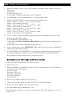
Figure 19.2 Edge surface example 2 – 3D with edit vertices.
modelling with AutoCAD.qxd 17/06/2002 15:39 Page 129
13 Use the N/D/L/R/U options and enter the following new locations for the named vertices:
relative movement vertices
@0,0,50 9,0 10,1
@0,0,40 8,0 9,1 10,2
@0,0,30 7,0 8,1 9,2 10,3
@0,0,20 6,0 7,1 8,2 9,3 10,4
@0,0,10 5,0 6,1 7,2 8,3 9,4 10,5
14 When all the new vertex locations have been entered:
a) enter X <R> to exit the edit vertex option
b) then enter X <R> to end the command
15 The mesh will be displayed with a ‘raised corner’ as fig(c)
16 At the command line enter PEDIT <R> then:
a) pick any point on the mesh
b) enter E <R> for the edit vertex option
c) use the N/U/R/L/D entries to move the X to the following named vertices and with
the M (move option), enter the following new locations:
relative movement vertices
@0,0,–80 4,10
@0,0,–50 3,10 4,9 5,10
@0,0,–30 2,10 3,9 4,8 5,9 6,10
@0,0,–10 1,10 2,9 3,8 4,7 5,8 6,9 7,10
d) exit the vertex option with X <R>
e) exit the polyline edit command with X <R>
17 These vertex modifications have produced a v-type notch in the mesh as fig(d)
18 Paper space and zoom-previous then model space. Freeze the MODEL layer
19 The complete four viewport configuration of the edge surface mesh is displayed in fig(e)
20 The exercise is now complete – save if required.

21 Now investigate the effect of the smooth surface option (S) on the mesh
Example 3 (an edge surface mesh created from splines)
This example will demonstrate how an edge surface can be stretched between four spline
curves to simulate a car body panel.
1 Open your MV3DSTD template file as usual, i.e. MVLAY1 tab, layer MODEL and UCS BASE
2 Zoom centre about the point (–100,50,50) at 225 magnification in the 3D viewport and
200 in the other three
3 With the lower left viewport active, refer to Fig. 19.3 and by selecting the SPLINE icon
from the Draw toolbar, draw four spline curves using the following coordinate
information. Use the start and end coordinates as the start and end tangents, indicated
by (S) and (E) in the following data table:
spline 1 spline 2 spline 3 spline 4
0,0,0 (S) –200,0,0 (S) –200,80,105 (S) 0,0,0 (S)
–200,0,0 (E) –200,0,100 0,100,105 (E) 0,0,110
<RETURN> –200,80,105 (E) <RETURN> 0,100,105 (E)
<RETURN> <RETURN>
4 The four spline curves will be displayed as fig(a)
5 Make a new layer, MESH colour blue and current
130 Modelling with AutoCAD 2002
modelling with AutoCAD.qxd 17/06/2002 15:39 Page 130
6 Set both SURFTAB1 and SURFTAB2 to 18
7 Using the Edge Surface icon, pick the four spline curves
8 Task
a) Use the View-Hide sequence in the four viewports, and you will probably not notice
any difference
b) Gouraud shade the four viewports and the effect is impressive
c) Use the 3D orbit command in the 3D viewport, and real-time rotate the shaded model.
This is really impressive.
9 Save if required, as this completes the edge surface exercises.
Summary

1 An edge surface is a polygon mesh stretched between four touching objects – lines, arcs,
splines or polylines
2 An edge surface mesh can be edited with the polyline edit command
3 The added surface is a COONS patch and is bicubic, i.e. one curve is defined in the mesh
M direction and the other is defined in the mesh N direction
4 The first curve (edge) selected determines the mesh M direction and the adjoining curves
define the mesh N direction
5 The mesh density is controlled by the system variables:
a) SURFTAB1: in the mesh M direction
b) SURFTAB2: in the mesh N direction
Edge surface 131
Figure 19.3 Edge surface example 3 – using splines.
modelling with AutoCAD.qxd 17/06/2002 15:39 Page 131
6 The default value for SURFTAB1 and SURFTAB2 is 6
7 The type of mesh stretched between the four curves is controlled by the SURFTYPE
system variable and:
a) SURFTYPE 5 – Quadratic B-spline
b) SURFTYPE 6 – Cubic B-spline (default)
c) SURFTYPE 8 – Bezier curve
8 The SURFTYPE variable controls the appearance of all mesh curves.
Assignment
MACFARAMUS was contracted by the emperor TOOTENCADUM to create a flat topped
hill for a future project.
The activity is very similar to the second example, i.e. an edge surface has to have several
of its vertices modified to give a ‘flat-top hill’ effect. The process is quite tedious, but
persevere with it as it is needed for another activity in a later chapter.
Activity 13: The flat topped hill made by MACFARAMUS.
1 Use your MV3DSTD template file with UCS BASE as usual
2 Zoom centre about 0,0,50 at 400 magnification originally
3 With layer MODEL, create four touching polyline arcs of radius 200 with 0,0 as the arc

centre point. If you are unsure of this, use the Centre, Start, End ARC option.
4 Make a new layer called HILL, colour green and current
5 Set SURFTAB1 and SURFTAB2 to 20
6 Add an edge surface to the four touching arcs
7 In paper space, zoom the 3D viewport then return to model space
8 Use the Modify-Object-Polyline (PEDIT) command with the Edit Vertex option to move
the following vertices by @0,0,100:
a) 6,9 6,10 6,11
b) 7,7 7,8 7,9 7,10 7,11 7,12 7,13
c) 8,7 8,8 8,9 8,10 8,11 8,12 8,13
d) 9,6 9,7 9,8 9,9 9,10 9,11 9,12 9,13 9,14
e) 10,6 10,7 10,8 10,9 10,10 10,11 10,12 10,13 10,14
f) 11,6 11,7 11,8 11,9 11,10 11,11 11,12 11,13 11,14
g) 12,7 12,8 12,9 12,10 12,11 12,12 12,13
h) 13,7 13,8 13,9 13,10 13,11 13,12 13,13
i) 14,9 14,10 14,11
9 Note
a) The named vertices all lie within a circle of radius 100
b) Use the N/U/D/L/R entries of the edit vertex option until the named vertex is displayed
then use the M option with an entry of @0,0,100
10 When all the vertices have been modified, optimise your viewpoints. I used four different
VPOINT-ROTATE values and the effect with hide was quite ‘pleasing’
11 Save this drawing as MODR2002\HILL as it will be used with a later activity.
12 The View-Shade-Gouraud Shaded effect in any 3D viewport with the 3D orbit command
is very interesting. You can rotate the model to ‘see inside’ the raised part of the edge
surface.
132 Modelling with AutoCAD 2002
modelling with AutoCAD.qxd 17/06/2002 15:39 Page 132
3D polyline
A 3D polyline is a continuous object created in 3D space. It is similar to a 2D polyline,

but does not possess the 2D versatility, i.e. there are no variable width or arc options
available with a 3D polyline. The benefit of a 3D polyline is that it allows x,y,z coordinates
to be used. A 2D polyline can only be created in the plane of the current UCS.
Example
This exercise will create a series of hill contours from splined 3D polylines, so:
1 Open your MV3DSTD template file, MVLAY1 tab with the lower left viewport active and
UCS BASE.
2 Refer to Fig. 20.1 and make the following new layers:
LEVEL1, LEVEL2, LEVEL3, LEVEL4 – all colour green
PATH1: red; PATH2: blue; PATH3: magenta
3 With layer LEVEL1 current, menu bar with Draw-3Dpolyline and:
prompt Specify start point of polyline and enter: 0,50,0 <R>
prompt Specify endpoint of line and enter: 50,0,0 <R>
prompt Specify endpoint of line and enter: 150,0,0 <R>
prompt Specify endpoint of line and enter: 220,60,0 <R>
prompt Specify endpoint of line and enter: 260,140,0 <R>
prompt Specify endpoint of line and enter: 170,180,0 <R>
prompt Specify endpoint of line and enter: 20,160,0 <R>
prompt Specify endpoint of line and enter: c <R>
4 Make layer LEVEL2 current and at the command line enter 3DPOLY <R> and:
prompt Specify start point of polyline and enter: 40,60,50 <R>
prompt Specify endpoint of line and enter: 80,20,50 <R>
prompt Specify endpoint of line and enter: 140,35,50 <R>
prompt Specify endpoint of line and enter: 200,100,50 <R>
prompt Specify endpoint of line and enter: 130,140,50 <R>
prompt Specify endpoint of line and enter: 60,130,50 <R>
prompt Specify endpoint of line and enter: c <R>
5 With layers LEVEL3 and LEVEL4 current, use the 3D polyline command with the
following coordinate values:
Level3 Level4

Start point 70,70,100 85,70,125
Endpoint 80,35,100 90,50,125
Endpoint 130,45,100 130,60,125
Endpoint 170,90,100 130,80,125
Endpoint 100,120,100 close
Endpoint close
Chapter 20
modelling with AutoCAD.qxd 17/06/2002 15:39 Page 133
6 Menu bar with Modify-Object-Polyline and:
prompt Select polyline
respond pick the 3D polyline created at level 1
prompt Enter an option
enter S <R> – the spline option
prompt Enter an option
enter X <R> – the exit command option
7 The selected polyline will be displayed as a splined curve
8 Use the S option of the Edit Polyline command to spline the other three 3D polylines
9 Zoom centre about 120,90,60 at 200 magnification in all viewports
10 With layer PATH1 current, use the 3D polyline command with the following entries:
Start: 0,50,0 – level 1 point
Endpoint: 60,130,50 – level 2 point
Endpoint: 100,120,100 – level 3 point
Endpoint: 130,60,125 – level 4 point
Endpoint: <R>
11 This 3D polyline is a path ‘up the hill’ and each entered coordinate value is a point on
the level 1,2,3,4 contours
12 Spline this polyline, and it does not pass through the entered coordinates
134 Modelling with AutoCAD 2002
Figure 20.1 3D polyline example.
modelling with AutoCAD.qxd 17/06/2002 15:39 Page 134

13 Task
a) Using the ID command, identify the coordinates of the points A, B and C where PATH1
‘crosses’ the level 2, 3 and 4 contours. My values were:
ptA: 55.06, 101.57, 50
ptB: 95.42, 101.91, 100
ptC: 127.07, 65.65, 125
b) With layer PATH2 current, create a 3D polyline as a ‘path down the hill’, this path to
be drawn as a vertical line in the top (lower right) viewport. It has to ‘touch’ each
contour, and if possible, be the shortest distance (ortho on helps, as does OSNAP
nearest). Do not spline this path. Find the distance from top to bottom for this path.
My value was 135.51.
c) With layer PATH3 current, create another un-splined 3D polyline which is to ‘join the
four level right-ends’ in the top right viewport. Find the distance between each level
for this path.
My three values were:
1–2: 82.81
2–3: 57.69
3–4: 38.26
14 The exercise is now complete. Save if required.
Summary
1 A 3D polyline is a single object and can be used with x,y,z coordinate entry
2 A 3D polyline can be edited with options of Edit vertex, Spline and decurve
3 3D polylines cannot be displayed with varying width or with arc segments.
4 The command is activated from the menu bar or by command line entry.
3D polyline 135
modelling with AutoCAD.qxd 17/06/2002 15:39 Page 135
3D objects
AutoCAD has nine pre-defined 3D objects, these being box, pyramid, wedge, dome,
sphere, cone (and cylinder), torus, dish and mesh. They are considered as ‘meshes’ and
can be displayed with hide, shade and render.

To demonstrate some of these objects:
1 Open your MV3DSTD template file, with MVLAY1 tab, layer MODEL, UCS BASE and
the lower left viewport active.
2 Refer to Fig. 21.1 and display the Surfaces toolbar
3 In the steps which follow, reason out the coordinate entry values
4 Select the BOX icon from the Surfaces toolbar and:
prompt Specify corner point of box and enter: 0,0,0 <R>
prompt Specify length of box and enter: 150 <R>
prompt Specify width of box and enter: 120 <R>
prompt Specify height of box and enter: 100 <R>
prompt Specify rotation angle of box about Z axis and enter: 0 <R>
5 A red box will be displayed at the 0,0,0 origin point
6 Menu bar with Draw-Surfaces-3D Surfaces and:
prompt 3D Objects dialogue box
respond pick Wedge then OK
prompt Specify corner point of wedge and enter: 150,0,0 <R>
prompt Specify length of wedge and enter: 80 <R>
prompt Specify width of wedge and enter: 70 <R>
prompt Specify height of wedge and enter: 150 <R>
prompt Specify rotation angle of wedge about Z axis and enter: –10 <R>
7 At the command line enter CHANGE <R> and:
prompt Select objects and pick the wedge then right-click
prompt Specify change point or [Properties] and enter: P <R>
prompt Enter property to change and enter: C <R> – colour option
prompt Enter new colour and enter: 14 <R>
prompt Enter property to change and <RETURN>
8 Using the icons from the Surfaces toolbar, or the 3D Objects dialogue box, create the
following two 3D objects:
Cone Cylinder (using cone object)
Base centre: 50,70,100 Base centre: 75,0,50

Radius for base: 50 Radius for base: 50
Radius for top: 0 Radius for top: 50
Height: 85 Height: 90
Number of segments: 16 Number of segments: 16
Colour: green Colour: blue
9 Restore UCS RIGHT and with the ROTATE icon from the Modify toolbar:
a) pick the blue cylinder then right-click
b) base point: 0,50
c) rotation angle: 90
Chapter 21
modelling with AutoCAD.qxd 17/06/2002 15:39 Page 136
10 Restore UCS BASE
11 Create the following two 3D objects:
Dish Torus
Centre of dish: 75,60,0 Centre of torus: 75,–90,50
Radius: 60 Radius of torus: 100
Longitudinal segments: 16 Radius of tube: 20
Latitudinal segments: 16 Tube segments: 16
Colour: magenta Torus segments: 16
Colour: cyan
12 With the ROTATE icon:
a) pick the cyan torus then right-click
b) base point: –90,50
c) angle: 90
13 Restore UCS BASE
14 Zoom centre about 75,0,50 at 300 magnification
15 Hide and shade to display the model with ‘bright’ colours
16 Task
Still with the MVLAY1 tab active:
a) enter paper space and make layer VP current

b) menu bar with View-Viewports-1 Viewport and make a new viewport selecting one
of the points ‘outwith’ the original four as shown in Fig. 21.1
c) display the model in this new viewport from below and zoom centre about the same
point as before
d) Question: why did we pick one of the new viewport points outwith the original
viewports?
e) Gouraud shade the model in each viewport, then convert back to 2D wireframe.
17 Save the layout, although we will not use it again
3D objects 137
Figure 21.1 3D objects example.
modelling with AutoCAD.qxd 17/06/2002 15:39 Page 137