Modelling with AutoCAD 2002 Episode 7 doc

Shading and 3D orbit
Shading and 3D orbit have been used in previous chapters without any discussion. In
this chapter we will investigate both topics in greater detail.
Shading
Shading allows certain models to be displayed on the screen as a more realistic coloured
image. The models which can be shaded (and rendered) are 2
1
/2D extruded models, 3D
objects, 3D surface models and solid models. We will use some previously created 3D
surface models to investigate the topic.
1 Open the ruled surface model MODR2002\ARCHES from chapter 14
2 Make the model tab active and restore UCS BASE. Any layer can be active
3 a) Menu bar with View-Hide to display the model with hidden line removal. Note the
2D icon is still displayed
b) Menu bar with View-Regen to restore original model
4 a) Menu bar with View-Shade-Hidden and the model will be displayed with hidden
line removal, but note the coloured 3D icon with X-axis red, Y-axis green and Z-axis
blue
b) Menu bar with View-Regen and model is unchanged
c) Menu bar with View-Shade-3D Wireframe and the model will be displayed without
hidden line removal, but the coloured 3D icon is still displayed
d) Menu bar with View-Shade-2D Wireframe to restore the original model with the
2D icon
5 Using the menu bar sequence View-Shade, activate the four shade options returning
the display to 3D Wireframe before activating the next option. Note the difference in
the shading between the Flat and Gouraud options, evident at the arch curved ‘shoulders.
Explanation of the shade options
Activating SHADE from the View pull-down menu allows the user access to seven
options. These options allow models to be displayed as shaded/wireframe images as
follows:
1 2D Wireframe:

The model is displayed with the boundaries as lines and curves with the ‘normal’ 2D
icon. This option is generally used to restore shaded models to their original appearance.
2 3D Wireframe:
Models are displayed as lines and curves for their boundaries but with a coloured 3D
icon. When used, this option restores shaded models to their original appearance but
retains the coloured 3D icon.
Chapter 26
modelling with AutoCAD.qxd 17/06/2002 15:40 Page 173
3 Hidden:
Displays models with hidden line removal and displays the coloured 3D icon. The REGEN
command will not work when this option has been used, and models are restored to
their original appearance with either the 2D Wireframe or 3D Wireframe options.
4 Flat Shaded:
Models are shaded between their polygon mesh faces and appear flatter and less smooth
than the Gouraud shaded models. Any materials (later chapter) which have been applied
are also displayed flat shaded
5 Gouraud Shaded:
Models are shaded with the edges between the polygon mesh faces smoothed. This
option gives models a realistic appearance. Added materials are also Gouraud shaded.
6 Flat Shaded, Edges On:
Models are flat shaded with the wireframe showing through the shade effect
7 Gouraud Shaded, Edges On:
Models displayed with the Gouraud shading effect and the wireframe shows through
8 General:
a) Both the Flat and Gouraud shading options display the coloured 3D icon
b) The Flat and Gouraud shading use the 2D wireframe or the 3D Wireframe options to
restore the model to its original appearance
c) The REDRAW/REGEN/REGENALL commands cannot be used if the View-Shade
sequence is activated
d) If HIDE <R> is entered from the command line to display any model with hidden

line removal, then REGEN can be used.
This completes the shading part of the chapter. Ensure that the ARCHES drawing is still
displayed in the model tab for the 3D orbit exercise.
3D orbit
The 3D orbit command (introduced in AutoCAD Release 2000) allows real-time 3D
rotation, the user controlling this rotation with the pointing device. The basic concept
is that you are viewing the model (the target) with a camera (the user), the target
remaining stationary while the camera moves around the target. The opposite effect is
displayed on the screen, i.e. the models appears to ‘rotate’.
The 3D orbit concept has its own terminology, the most common being the arcball and
icons – Fig. 26.1.
1 Arcball: is a circle with smaller circles at the quadrants
2 Icons: which alter in appearance dependent on were the pointing device is positioned
relative to the arcball
3 Click and drag: the term for holding down the left button of the mouse and moving the
mouse to give rotation of the model
4 Roll: a type of rotation when the icon is outside the arcball. It is a rotation about an axis
through the centre of the arcball perpendicular to the screen.
174 Modelling with AutoCAD 2002
modelling with AutoCAD.qxd 17/06/2002 15:40 Page 174
Using 3D orbit
1 The ARCHES model should still be displayed in Model tab
2 Pick the 3D Orbit icon from the Standard toolbar and:
prompt Arcball displayed
respond a) hold down the left mouse button
b) move the mouse about the screen
c) release the mouse button
d) practice this hold down, move, release and note the movement of the model
e) press ESC to end command
3 Restore the model to its original viewpoint with U <R>

4 Menu bar with View-Shade-Gouraud Shaded
5 At the command line enter 3DORBIT <R> and:
prompt Arcball displayed
respond right-click
prompt Shortcut menu
respond pick More
prompt cascade shortcut menu – Fig. 26.2
respond pick Continuous Orbit
prompt continuous icon displayed
respond 1. move mouse slightly then leave it alone
2. model displayed shaded with continuous rotation
3. use the mouse left button to alter the rotation
4. practice the continuous rotation
5. right-click and pick Exit
6 Restore the model to the original orientation with U <R>
Shading and 3D orbit 175
Figure 26.1 The basic 3D orbit terminology.
modelling with AutoCAD.qxd 17/06/2002 15:40 Page 175
The 3D orbit shortcut menu
When the 3D orbit command is active, a right-click will display the shortcut menu which
has been used to select the More and Exit options. The shortcut menu allows the user
access to several useful and powerful options, the complete list being:
a) Exit: does what it says, it exits the command
b) Pan: the real-time AutoCAD pan command
c) Zoom: the real-time AutoCAD zoom command, i.e. movement upwards
gives magnification of model, movement downwards gives a
reduction
d) Orbit: indicates that the command is active/inactive
e) More: allows the user access to an additional ten options which include
Adjust Distance, Swivel Camera, Continuous Orbit, Clipping

Planes
f) Projection: allows parallel or perspective selections
g) Shading Modes: allows selection of the normal AutoCAD shading
h) Visual Aids: compass, grid and UCS icon
i) Reset View: a useful selection as it restores the model to its original orientation
prior to using the orbit command and should be used instead of the
U <R> used previously
j) Preset Views: allows the normal 3D views to be activated
Using the shortcut menu is straightforward so:
1 Activate the 3D orbit command and start rotating the model
2 Press the right button
3 Select the required option, e.g. Shading Modes-Flat Shaded
4 Display restored and the 3D rotation can continue
The visual aids selection allows the user to display:
a) a compass: a sphere is displayed inside the arcball consisting of three circles
representing the X, Y and Z axes. This sphere rotates with the model
b) A grid: draws an array of lines on a plane parallel to the current X and Y axes,
perpendicular to the Z axis.
176 Modelling with AutoCAD 2002
Figure 26.2 The 3D Orbit shortcut menu.
modelling with AutoCAD.qxd 17/06/2002 15:40 Page 176
The clipping planes
The clipping plane options in 3D orbit are similar to the clip option of the DVIEW
command, i.e. the clipping plane is an invisible plane set by the user. Parts of the model
can be clipped, i.e. ‘cut-away’ relative to this clipping plane. To demonstrate the option:
1 Restore the model to its original orientation
2 Start the model rotating with the 3D orbit command
3 Activate the shortcut menu and select the Hidden shading mode
4 Activate the shortcut menu and select More-Adjust Clipping Plane and:
prompt Adjust Clipping Plane dialogue box

respond 1. pick the Adjust Front Clipping icon
2. drag the datum plane downwards – Fig. 26.3(a)
3. right-click and close
5 Continue with the 3D orbit and the model will be rotated with a front clip effect –
Fig. 26.3(b)
6 When you are satisfied with the display:
a) right-click and reset view
b) right-click and exit
7 The model should be restored to its original orientation
8 Try this clipping plane option a few times. It is relatively easy to use.
Shading and 3D orbit 177
Figure 26.3 Using the More-Adjust Clipping Planes option of 3D orbit.
Adjust Front Clipping
(a) (b)
modelling with AutoCAD.qxd 17/06/2002 15:40 Page 177
The 3D Orbit toolbar
The toolbar for the 3D orbit command is displayed in Fig. 26.4 and allows the user access
to:
a) 3D pan and 3D zoom
b) the 3D orbit, swivel and continuous rotations
c) the 3D adjust distance
d) the clipping plane options: adjust, front and back
e) selecting the current 3D view
This completes the chapter on shading and 3D orbit.
Summary
1 Surface and solid models can be shaded, the two options being Flat and Gouraud
2 Gouraud shaded models appear smoother than flat shaded models and this is the
suggested mode for all future shading
3 The 3D orbit command allows interactive real-time 3D rotation of models – shaded or
unshaded, with/without hidden line removal

4 The user has access to several useful options when the 3D orbit command is being used.
These include parallel and perspective views of the model, front and back clipping and
continuous 3D orbit
5 The user should become familiar with using the 3D orbit command as it will be used
with solid modelling.
178 Modelling with AutoCAD 2002
Figure 26.4 The 3D Orbit toolbar.
Pan
Zoom
3D Orbit
Continuous Orbit
3D Swivel
3D Views selection
Back Clip On/Off
Front Clip On/Off
3D Adjust Clip Planes
3D Adjust Distance
modelling with AutoCAD.qxd 17/06/2002 15:40 Page 178
Introduction to solid
modelling
Three dimensional modelling with computer-aided draughting and design (CADD) can
be considered as three categories:
• wire-frame modelling
• surface modelling
• solid modelling
We have already created wire-frame and surface models and will now concentrated on
how solid models are created.
This chapter will summarise the three model types.
Wire-frame modelling
1 Wire-frame models are defined by points and lines and are the simplest possible

representation of a 3D component. They may be adequate for certain 3D model
representation and require less memory than the other two 3D model types, but wire-
frame models have several limitations:
a) Ambiguity: it is difficult to know how a wire-frame model is being viewed, i.e. from
above or from below?
b) No curved surfaces: while curves can be added to a wire-frame model as arcs or trimmed
circles, an actual curved surface cannot. Lines may be added to give a ‘curved effect’
but the computer does not recognise these as being part of the model.
c) No interference: as wire-frame models have no surfaces, they cannot detect interference
between adjacent components. This makes then unsuitable for kinematic displays,
simulations etc.
d) No physical properties: mass, volume, centre of gravity, moments of inertia, etc. cannot
be calculated
e) No shading: as there are no surfaces, a wire-frame model cannot be shaded or rendered.
f) No hidden line removal: as there are no surfaces, it is not possible to display the model
with hidden line removal.
2 AutoCAD 2002 allows wire-frame models to be created.
Chapter 27
modelling with AutoCAD.qxd 17/06/2002 15:40 Page 179
Surface modelling
1 A surface model is defined by points, lines and faces. A wire-frame model can be
‘converted’ into a surface model by adding these ‘faces’. Surface models have several
advantages when compared to wire-frame models, some of these being:
a) Recognition and display of curved profiles
b) Shading, rendering and hidden line removal are all possible, i.e. no ambiguity
c) Recognition of holes
2 Surface models are suited to many applications but they have some limitations which
include:
a) No physical properties: other than surface area, a surface model does not allow the
calculation of mass, volume, centre of gravity, moments of inertia, etc.

b) No detail: a surface model does not allow section detail to be obtained.
3 Several types of surface model can be generated including:
a) plane and curved swept surfaces
b) swept area surfaces
c) rotated or revolved surfaces
d) splined curve surfaces
e) nets or meshes
4 AutoCAD 2002 allows surface models of these types to be created.
Solid modelling
1 A solid model is defined by the volume the component occupies and is thus a real 3D
representation of the component. Solid modelling has many advantages which include:
a) Complete physical properties of mass, volume, centre of gravity, moments of inertia, etc.
b) Dynamic properties of momentum, angular momentum, radius of gyration, etc.
c) Material properties of stress-strain
d) Full shading, rendering and hidden detail removal
e) Section views and profile extraction
f) Interference between adjacent components can be highlighted
g) Simulation for kinematics, robotics, etc.
2 Solid models are created using a solid modeller and there are several types of solid
modeller, the two most common being:
a) Constructive solid geometry or constructive representation, i.e. CSG/CREP. The model
is created from solid primitives and/or swept surfaces using Boolean operations
b) Boundary representation (BREP). The model is represented by the edges and faces
making up the surface, i.e. the topology of the component.
3 AutoCAD 2002 supports solid models of the CSG/CREP type.
4 The AutoCAD 2002 modeller is based on the ACIS solid modeller and supports NURBS
– nonuniform rational B splined curves
180 Modelling with AutoCAD 2002
modelling with AutoCAD.qxd 17/06/2002 15:40 Page 180
Comparison of the model types

The three model types are displayed in:
a) Figure 27.1: as models with hidden line removal
b) Figure 27.2: as model cross-sections
Introduction to solid modelling 181
Figure 27.1 Simple comparison between wire-frame, surface and solid models.
Figure 27.2 Further comparison of model types as cross-sections.
modelling with AutoCAD.qxd 17/06/2002 15:40 Page 181
The solid model standard sheet
A solid model standard sheet (prototype drawing) will be created as a template and
drawing file using the layouts from the surface model exercises, i.e. MV3DSTD. This
standard sheet will:
a) be for A3 paper
b) have the four tab configurations: Model, Layout1, Layout2 and Layout3
1 Close and existing drawings or start AutoCAD
2 Menu bar with File-New and open your MV3DSTD template or drawing file
3 Check the following:
a) Tool-Named UCS: BASE, FRONT, RIGHT – set and saved
b) Layers: 0,DIM,MODEL,OBJECTS,SECT,SHEET,TEXT,VP
c) Sheet: layout to your own specification
d) Text style: ST1 (romans.shx) and ST2 (Arial Black)
e) Dimension style: 3DSTD with various settings
4 At the command line enter -PURGE <R> and:
prompt Enter type of unused objects to purge
enter LA <R> – layer option
prompt Enter names to purge<*> and <RETURN>
prompt Verify each name to be purges [Yes/No] and enter: Y <R>
prompt Purge layer “DIM” and enter: N <R>
prompt Purge layer “OBJECTS” and enter: Y <R>
prompt Purge layer “SECT” and enter: N <R>
prompt Purge layer “TEXT” and enter: N <R>

5 Repeat the command line -PURGE command with the following entries:
a) B (blocks) and purge all (if any) blocks
b) D (dimstyles) and purge all dimension styles except 3DSTD
c) ST (text styles) and purge any text styles except ST1 and ST2
d) SH (shapes) and purge all (if any) shapes
e) M (multilines) and purge all (if any) multilines
f) Note: entering PURGE at the command line will allow the user access to the Purge
dialogue box. The various unwanted items can then be purged from the standard sheet
6 At the command line enter ISOLINES <R> and:
prompt Enter new value for ISOLINES<4>
enter 12 <R>
6 At the command line enter FACETRES <R> and:
prompt Enter new value for FACETRES<0.5000>
enter 1 <R>
7 Display the Draw, Modify, Object Snap and Solids toolbars
8 Make MVLAY1 tab current, model space with the lower left viewport active, restore UCS
BASE with layer MODEL current
182 Modelling with AutoCAD 2002
modelling with AutoCAD.qxd 17/06/2002 15:40 Page 182
9 Menu bar with File-Save As and:
prompt Save Drawing As dialogue box
respond 1. scroll at Files of type
2. pick AutoCAD Drawing Template File (*.dwt)
prompt Save in AutoCAD Template folder dialogue box
respond 1. enter file name as: A3SOL.dwt
2. pick Save
prompt Template Description dialogue box
respond 1. enter: My solid model prototype created on ???
2. measurement: Metric
then pick OK

10 Menu bar with File-Save As and:
prompt Save Drawing As dialogue box
respond 1. scroll at Files of type
2. pick AutoCAD 2000 Drawing (*.dwg)
3. scroll and pick your named folder
4. enter file name: A3SOL.dwg
5. pick Save
11 Menu bar with File-Save As and save you standard sheet as an AutoCAD Drawing
Template file (A3SOL) in your named folder
12 You are now ready to start creating solid models.
Notes
1 The new A3SOL solid model standard sheet has been saved as both a template file and
a drawing file
2 The A3SOL drawing file has been saved to your named folder, while the template file
has been saved to both the AutoCAD Template folder and your named folder.
3 Two new system variables have been introduced in the creation of the A3SOL
template/drawing file, these being:
ISOLINES: specifies the number of isolines per surface on objects. It is an integer with
values between 0 and 2047. The default value is 4.
FACETRES: adjusts the smoothness of shaded and rendered objects and objects with
hidden line. The value can be between 0.01 and 10.00, the default being 0.5
4 The ISOLINES and FACETRES values may be altered when creating some models
5 The viewports have not been zoom-centred, as this will depend on the model being
created.
6 Solid modelling consists of creating ‘composites’ from ‘primitives’ and AutoCAD 2002
supports the following types of primitive:
a) basic b) swept c) edge
7 All three types of primitive will be investigated with examples and the various options
for each will be discussed.
8 While the A3SOL standard sheet has different layout configurations, I will generally only

use the MVLAY1 or the MODEL tabs the, although the other layout tabs will be
‘investigated’ from time to time
Solid modelling is a fascinating topic, and should give the user a great deal of satisfaction
as the various models are created and rendered.
Introduction to solid modelling 183
modelling with AutoCAD.qxd 17/06/2002 15:40 Page 183
The basic solid
primitives
AutoCAD 2002 supports the six basic solid primitives of box, wedge, cylinder, cone,
sphere and torus. In this chapter we will create layouts (which I hope are interesting)
using each primitive. We will also investigate the various options which are available.
Note: During the exercises do not just accept the coordinate values given. Try and reason
out why they are being used.
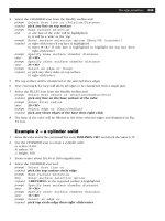
The BOX primitive – Fig. 28.1
1 Open your A3SOL template file with layer MODEL, tab MVLAY1, UCS BASE and the
lower left viewport active. Display the Object Snap and Solids toolbars.
2 Select the BOX icon from the Solids toolbar and:
prompt Specify corner of box or [CEnter]<0,0,0>
enter 0,0,0 <R>
prompt Specify corner or [Cube/Length]
enter C <R> – the cube option
prompt Specify length
enter 100 <R>
and a red cube is displayed in all viewports
3 Select from the menu bar Draw-Solids-Box and:
prompt Specify corner of box or [CEnter]<0,0,0>
enter 100,0,0 <R>
prompt Specify corner or [Cube/Length]
enter L <R> – the length option
prompt Specify length and enter: 40 <R>

prompt Specify width and enter: 80 <R>
prompt Specify height and enter: 30 <R>
and another red cuboid is displayed in all viewports
4 At the command line enter CHANGE <R> and:
prompt Select objects
respond pick the smaller box then right-click
prompt Specify change point or [Properties] and enter: P <R>
prompt Enter property to change and enter: C <R>
prompt Enter new color and enter: 3 <R> or green <R>
prompt Enter property to change and right-click/enter
5 Now zoom-extents the zoom at a scale of 1.5 in each viewport then make the lower left
viewport again active
Chapter 28
modelling with AutoCAD.qxd 17/06/2002 15:40 Page 184
6 At the command line enter BOX <R> and:
prompt Specify corner of box or [CEnter]<0,0,0>
respond Endpoint icon and pick pt1 – first corner point
prompt Specify corner or [Cube/Length]
enter @120,60,15 <R> – the diagonally opposite corner point
7 Change the colour of this box to blue, with CHANGE <R> at the command line as
step 4
8 Restore UCS RIGHT
9 Create a solid box with the following information:
a) corner: 0,70,100
b) cube option with length: 25
10 a) At the command line enter CHANGE <R> and:
prompt Select objects
respond pick the last box created
prompt 1 was not parallel to the UCS
respond right-click to end the command

b) At the command line enter CHPROP <R> and:
prompt Select objects
respond pick the last box created and right-click
prompt Enter property to change and enter: C <R>
prompt Enter new color and enter: MAGENTA <R>
prompt Enter property to change and right-click/enter
c) Note: the CHANGE and CHPROP commands will be discussed at the end of the
chapter. In future, when an object has to have its colour changed use the CHPROP
command from the command line.
The basic solid primitives 185
Figure 28.1 The BOX primitive layout (BOXPRIM).
modelling with AutoCAD.qxd 17/06/2002 15:40 Page 185
11 Rectangular array the magenta box:
a) for 1 row and 3 columns
b) with column distance: 30
12 Restore UCS FRONT
13 Activate the solid BOX command and:
prompt Specify corner of box or [CEntre]<0,0,0>
enter CE <R> – the box center point option
prompt Specify center of box and enter: 50,80,30 <R>
prompt Specify corner of box or [Cube/Length] and enter: L <R>
prompt Specify length and enter: 18 <R>
prompt Specify width and enter: 25 <R>
prompt Specify height and enter: 60 <R>
14 With CHPROP, change the colour of this last box to suit yourself. I used colour number 76
15 Polar array this last box with:
a) center point: 50,50
b) items: 4
c) 360 angle with rotation
16 Finally restore UCS BASE and create another solid box with:

a) corner: 0,100,100
b) length: –10; width: –80; height: –65
c) colour: number 234
17 The model is now complete so save as MODR2002\BOXPRIM
18 Investigate:
a) The model with hide – menu bar or command line
b) Shading the viewports
c) The 3D orbit command with the shaded model and the model tab active
d) Restoring the model to the original 3D wireframe display
19 Changing properties
When solid model layouts are being created the user will be asked to change some
properties, especially the colour. All primitives will be originally displayed as red (due
to layer MODEL being current) and thus require to be changed to another colour. This
is to give a coloured image for shading, rendering and for using the 3D orbit command
to maximum effect. Changing the colour of a primitive depends on the value of the
PICKFIRST system variable and:
a) if PICKFIRST is set to 0, then use CHANGE <R> at the command line as step 4, i.e.
activate the command then pick the object which is to have its colour changed
b) If PICKFIRST is set to 1 then:
1. select the object to be changed
2. pick the Properties icon from the Standard toolbar
3. pick the Color line
4. scroll and pick the required colour
5. cancel the Properties dialogue box and press ESC
20 CHANGE or CHPROP?
These two commands are similar but:
a) CHANGE can only be used for objects created with the current UCS, hence the step
10(a) message
b) CHPROP can be used with ANY UCS setting, and should be used for all future change
colour operations

21 The user must now decide whether to set PICKFIRST to 0 or 1. My personal preference
is to have PICKFIRST set to 0 and use the CHPROP command.
186 Modelling with AutoCAD 2002
modelling with AutoCAD.qxd 17/06/2002 15:40 Page 186
The WEDGE primitive – Fig. 28.2
1 Open the A3SOL template file with layer MODEL, MVLAY tab, UCS BASE and lower
left viewport active
2 Menu bar with Draw-Solids-Wedge and:
prompt Specify corner of wedge or [CEnter]<0,0,0>
enter 0,0,0 <R>
prompt Specify corner or [Cube/Length]
enter C <R> – the cube option
prompt Specify length
enter 100 <R>
and red wedge displayed in all viewports
3 Select the WEDGE icon from the Solids toolbar and:
prompt Specify corner of wedge or [CEnter]
enter 0,0,0 <R>
prompt Specify corner or [Cube/Length]
enter @80,–60 <R> – the other corner option
prompt Specify height and enter: 50 <R>
4 Change the colour of this wedge to blue
5 In each viewport, zoom-extents then zoom to a 1.75 scale then make the lower left
viewport again active
The basic solid primitives 187
Figure 28.2 The WEDGE primitive layout (WEDPRIM).
modelling with AutoCAD.qxd 17/06/2002 15:40 Page 187
6 At the command line enter WEDGE <R> and create a solid wedge with:
a) corner: 100,100,0
b) length: 60; width: 60; height: 80

c) colour: green
d) 2D rotate the green wedge about the point 100,100 by –90degs
7 Restore UCS FRONT and create a wedge with:
a) corner: endpoint icon and pick pt1
b) length: –50
c) width: –100
d) height: 30
e) colour: magenta (CHPROP command)
8 Restore UCS BASE
9 The final wedge is to be created with:
a) corner: endpoint of pt2
b) cube option with length: –80
c) colour: number 14
10 Save the model layout as MODR2002\WEDPRIM
11 Hide and shade the model in each viewport
12 Use 3D orbit with a shaded model in the MODEL tab.
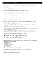
The CYLINDER primitive – Fig. 28.3
1 Open A3SOL, UCS BASE, MVLAY1 tab, layer MODEL, lower left viewport active
2 Menu bar with Draw-Solids-Cylinder and:
prompt Specify center point for base of cylinder or [Elliptical]
enter 0,0,0 <R> – the cylinder base centre point
prompt Specify radius for base of cylinder or [Diameter]
enter 60 <R> – the cylinder radius
prompt Specify height of cylinder or [Center of other end]
enter 100 <R> – the cylinder height
and a red cylinder is displayed, centred on 0,0,0
3 Select the CYLINDER icon from the Solids toolbar and:
prompt Specify center point for base of cylinder or [Elliptical]
enter E <R> – the elliptical option
prompt Specify axis endpoint of ellipse for base of cylinder or

[Center]
enter C <R> – the centre option
prompt Specify center point of ellipse for base of cylinder
enter 80,0,0 <R>
prompt Specify axis endpoint of ellipse for base of cylinder
enter @20,0,0 <R>
prompt Specify length of other axis for base of cylinder
enter @0,30,0 <R>
prompt Specify height of cylinder or [Center of other end]
enter 50 <R>
4 Change the colour of this cylinder to green, then polar array it:
a) about the point 0,0
b) for 3 items, full angle with rotation
5 Zoom centre about the point 0,0,80 at 300 magnification in all viewports
188 Modelling with AutoCAD 2002
modelling with AutoCAD.qxd 17/06/2002 15:40 Page 188
6 At the command line enter CYLINDER <R> and:
prompt Specify center point for base of cylinder or [Elliptical]
enter 60,0,65 <R> – the cylinder base centre point
prompt Specify radius for base of cylinder and enter: 15 <R>
prompt Specify height of cylinder or [Center of other end]
enter C <R> – centre of other end option
prompt Specify center of other end of cylinder
enter @80,0,0 <R>
7 Change the colour of this cylinder to magenta and polar array it with the same entries
as step 4
8 Create another two cylinders:
centre pt rad ht colour
0,0,100 20 50 number 15
0,0,150 70 20 blue

9 Finally create an elliptical cylinder:
a) centre: 70,0,190
b) axis endpoint: @30,0
c) length of other axis: @0,20
d) centre of other end: @–140,0,0
e) colour to suit
10 Save the model as MODR2002\CYLPRIM
11 Hide the model and note the triangular facets which are not displayed when the cylinder
primitives are created. Shade then return the model to wireframe representation
The basic solid primitives 189
Figure 28.3 The CYLINDER primitive layout (CYLPRIM).
modelling with AutoCAD.qxd 17/06/2002 15:40 Page 189
12 Investigate
a) With the 3D viewport active, enter ISOLINES at the command line and enter a value
of 6. Enter REGEN <R> and note model display
b) change the ISOLINES value to 48 and regen
c) return the ISOLINES value to the original 12
d) enter FACETRES at the command line and alter the value to 2, then enter HIDE <R>.
Note the effect, then regen
e) alter FACETRES to 5, hide, then regen
f) return FACETRES to 1
13 Note
The ISOLINES system variable controls the appearance of primitive curved surfaces when
they are created. The triangulation effect, or FACETS, is controlled by the system variable
FACETRES. The higher the value of FACETRES (max 10) then the ‘better the appearance’
of curved surfaces, but the longer it takes for hide and shade. At our level, the values of
12 for ISOLINES and 1 for FACETRES are sufficient.
The CONE primitive – Fig. 28.4
1 Open the A3SOL template file, MVLAY1, UCS BASE etc
2 Menu bar with Draw-Solids-Cone and:

prompt Specify center point for base of cone or [Elliptical]
enter 0,0,0 <R> – the cone base centre point
prompt Specify radius for base of cone or [Diameter]
enter 50<R>
prompt Specify height of cone or [Apex]
enter 60 <R>
3 Create another cone with:
a) centre: 0,0,0
b) radius: 90
c) height: –80
d) colour: green
4 Centre each viewport about the point 0,0,10 at 200 mag
5 Select the CONE icon from the Solids toolbar and:
prompt Specify center point for base of cone or [Elliptical]
enter E <R> – the elliptical option
prompt Specify axis endpoint of ellipse for base of cone or
[Center]
enter C <R> – the centre point option
prompt Specify center point of ellipse for base of cone
enter 70,0,0 <R>
prompt Specify axis endpoint of ellipse for base of cone and enter:
@20,0,0 <R>
prompt Specify length of other axis for base of cone and enter:
@0,25,0 <R>
prompt Specify height of cone or [Apex] and enter: 35 <R>
6 Change the colour of this cone to blue, then polar array it with:
a) centre point: 0,0
b) items: 5
c) full angle to fill, with rotation
190 Modelling with AutoCAD 2002

modelling with AutoCAD.qxd 17/06/2002 15:40 Page 190
7 At the command line enter CONE <R> and:
prompt Specify center point for base of cone and enter: 90,0,0 <R>
prompt Specify radius for base of cone and enter: 15 <R>
prompt Specify height of cone or [Apex]
enter A <R> – the apex option
prompt Specify apex point
enter @40,0,0 <R>
8 Change the colour of this last cone to colour number 235
9 Use the ROTATE 3D command with the last cone and:
a) enter a Y axis rotation
b) enter 90,0,0 as the point on the Y axis
c) enter 41.63 as the rotation angle – why this figure?
10 Polar array the last cone about the point 0,0 for 7 items, full angle with rotation.
11 Create the final cone with:
a) centre: 0,0,75
b) radius: 15
c) apex option: @0,–100,0
d) colour to suit
12 Hide, shade, 3D orbit then save as MODR2002\CONPRIM.
The basic solid primitives 191
Figure 28.4 The CONE primitive layout (CONPRIM).
modelling with AutoCAD.qxd 17/06/2002 15:40 Page 191
The SPHERE primitive – Fig. 28.5
1 Open the A3SOL template file, UCS BASE etc
2 Menu bar with Draw-Solids-Sphere and:
prompt Specify center of sphere<0,0,0>
enter 0,0,0 <R>
prompt Specify radius of sphere or [Diameter]
enter 60 <R>

3 Centre each viewport about 0,0,20 at 200 magnification
4 Select the SPHERE icon from the Solids toolbar and:
prompt Specify center of sphere<0,0,0>
enter 80,0,0 <R>
prompt Specify radius of sphere or [Diameter]
enter D <R> – the diameter option
prompt Specify diameter and enter: 40 <R>
5 Change the colour of this sphere to green, then polar array it:
a) about the point: 0,0
b) for 5 items
c) full angle with rotation
6 At the command line enter SPHERE <R> and create a sphere with:
a) centre: 0,0,75
b) radius: 15
c) colour: magenta
192 Modelling with AutoCAD 2002
Figure 28.5 The SPHERE primitive layout (SPHPRIM).
modelling with AutoCAD.qxd 17/06/2002 15:40 Page 192
7 Restore UCS FRONT and polar array the magenta sphere about the point 0,0 for 3 items
with full angle rotation
8 Restore UCS BASE and create the final sphere with:
a) centre: 58,0,70
b) radius: 30
c) colour blue
d) polar array about 0,0 for 3 items, full angle rotation
9 Hide, shade, save as MODR2002\SPHPRIM
10 Investigate
a) ISOLINES set to 48 then regen
b) ISOLINES set to 5 then regen
c) Restore original ISOLINES 18

d) FACETRES set to 10 then hide and regen
e) Note the appearance of the sphere primitives with these system variable values.
The TORUS primitive – Fig. 28.6
1 A3SOL template file with UCS BASE, MVLAY1 layout etc
2 Menu bar with Draw-Solids-Torus and:
prompt Specify center of torus<0,0,0>
enter 0,0,0 <R>
prompt Specify radius of torus or [Diameter]
enter 80 <R>
prompt Specify radius of tube or [Diameter]
enter 15 <R>
3 Zoom extents then zoom to a scale of 1 in each viewport
4 Restore UCS FRONT and select the TORUS icon from the Solids toolbar and:
prompt Specify center of torus<0,0,0>
enter 80,0,0 <R>
prompt Specify radius of torus and enter: 50 <R>
prompt Specify radius of tube and enter: 20 <R>
5 Change the colour of this torus to blue
6 Restore UCS BASE and polar array the blue torus about 0,0 for 3 items with full circle
rotation
7 Restore UCS RIGHT, enter TORUS <R> at the command line and create a torus with:
a) centre: 0,0,–95
b) radius of torus: 80
c) radius of tube: 20
d) colour: green
8 Restore UCS BASE and create the final torus with:
a) centre: 80,0,80
b) radius of torus: 50
c) radius of tube: 20
d) colour: to suit

9 Save as MODR2002\TORPRIM
The basic solid primitives 193
modelling with AutoCAD.qxd 17/06/2002 15:40 Page 193
10 a) With the lower left viewport active, HIDE and note the effect then regen
b) Enter DISPSILH <R> at the command line and:
prompt Enter new value for DISPSILH <0>
enter 1 <R>
c) Hide the model, note the effect and compare this to that obtained in step (a)
d) Now restore DISPSILH back to 0
11 Note: DISPSILH is a system variable which controls the display of silhouette curves of
solid objects in wire-frame mode and:
DISPSILH 0 : default value, models displayed ‘as normal’
DISPSILH 1 : models displayed with silhouette effect
12 It is your decision as to whether to have DISPSILH set to 0 or 1. I always have it set
to 0.
194 Modelling with AutoCAD 2002
Figure 28.6 The TORUS primitive layout (TORPRIM).
modelling with AutoCAD.qxd 17/06/2002 15:40 Page 194
Summary
1 The six solid primitives can be activated:
a) from the menu bar with Draw-Solids
b) by icon selection from the Solids toolbar
c) by entering the solid name at the command line
2 The corner/centre start points can be:
a) entered as coordinates from the keyboard
b) referenced to existing objects
c) picking suitable points on the screen
3 The six primitives have various options:
box: a) corner; centre
b) cube; length, width, height; other corner

wedge: a) corner; centre
b) cube; length, width, height; other corner
cylinder: a) circular; elliptical
b) radius; diameter
c) height; centre of other end
cone: a) circular; elliptical
b) radius; diameter
c) height; apex point
sphere: a) centre only
b) diameter; radius
torus: a) centre only
b) radius of torus; diameter
c) radius of tube; diameter
Assignment
A single activity for your imaginative mind.
Activity 18: A solid primitive layout.
Create a layout of your own design with the six basic primitives using the following
information and with your own colours:
Box Wedge Cylinder Cone
length: 100 length: 50 radius: 20 radius: 50
width: 40 width: 60 height: 80 height: 120
height: 30 height: 50
Sphere Torus
radius: 40 torus rad: 50
tube rad: 20
The basic solid primitives 195
modelling with AutoCAD.qxd 17/06/2002 15:40 Page 195
The swept solid
primitives
Solid models can be generated by extruding or revolving ‘shapes’ and in this chapter we

will use several exercises to demonstrate how complex solids can be created from
relatively simple shapes.
Extruded solids
Solid models can be created by extruding CLOSED OBJECTS such as polyline shapes,
polygons, circles, ellipses, splines and regions:
a) to a specified height and taper angle
b) along a path.
Extruded example 1: letters
1 Open your A3SOL template file, layer MODEL, MVLAY1 and display the Solids toolbar
2 Change the viewpoint in lower left viewport with the command line entry VPOINT <R>
and:
prompt Specify a view point or [Rotate]
enter R <R> – the rotate option
then enter angles of 30 and 30
3 Make the upper left viewport active and restore UCS RIGHT
4 Using the reference sizes given in Fig. 29.1:
a) draw the three letters M, T and C as closed shapes using line and arc segments
b) use Modify-Object-Polyline from the menu bar to ‘convert’ the three outlines into
a single polyline with the Join option
c) use your discretion for sizes not given (a snap of 5 helps)
d) use the start points A, B and C given
5 Still with UCS RIGHT, zoom centre about 0,50,0 at 200 in the 3D viewport and 300 in
the other three viewports
6 Menu bar with Draw-Solids-Extrude and:
prompt Select objects
respond pick the letter M then right-click
prompt Specify height of extrusion or [Path]
enter 80 <R>
prompt Specify angle of taper for extrusion
enter 0 <R>

7 The letter M will be extruded for a height of 80 in the positive Z direction.
Chapter 29
modelling with AutoCAD.qxd 17/06/2002 15:40 Page 196
8 Select the EXTRUDE icon from the Solids toolbar and:
prompt Select objects
respond pick the letter T then right-click
prompt Specify height of extrusion or [Path]
enter 50 <R>
prompt Specify angle of taper for extrusion
enter 5 <R>
9 At the command line enter EXTRUDE <R> and:
a) objects: pick the letter C then right-click
b) height: enter –50
c) taper angle: enter –3
10 Hide and shade etc, then save the model with your own name
The swept solid primitives 197
Figure 29.1 Extruded example 1 – letters.
modelling with AutoCAD.qxd 17/06/2002 15:40 Page 197