Mechanics.Of.Materials.Saouma Episode 13 pps

Draft
19.4 Plastic Yield Conditions (Classical Models) 5
12 In terms of the principal stresses, those invariants can be simplified into
I
1
= σ
1
+ σ
2
+ σ
3
(19.24)
I
2
= −(σ
1
σ
2
+ σ
2
σ
3
+ σ
3
σ
1
) (19.25)
I
3
= σ
1

σ
2
σ
3
(19.26)
13 Similarly,
J
1
= s
1
+ s
2
+ s
3
(19.27)
J
2
= −(s
1
s
2
+ s
2
s
3
+ s
3
s
1
) (19.28)

J
3
= s
1
s
2
s
3
(19.29)
19.4.1.2 Physical Interpretations of Stress Invariants
14 If we consider a plane which makes equal angles with respect to each of the principal-stress directions,
π plane, or octahedral plane, the normal to this plane is given by
n =
1
√
3



1
1
1



(19.30)
The vector of traction on this plane is
t
oct
=

1
√
3



σ
1
σ
2
σ
3



(19.31)
and the normal component of the stress on the octahedral plane is given by
σ
oct
= t
oct
·n =
σ
1
+ σ
2
+ σ
3
3
=

1
3
I
1
= σ
hyd
(19.32)
or
σ
oct
=
1
3
I
1
(19.33)
15 Finally, the octahedral shear stress is obtained from
τ
2
oct
= |t
oct
|
2
− σ
2
oct
=
σ
2

1
3
+
σ
2
2
3
+
σ
2
3
3
−
(σ
1
+ σ
2
+ σ
3
)
2
9
(19.34)
Upon algebraic manipulation, it can be shown that
9τ
2
oct
=(σ
1
− σ

2
)
2
+(σ
2
− σ
3
)
2
+(σ
1
− σ
3
)
2
=6J
2
(19.35)
or
τ
oct
=

2
3
J
2
(19.36)
and finally, the direction of the octahedral shear stress is given by
cos 3θ =

√
2
J
3
τ
3
oct
(19.37)
Victor Saouma Mechanics of Materials II
Draft
6 3D PLASTICITY
16 The elastic strain energy (total) per unit volume can be decomposed into two parts
U = U
1
+ U
2
(19.38)
where
U
1
=
1 − 2ν
E
I
2
1
Dilational energy (19.39-a)
U
2
=

1+ν
E
J
2
Distortional energy (19.39-b)
19.4.1.3 Geometric Representation of Stress States
Adapted from (Chen and Zhang 1990)
17 Using the three principal stresses σ
1
, σ
2
,andσ
3
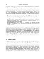
, as the coordinates, a three-dimensional stress space
can be constructed. This stress representation is known as the Haigh-Westergaard stress space,
Fig. 19.4.
3
1
Cos
J
2
−1
(s ,s ,s )
3
1
2
3
1
σ
N(p,p,p)

ρ
ξ
O
σ
2
σ
Hydrostatic axis
deviatoric plane
P( , , )
σ
σ
σ
1
2
3
Figure 19.4: Haigh-Westergaard Stress Space
18 The decomposition of a stress state into a hydrostatic, pδ
ij
and deviatoric s
ij
stress components
can be geometrically represented in this space. Considering an arbitrary stress state OP starting from
O(0, 0, 0) and ending at P(σ
1
,σ
2
,σ
3
), the vector OP can be decomposed into two components ON and
NP. The former is along the direction of the unit vector (1

√
3, 1/
√
3, 1/
√
3), and NP⊥ON.
19 Vector ON represents the hydrostatic component of the stress state, and axis Oξ is called the hy-
drostatic axis ξ, and every point on this axis has σ
1
= σ
2
= σ
3
= p,or
ξ =
√
3p (19.40)
Victor Saouma Mechanics of Materials II
Draft
19.4 Plastic Yield Conditions (Classical Models) 7
20 Vector NP represents the deviatoric component of the stress state (s
1
,s
2
,s
3
) and is perpendicular
to the ξ axis. Any plane perpendicular to the hydrostatic axis is called the deviatoric plane and is
expressed as
1

√
3
(σ
1
+ σ
2
+ σ
3
)=ξ (19.41)
and the particular plane which passes through the origin is called the π plane and is represented by
ξ = 0. Any plane containing the hydrostatic axis is called a meridian plane. The vector NP lies in a
meridian plane and has
ρ =

s
2
1
+ s
2
2
+ s
2
3
=

2J
2
(19.42)
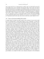
21 The projection of NP and the coordinate axes σ
i

on a deviatoric plane is shown in Fig. 19.5. The
σ
’
2
σ
3
’
120
0
120
0
120
0
P’
θ
N’
σ
’
1
Figure 19.5: Stress on a Deviatoric Plane
projection of N

P

of NP on this plane makes an angle θ with the axis σ

1
.
cos 3θ =
3

√
3
2
J
3
J
3/2
2
(19.43)
22 The three new variables ξ,ρ and θ can all be expressed in terms of the principal stresses through their
invariants. Hence, the general state of stress can be expressed either in terms of (σ
1
,σ
2
,σ
3
), or (ξ, ρ, θ).
For 0 ≤ θ ≤ π/3, and σ
1
≥ σ
2
≥ σ
3
,wehave



σ
1
σ

2
σ
3



=



p
p
p



+
2
√
3

J
2



cos θ
cos(θ −2π/3)
cos(θ +2π/3)




(19.44-a)
=



ξ
ξ
ξ



+

2
3
ρ



cos θ
cos(θ −2π/3)
cos(θ +2π/3)



(19.44-b)
(19.44-c)
19.4.2 Hydrostatic Pressure Independent Models

Adapted from (Chen and Zhang 1990)
23 For hydrostatic pressure independent yield surfaces (such as for steel), their meridians are straigth
lines parallel to the hydrostatic axis. Hence, shearing stress must be the major cause of yielding for
Victor Saouma Mechanics of Materials II
Draft
8 3D PLASTICITY
this type of materials. Since it is the magnitude of the shear stress that is important, and not its
direction, it follows that the elastic-plastic behavior in tension and in compression should be equivalent
for hydorstatic-pressure independent materials (such as steel). Hence, the cross-sectional shapes for this
kind of materials will have six-fold symmetry, and ρ
t
= ρ
c
.
19.4.2.1 Tresca
24 Tresca criterion postulates that yielding occurs when the maximum shear stress reaches a limiting
value k.
max

1
2
|σ
1
− σ
2
|,
1
2
|σ
2

− σ
3
|,
1
2
|σ
3
− σ
1
|

= k
(19.45)
from uniaxial tension test, we determine that k = σ
y
/2 and from pure shear test k = τ
y
. Hence, in
Tresca, tensile strength and shear strength are related by
σ
y
=2τ
y
(19.46)
25 Tresca’s criterion can also be represented as
2

J
2
sin


θ +
π
3

− σ
y
=0 for 0≤ θ ≤
π
3
(19.47)
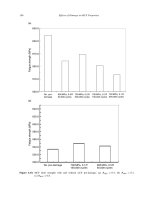
26 Tresca is on, Fig. 19.6:
Planeπ
σ
σ
3
σ
1
2
ξ
ρ
ρ
0
ξ
ρ
σ
1
’
ρ
0

σ
y
σ
2
−σ
y
−σ
y
σ
1
σ
τ
σ
3
σ
’
2
’
Figure 19.6: Tresca Criterion
• σ
1
σ
2
σ
3
space represented by an infinitly long regular hexagonal cylinder.
Victor Saouma Mechanics of Materials II
Draft
19.4 Plastic Yield Conditions (Classical Models) 9
• π (Deviatoric) Plane, the yield criterion is

ρ =2

J
2
=
σ
y
√
2sin

θ +
π
3

for 0 ≤ θ ≤
π
3
(19.48)
a regular hexagon with six singular corners.
• Meridian plane: a straight line parallel to the ξ axis.
• σ
1
σ
2
sub-space (with σ
3
= 0) an irregular hexagon. Note that in the σ
1
≥ 0,σ
2

≤ 0 the yield
criterion is
σ
1
− σ
2
= σ
y
(19.49)
• στ sub-space (with σ
3
= 0) is an ellipse

σ
σ
y

2
+

τ
τ
y

2
= 1 (19.50)
27 The Tresca criterion is the first one proposed, used mostly for elastic-plastic problems. However,
because of the singular corners, it causes numerous problems in numerical analysis.
19.4.2.2 von Mises
28 There are two different physical interpretation for the von Mises criteria postulate:

1. Material will yield when the distorsional (shear) energy reaches the same critical value as for yield
as in uniaxial tension.
F (J
2
)=J
2
− k
2
= 0 (19.51)
=

(σ
1
− σ
2
)
2
+(σ
2
− σ
3
)
2
+(σ
1
− σ
3
)
2
2

− σ
y
= 0 (19.52)
2. ρ, or the octahedral shear stress (CHECK) τ
oct
, the distance of the corresponding stress point
from the hydrostatic axis, ξ is constant and equal to:
ρ
0
= τ
y
√
2 (19.53)
29 Using Eq. 19.52, and from the uniaxial test, k is equal to k = σ
y
/
√
3, and from pure shear test k = τ
y
.
Hence, in von Mises, tensile strength and shear strength are related by
σ
y
=
√
3τ
y
(19.54)
Hence, we can rewrite Eq. 19.51 as
f(J

2
)=J
2
−
σ
2
y
3
= 0 (19.55)
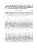
30 von Mises is on, Fig. ??:
• σ
1
σ
2
σ
3
space represented by an infinitly long regular circular cylinder.
• π (Deviatoric) Plane, the yield criterion is
ρ =

2
3
σ
y
(19.56)
a circle.
Victor Saouma Mechanics of Materials II
Draft
10 3D PLASTICITY
π Plane

1
σ
3
σ
2
σ
ξ
ρ
ρ
0
ξ
ρ
σ
1
’
ρ
0
σ
τ
σ
2
σ
’
2
σ
’
3
σ
1
x

y
Figure 19.7: von Mises Criterion
• Meridian plane: a straight line parallel to the ξ axis.
• σ
1
σ
2
sub-space (with σ
3
= 0) an ellipse
σ
2
1
+ σ
2
2
− σ
1
σ
2
= σ
2
y
(19.57)
• στ sub-space (with σ
3
= 0) is an ellipse

σ
σ

y

2
+

τ
τ
y

2
= 1 (19.58-a)
Note that whereas this equation is similar to the corresponding one for Tresca, Eq. 19.50, the
difference is in the relationships between σ
y
and τ
y
.
19.4.3 Hydrostatic Pressure Dependent Models
31 Pressure sensitive frictional materials (such as soil, rock, concrete) need to consider the effects of both
the first and second stress invariants. frictional materials such as concrete.
32 The cross-sections of a yield surface are the intersection curves between the yield surface and the
deviatoric plane (ρ, θ) which is perpendicular to the hydrostatic axis ξ and with ξ = constant. The
cross-sectional shapes of this yield surface will have threefold symmetry, Fig. 19.8.
33 The meridians of a yield surface are the intersection curves between the surface and a meridian plane
(ξ,ρ) which contains the hydrostatic axis. The meridian plane with θ = 0 is the tensile meridian,and
passes through the uniaxial tensile yield point. The meridian plane with θ = π/3isthecompressive
meridian and passes through the uniaxial compression yield point.
34 The radius of a yield surface on the tensile meridian is ρ
t
, and on the compressive meridian is ρ

c
.
Victor Saouma Mechanics of Materials II
Draft
19.4 Plastic Yield Conditions (Classical Models) 11
σ
’
1
σ
’
2
σ
3
’
ρ
ρ
ρ
c
t
θ
DEVIATORIC PLANE
ρ
ξ
MERIDIAN PLANE
Tensile Meridian
Compressive Meridian
θ=0
θ=π/3
Figure 19.8: Pressure Dependent Yield Surfaces
19.4.3.1 Rankine

35 The Rankine criterion postulates that yielding occur when the maximum principal stress reaches the
tensile strength.
σ
1
= σ
y
; σ
2
= σ
y
; σ
3
= σ
y
;
(19.59)
36 Rankine is on, Fig. 19.9:
• σ
1
σ
2
σ
3
space represented by XXX
• π (Deviatoric) Plane, the yield criterion is

ρ
t
=
1

√
2
(
√
3σ
Y
− ξ)
ρ
c
=
√
2(
√
3σ
y
− ξ)
(19.60)
a regular triangle.
• Meridian plane: Two straight lines which intersect the ξ axis ξ
y
=
√
3σ
y
• σ
1
σ
2
sub-space (with σ
3

= 0) two straight lines.

σ +1 = σ
y
σ
2
= σ
y
(19.61)
• στ sub-space (with σ
3
= 0) is a parabola
σ
σ
y
+

τ
σ
y

2
= 1 (19.62-a)
19.4.3.2 Mohr-Coulomb
37 The Mohr-Coulomb criteria can be considered as an extension of the Tresca criterion. The maximum
shear stress is a constant plus a function of the normal stress acting on the same plane.
|τ| = c − σ tan φ
(19.63)
Victor Saouma Mechanics of Materials II
Draft

12 3D PLASTICITY
c Cot
π Plane
3
1
σ
2
σ
ξ
ρ
σ
Φ
σ
1
’
σ
2
σ
t
σ
t
σ
t
σ
’
2
σ
’
3
σ

1
ξ
ρ
ρ
ρ
cy
ty
θ=0
θ=π/3
σ
τ
Figure 19.9: Rankine Criterion
where c is the cohesion, and φ the angle of internal friction.
38 Both c and φ are material properties which can be calibrated from uniaxial tensile and uniaxail
compressive tests.

σ
t
=
2c cos φ
1+sin φ
σ
c
=
2c cos φ
1−sin φ
(19.64)
39 In terms of invariants, the Mohr-Coulomb criteria can be expressed as:
1
3

I
1
sin φ +

J
2
sin

θ +
π
3

+

J
2
3
cos

θ +
π
3

sin φ − c cos φ =0 for 0≤ θ ≤
π
3
(19.65)
40 Mohr-Coulomb is on, Fig. 19.10:
• σ
1

σ
2
σ
3
space represented by a conical yield surface whose normal section at any point is an
irregular hexagon.
• π (Deviatoric) Plane, the cross-section of the surface is an irregular hexagon.
• Meridian plane: Two straight lines which intersect the ξ axis ξ
y
=2
√
3c/ tan φ, and the two
characteristic lengths of the surface on the deviatoric and meridian planes are

ρ
t
=
2
√
6c cos φ−2
√
2ξ sin φ
3+sin φ
ρ
c
=
2
√
6c cos φ−2
√

2ξ sin φ
3−sin φ
(19.66)
Victor Saouma Mechanics of Materials II
Draft
19.4 Plastic Yield Conditions (Classical Models) 13
c Cot
π Plane
3
2
1
σ
σ
ξ
ρ
σ
Φ
σ
1
’
ρ
ty
ρ
cy
σ
t
σ
t
σ
1

σ
2
−σ
c
σ
t
−σ
c
σ
’
2
σ
’
3
ξ
ρ
σ
θ=0
θ=π/3
ρ
cy
ρ
ty
τ
Figure 19.10: Mohr-Coulomb Criterion
• σ
1
σ
2
sub-space (with σ

3
= 0) the surface is an irregular hexagon. In the quarter σ
1
≥ 0,σ
2
≤ 0,
of the plane, the criterios is
mσ
1
− σ
2
= σ
c
(19.67)
where
m =
σ
c
σ
t
=
1+sinφ
1 − sin φ
(19.68)
• στ sub-space (with σ
3
= 0) is an ellipse

σ +
m−1

2m
σ
c
m+1
2m
σ
c

2
+

τ
√
m
2m
σ
c

2
(19.69-a)
19.4.3.3 Drucker-Prager
41 The Drucker-Prager postulates is a simple extension of the von Mises criterion to include the effect
of hydrostatic pressure on the yielding of the materials through I
1
F (I
1
,J
2
)=αI
1

+ J
2
− k
(19.70)
The strength parameters α and k can be determined from the uni axial tension and compression tests

σ
t
=
√
3k
1+
√
3α
σ
c
=
√
3k
1−
√
3α
(19.71)
Victor Saouma Mechanics of Materials II
Draft
14 3D PLASTICITY
or

α =
m−1

√
3(m+1)
k =
2σ
c
√
3(m+1)
(19.72)
42 Drucker-Prager is on, Fig. 19.11:
c Cot
π Plane
1
σ
3
Φ
2
σ
σ
ξ
ρ
σ
1
’
ρ
0
σ
2
σ
1
σ

t
σ
’
3
σ
’
2
ξ
ρ
y
x
σ
τ
−σ
c
Figure 19.11: Drucker-Prager Criterion
• σ
1
σ
2
σ
3
space represented by a circular cone.
• π (Deviatoric) Plane, the cross-section of the surface is a circle of radius ρ.
ρ =
√
2k −
√
6αξ (19.73)
• Meridian plane: The meridians of the surface are straight lines which intersect with the ξ axis

at ξ
y
= k/
√
3α.
• σ
1
σ
2
sub-space (with σ
3
= 0) the surface is an ellipse

x +
6
√
2kα
1−12α
2
√
6k
1−12α
2

2
+


y
√

2k
√
1−12α
2


2
(19.74)
where
x =
1
√
2
(σ
1
+ σ
2
) (19.75-a)
y =
1
√
2
(σ
2
− σ
1
) (19.75-b)
Victor Saouma Mechanics of Materials II
Draft
19.5 Plastic Potential 15

• στ sub-space (with σ
3
= 0) is also an ellipse

σ +
3kα
1−3α
2
√
3k
1−3α
2

2
+

τ
k
√
1−3α
2

2
= 1 (19.76-a)
43 In order to make the Drucker-Prager circle coincide with the Mohr-Coulomb hexagon at any section
Outer

α =
2sinφ
√

3(3−sin φ)
k =
6c cos φ
√
3(3−sin φ)
(19.77-a)
Inner

α =
2sinφ
√
3(3+sin φ)
k =
6c cos φ
√
3(3+sin φ)
(19.77-b)
19.5 Plastic Potential
44 Once a material yields, it exhibits permanent deformations through the generation of plastic strains.
According to the flow theory of plasticity, the rate of generation of these plastic strains is governed by the
flow rule. In order to define the direction of the plastic flow (which in turn determines the magnitudes
of the plastic strain components), it must be assumed that a scalar plastic potential function Q exists
such that Q = Q(σ
p
,ε
p
).
45 In the case of an associated flow rule, Q = F , and in the case of a non-associated flow rule, Q = F .
Since the plastic potential function helps define the plastic strain rate, it is often advantageous to define
a non-associated flow rule in order to control the amount of plastic strain generated by the plasticity

formulation. For example, when modeling plain concrete, excess plastic strains may lead to excess
dilatancy (too much volume expansion) which is undesirable. The plastic potential function can be
formulated to decrease the plastic strain rate, producing better results.
19.6 Plastic Flow Rule
46 We have established a yield criterion. When the stress is inside the yield surface, it is elastic, Hooke’s
law is applicable, strains are recoverable, and there is no dissipation of energy. However, when the load
on the structure pushes the stress tensor to be beyond the yield surface, the stress tensor locks up on
the yield surface, and the structure deforms plastically (if the material exhibits hardening as opposed
to elastic-perfectly plastic response, then the yield surface expands or moves with the stress point still
on the yield surface). At this point, the crucial question is what will be direction of the plastic flow
(that is the relative magnitude of the components of ε
P
. This question is addressed by the flow rule,
or normality rule.
47 We will assume that the direction of the plastic flow is given by a unit vector m, thus the incremental
plastic strain is written as
˙

p
=
˙
λ
p
∂Q
∂σ

m
p
(19.78)
where

˙
λ
p
is the plastic multiplier which scales the unit vector m
p
, in the direction of the plastic flow
evolution, to give the actual plastic strain in the material. Note analogy with Eq. 18.42.
Victor Saouma Mechanics of Materials II
Draft
16 3D PLASTICITY
48 We now must determine m, it is clearly a function of the stress state, and for convenience we represent
this vector as the gradient of a scalar potential Q which itself is a function of of the stresses
m =
∂Q
∂σ
= 
∂Q
∂σ
11
∂Q
∂σ
22
∂Q
∂σ
33
∂Q
∂σ
12
∂Q
∂σ

23
∂Q
∂σ
31

T
(19.79)
where Q is called the plastic flow potential and is yet to be defined. Hence, the direction of plastic
flow is always perpendicular to the plastic potential function.
49 We have two cases
Non-Associated Flow when F
p
= Q
p
which corresponds to the general case.
Associated Flow when when F
p
= Q
p
which is a special case. This gives rise to the Associated flow
rule
˙

p
=
˙
λ
p
∂F
p

∂σ
(19.80)
In this context, the difficulty in determining the normal of a yield surface with a sharp corner
should be noted.
50 The incremental plastic work (irrecoverable) is given by
dW
P
= σ·
˙
ε
P
(19.81)
which can be rewritten as
dW
P
= σ·λm (19.82)
51 Hence, the evolution of the stress state σ is given by the stress rate relation,
˙
σ
= E
o
:(
˙
 −
˙

p
)
(19.83)
19.7 Post-Yielding

19.7.1 Kuhn-Tucker Conditions
52 In the elastic regime, the yield function F must remain negative, and the rate of plastic multiplier
˙
λ
p
is zero. On the other hand, during plastic flow the yield function must be equal to zero while the rate
of plastic multiplier is positive.

plastic loading :
˙
F
p
=0;
˙
λ
p
> 0
elastic (un)loading :
˙
F
p
< 0;
˙
λ
p
=0
(19.84)
53 Hence, both cases can be simultaneously covered by the loading-unloading conditions called Kuhn-
Tucker conditions
˙

F
p
≤ 0,
˙
λ
p
≥ 0and
˙
F
p
˙
λ
p
=0
(19.85)
Victor Saouma Mechanics of Materials II
Draft
19.7 Post-Yielding 17
19.7.2 Hardening Rules
54 A hardening rule describes a specific relationship between the subsequent yield stress σ
y
of a material
and the plastic deformation accumulated during prior loadings.
55 We define a hardening parameter or plastic internal variable, which is often denoted by κ.
κ = ε
p
=

√
dε

p
dε
p
Equivalent Plastic Strain (19.86-a)
κ = W
p
=

σdε
p
Plastic Work (19.86-b)
κ = ε
p
=

dε
p
Plastic Strain (19.86-c)
56 A hardening rule expresses the relationship of the subsequent yield stress σ
y
, tangent modulus E
t
and plastic modulus E
p
with the hardening parameter κ.
19.7.2.1 Isotropic Hardening
57 In isotropic hardening, the yield surface simply increases in size but maintains its original shape.
Hence, the the progressively increasing yield stresses under both tension and compression loadings are
always the same.
|σ| = |σ(κ)| (19.87)

19.7.2.2 Kinematic Hardening
58 In kinematic hardening, the initial yield surface is translated to a new location in stress space without
change in size or shape. Hence, the difference between the yield stresses under tension loading and under
compression loading remains constant. If we denote by σ
t
y
and σ
c
y
the yield stress under tension and
compression respectively, then
σ
t
y
(κ) − σ
c
y
(κ)=2σ
y0
(19.88)
or alternatively
|σ −c(κ)| = σ
y0
(19.89)
where c(κ) represents the track of the elastic center and satisfies c(0) = 0.
59 Kinematic hardening accounts for the Baushinger effect, Fig. 16.2.
19.7.3 Consistency Condition
60 Fig. 19.12 illustrates the elastic d
e
and plastic d

p
strain increments for a given stress increment dσ.
Unloading always follows the initial elastic stiffness E
o
. The material experiences plastic loading once
the stress state exceeds the yield surface. Further loading results in the development of plastic strains
and stresses. However, the total stress state cannot exceed the yield surface. Thus, during plastic flow
the stress must remain on the yield surface, and hence the time derivative of the yield function must
vanish whenever and this limit is enforced through the consistency condition,
d
dt
F
p
(σ, ε
p
,κ)=
d
dt
F
p
(σ, λ,κ) = 0 (19.90)
or
∂F
p
∂σ


n
p
:

˙
σ +
∂F
p
∂λ
p

−H
p
:
˙
λ
p
+
∂F
p
∂κ
∂κ
∂λ
:
˙
λ
p
= 0 (19.91)
Victor Saouma Mechanics of Materials II
Draft
18 3D PLASTICITY
d
ε
d

ε
e
E
o
E
o
d
ε
e
E
o
d
ε
p
ε
σ
σ
d = :
Figure 19.12: Elastic and plastic strain increments
Ignoring the last term, this relation simplifies if the normal to the yield surface n
p
and the hardening
parameter H
p
are substituted, such that
˙
F
p
= n
p

:
˙
σ −H
p
˙
λ
p
=0
(19.92)
61 The consistency condition states that during persistent plastic flow the stresses remain on the yield
surface (since the rate of change of the yield function must be equal to zero).
62 An expression for the plastic multiplier
˙
λ
p
can be attained by the combination of the simplified
consistency condition Eq. 19.92 with the stress rate Eq. 19.83 and the flow rule Eq. 19.78:
˙
F
p
= n : E
o
:(
˙
 −
˙

p

˙

λ
p
m
p
)

 
˙
σ
−H
p
˙
λ
p
=0
˙
λ
p
=
n
p
: E
o
:
˙

H
p
+ n
p

: E
o
: m
p
≥ 0 (19.93)
63 The hardening parameter H
p
, defined above as H
p
= −∂F
p
/∂λ
p
, provides insight into the state of
the material in the plastic regime depending upon its sign:



hardening : H
p
> 0
perfect plasticity : H
p
=0
softening : H
p
< 0
(19.94)
19.8 Elasto-Plastic Stiffness Relation
64 Substituting the plastic multiplier expression of Eq. 19.93 into the stress rate expression Eq. 19.83

results in the following expression relating the stress and strain rate:
˙
σ = E
o
:

˙
 − m
p
:
n
p
: E
o
: m
p
H
p
+ n
p
: E
o
: m
p
:
˙


(19.95-a)
˙

σ =

E
o
−
E
o
: m
p
⊗ n
p
: E
o
H
p
+ n
p
: E
o
: m
p

:
˙
 (19.95-b)
Victor Saouma Mechanics of Materials II
Draft
19.9 †Case Study: J
2
Plasticity/von Mises Plasticity 19

from which the elastoplastic tangent operator may be identified as
E
p
= E
o
−
E
o
: m
p
⊗ n
p
: E
o
H
p
+ n
p
: E
o
: m
p
(19.96)
19.9 †Case Study: J
2
Plasticity/von Mises Plasticity
65 For J
2
plasticity or von Mises plasticity, our stress function is perfectly plastic. Recall perfectly plastic
materials have a total modulus of elasticity (E

T
) which is equivalent to zero. We will deal now with
deviatoric stress and strain for the J
2
plasticity stress function.
1. Yield function:
F (s)=
1
2
s : s −
1
3
σ
2
y
= 0 (19.97)
2. Flow rate (associated):
˙
e
p
=
˙
λ
∂Q
p
∂s
=
˙
λ
∂F

∂s
=
˙
λs (19.98)
3. Consistency condition (
˙
F = 0):
˙
F =
∂F
∂s
:
˙
s +
∂F
∂q
:
˙
q = 0 (19.99)
since
˙
q = 0 in perfect plasticity, the second term drops out and
˙
F becomes
˙
F = s :
˙
s = 0 (19.100)
Recall that
˙

s =2G :
˙
e
e
=2G :[
˙
e −
˙
e
p
] (19.101)
finally substituting
˙
e
p
in
˙
s =2G :[
˙
e −
˙
λs] (19.102)
substituting
˙
s back into (19.100)
˙
F =2Gs :[
˙
e −
˙

λm] = 0 (19.103)
and solving for
˙
λ
˙
λ =
s :
˙

s : s
(19.104)
4. Tangential stress-strain relation(deviatoric):
˙
s =2G :[
˙
e −
s :
˙
e
s : s
s] (19.105)
then by factoring
˙
e out
˙
s =2G :[I
4
−
s ⊗ s
s : s

]:
˙
e (19.106)
Now we have the simplified expression
˙
s = G
ep
:
˙
e (19.107)
where
G
ep
=2G :[I
4
−
s ⊗ s
s : s
] (19.108)
is the 4th order elastoplastic shear modulus tensor which relates deviatoric stress rate to deviatoric
strain rate.
Victor Saouma Mechanics of Materials II
Draft
20 3D PLASTICITY
5. Solving for E
ep
in order to relate regular stress and strain rates:
Volumetric response in purely elastic
tr (
˙

σ)=3Ktr (
˙
) (19.109)
altogether
˙
σ =
1
3
tr (
˙
σ):I
2
+
˙
s (19.110)
˙
σ = Ktr (
˙
):I
2
+ G
ep
:
˙
e (19.111)
˙
σ = Ktr (
˙
):I
2

+ G
ep
:[
˙
 −
1
3
tr (
˙
):I
2
] (19.112)
˙
σ = Ktr (
˙
):I
2
+ G
ep
:
˙
 −
1
3
tr (
˙
)G
ep
: I
2

(19.113)
˙
σ = Ktr (
˙
):I
2
−
2
3
Gtr (
˙
)I
2
+ G
ep
:
˙
 (19.114)
˙
σ = KI
2
⊗ I
2
:
˙
 −
2
3
GI
2

⊗ I
2
:
˙
 + G
ep
:
˙
 (19.115)
and finally we have recovered the stress-strain relationship
˙
σ =[[K −
2
3
G]I
2
⊗ I
2
+ G
ep
]:
˙
 (19.116)
where the elastoplastic material tensor is
E
ep
=[[K −
2
3
G]I

2
⊗ I
2
+ G
ep
] (19.117)
19.9.1 Isotropic Hardening/Softening(J
2
− plasticity)
66 In isotropic hardening/softening the yield surface may shrink (softening) or expand (hardening)
uniformly (see figure 19.13).
s
1
s
2
s
3
n+1
n+1
(Hardening)
F = 0 for
p
n
F = 0 for
(Perfectly Plastic)
H = 0
(Softening)
F = 0 for
H < 0
p

p
H > 0
Figure 19.13: Isotropic Hardening/Softening
1. Yield function for linear strain hardening/softening:
F (s,
p
eff
)=
1
2
s : s −
1
3
(σ
o
y
+ E
p

p
eff
)
2
= 0 (19.118)
Victor Saouma Mechanics of Materials II
Draft
19.9 †Case Study: J
2
Plasticity/von Mises Plasticity 21
2. Consistency condition:

˙
F =
∂F
∂s
:
˙
s +
∂F
∂q
:
∂
˙
q
∂
˙
λ
˙
λ = 0 (19.119)
from which we solve the plastic multiplier
˙
λ =
2Gs :
˙
e
2Gs : s +
2E
p
3
(σ
o

y
+ E
p

p
eff
)

2
3
s : s
(19.120)
3. Tangential stress-strain relation(deviatoric):
˙
s = G
ep
:
˙
e (19.121)
where
G
ep
=2G[I
4
−
2Gs ⊗ s
Gs : s +
2E
p
3

(σ
o
y
+ E
p

p
eff
)

2
3
s : s
] (19.122)
67 Note that isotropic hardening/softening is a poor representation of plastic behavior under cyclic
loading because of the Bauschinger effect.
19.9.2 Kinematic Hardening/Softening(J
2
− plasticity)
68 Kinematic hardening/softening, developed by Prager [1956], involves a shift of the origin of the yield
surface (see figure 19.14). Here, kinematic hardening/softening captures the Bauschinger effect in a more
realistic manner than the isotropic hardening/ softening.
s
2
s
3
s
1
F
n+2

= 0
F
n+1
= 0
F
n
= 0
O
R
P
S
Q
Figure 19.14: Kinematic Hardening/Softening
1. Yield function:
F (s, α)=
1
2
(s − α):(s − α) −
1
3
σ
2
y
= 0 (19.123)
2. Consistency condition (plastic multiplier):
˙
λ =
2G(s − α):
˙
e

(s − α):(s − α)[2G + C]
(19.124)
Victor Saouma Mechanics of Materials II
Draft
22 3D PLASTICITY
where
C = E
p
(19.125)
and C is related to α, the backstress, by
˙
α = C
˙
e =
˙
λC(s − α) (19.126)
For perfectly plastic behavior C =0andα =0.
3. Tangential stress-strain relation (deviatoric):
˙
s = G
ep
:
˙
e (19.127)
where
G
ep
=2G[I
4
−

2G(s − α) ⊗ (s − α)
(s − α):(s − α)[2G + C]
] (19.128)
19.10 Computer Implementation
Written by Eric Hansen
SUBROUTINE pd_strain(Outfid,Logfid,Pstfid,Lclfid)
! PD_STRAIN - Strain controlled parabolic Drucker-Prager model
!
! Variables required
!
! Outfid = Output file ID
! Logfid = Log file ID
! Pstfid = Post file ID
! Lclfid = Localization file ID
!
! Variables returned = none
!
! Subroutine called by
!
! p_drucker.f90 = Parabolic Drucker-Rrager model
!
! Functions/subroutines called
!
! alloc8.f90 = Allocate memory space in array Kmn
! el_ten1.f90 = Construct 4th order elastic stiffness tensor
!
! Variable definition
!
! Eo_ten = Elastic stiffness tensor
! Et_ten = Continuum tangent stiffness tensor

! alpha = Inverse damage-effect tensor
! alpha_bar = Damage-effect tensor
! phi_inc = Inverse integrity tensor for each load increment
! tr_sig = Trial stress tensor
! tr_eps = Trial strain tensor
! phibar_inc = Integrity tensor for current load increment
! w_ten = Square root inverse integrity tensor
! wbar_ten = Square root integrity tensor
! y_hat_pr = Principal values of conjugate tensile forces
!=========================================================================
IMPLICIT NONE
!
! Define interface with subroutine alloc8
!
INTERFACE
SUBROUTINE alloc8(Logfid,nrows,ncols,ptr)
IMPLICIT NONE
Victor Saouma Mechanics of Materials II
Draft
19.10 Computer Implementation 23
INTEGER,INTENT(IN) :: Logfid,nrows,ncols
DOUBLEPRECISION,POINTER,DIMENSION(:,:) :: ptr
END SUBROUTINE
END INTERFACE
!
! Define interface with C subroutines
!
INTERFACE
SUBROUTINE newline [C,ALIAS:’_newline’] (fid)
INTEGER fid [REFERENCE]

END SUBROUTINE newline
END INTERFACE
INTERFACE
SUBROUTINE tab [C,ALIAS:’_tab’] (fid)
INTEGER fid [REFERENCE]
END SUBROUTINE tab
END INTERFACE
INTERFACE
SUBROUTINE wrtchar [C,ALIAS:’_wrtchar’] (fid, stg_len, string)
INTEGER fid [REFERENCE]
INTEGER stg_len [REFERENCE]
CHARACTER*80 string [REFERENCE]
END SUBROUTINE wrtchar
END INTERFACE
INTERFACE
SUBROUTINE wrtint [C,ALIAS:’_wrtint’] (fid, param)
INTEGER fid [REFERENCE]
INTEGER param [REFERENCE]
END SUBROUTINE wrtint
END INTERFACE
INTERFACE
SUBROUTINE wrtreal [C,ALIAS:’_wrtreal’] (fid, param)
INTEGER fid [REFERENCE]
DOUBLEPRECISION param [REFERENCE]
END SUBROUTINE wrtreal
END INTERFACE
INTERFACE
SUBROUTINE wrtexp [C,ALIAS:’_wrtexp’] (fid, param)
INTEGER fid [REFERENCE]
DOUBLEPRECISION param [REFERENCE]

END SUBROUTINE wrtexp
END INTERFACE
INTERFACE
SUBROUTINE close_file [C,ALIAS:’_close_file’] (fid)
INTEGER fid [REFERENCE]
END SUBROUTINE close_file
END INTERFACE
!
! External function declaration
!
DOUBLEPRECISION,EXTERNAL :: pd_yield
DOUBLEPRECISION,EXTERNAL :: pd_limit_kp
DOUBLEPRECISION,EXTERNAL :: pd_limit_cp
DOUBLEPRECISION,EXTERNAL :: contract22
DOUBLEPRECISION,EXTERNAL :: firstinv
DOUBLEPRECISION,EXTERNAL :: pd_det_hp
!
! Pointer declaration/ Common pointer block
!
Victor Saouma Mechanics of Materials II
Draft
24 3D PLASTICITY
DOUBLEPRECISION,POINTER,DIMENSION(:,:) :: ptstrain
DOUBLEPRECISION,POINTER,DIMENSION(:,:) :: ptstress
COMMON /pointers/ ptstrain,ptstress
DOUBLEPRECISION,POINTER,DIMENSION(:,:) :: ptIDstrs
DOUBLEPRECISION,POINTER,DIMENSION(:,:) :: ptIDstrn
COMMON /pointerID/ ptIDstrs,ptIDstrn
!
! New pointer declaration

!
DOUBLEPRECISION,POINTER,DIMENSION(:,:) :: pthist1
DOUBLEPRECISION,POINTER,DIMENSION(:,:) :: pthist2
COMMON /pointers1/ pthist1,pthist2
DOUBLEPRECISION,POINTER,DIMENSION(:,:) :: ptmixed1
COMMON /ptrsmix/ ptmixed1
DOUBLEPRECISION,POINTER,DIMENSION(:,:) :: ptplasstn
COMMON /pointerplas/ ptplasstn
!
! Common variables
!
INTEGER :: mtype,ninc1,ninc2
INTEGER :: nstress,nstrain,ctype
COMMON /control/ mtype,ninc1,ninc2,nstress,nstrain,ctype
DOUBLEPRECISION :: young,pois
COMMON /material/ young,pois
DOUBLEPRECISION :: fpc_dp,fpt_dp,ko_dp,co_dp
COMMON /drucker/ fpc_dp,fpt_dp,ko_dp,co_dp
INTEGER :: lclflg,lclplane
COMMON /qanalysis/ lclflg,lclplane
INTEGER :: pstpleps,psteff
COMMON /printpst/ pstpleps,psteff
!
! Local Variable Type Declaration
!
INTEGER,INTENT(IN) :: Outfid,Logfid,Pstfid,Lclfid
DOUBLEPRECISION,ALLOCATABLE,DIMENSION(:,:,:,:) :: Eo_ten,Et_ten
DOUBLEPRECISION,ALLOCATABLE,DIMENSION(:,:,:) :: plastic_eps,t_plastic_eps
DOUBLEPRECISION,ALLOCATABLE,DIMENSION(:,:) :: eps_dot,old_eps
DOUBLEPRECISION,ALLOCATABLE,DIMENSION(:,:) :: tr_eps,tr_eps_e,tr_sig

DOUBLEPRECISION,ALLOCATABLE,DIMENSION(:,:) :: sig_dot,old_sig,NR_sig
DOUBLEPRECISION,ALLOCATABLE,DIMENSION(:,:) :: np_mat,mp_mat,barnp_mat,barmp_mat
DOUBLEPRECISION,ALLOCATABLE,DIMENSION(:,:) :: iter_peps,d_plas_eps
DOUBLEPRECISION,ALLOCATABLE,DIMENSION(:,:) :: iden
DOUBLEPRECISION,ALLOCATABLE,DIMENSION(:,:) :: dlam_deps
DOUBLEPRECISION,ALLOCATABLE,DIMENSION(:,:) :: temp_Es
DOUBLEPRECISION,ALLOCATABLE,DIMENSION(:,:) :: eps_inc
DOUBLEPRECISION,ALLOCATABLE,DIMENSION(:) :: sig_inc
DOUBLEPRECISION,ALLOCATABLE,DIMENSION(:) :: residl,resideps
DOUBLEPRECISION,ALLOCATABLE,DIMENSION(:) :: jnk1,jnk2
DOUBLEPRECISION,ALLOCATABLE,DIMENSION(:,:,:) :: local_data1
INTEGER,ALLOCATABLE,DIMENSION(:) :: local_data2
DOUBLEPRECISION :: fail_ep,dlam_ep_in
DOUBLEPRECISION :: limit_ep,limit_ep_k,limit_ep_c
DOUBLEPRECISION :: I1,beta,alpha
DOUBLEPRECISION :: determ
Victor Saouma Mechanics of Materials II