Information Theory, Inference, and Learning Algorithms phần 6 pptx
Bạn đang xem bản rút gọn của tài liệu. Xem và tải ngay bản đầy đủ của tài liệu tại đây (1.02 MB, 64 trang )
Copyright Cambridge University Press 2003. On-screen viewing permitted. Printing not permitted. />You can buy this book for 30 pounds or $50. See for links.
22.5: Further exercises 309
Exercises where maximum likelihood and MAP have difficulties
Exercise 22.14.
[2 ]
This exercise explores the idea that maximizing a proba-
bility density is a poor way to find a point that is representative of
the density. Consider a Gaussian distribution in a k-dimensional space,
P (w) = (1/
√
2π σ
W
)
k
exp(−
k
1
w
2
i
/2σ
2
W
). Show that nearly all of the
probability mass of a Gaussian is in a thin shell of radius r =
√
kσ
W
and of thickness proportional to r/
√
k. For example, in 1000 dimen-
sions, 90% of the mass of a Gaussian with σ
W
= 1 is in a shell of radius
31.6 and thickness 2.8. However, the probability density at the origin is
e
k/2
10
217
times bigger than the density at this shell where most of
the probability mass is.
Now consider two Gaussian densities in 1000 dimensions that differ in
radius σ
W
by just 1%, and that contain equal total probability mass.
Show that the maximum probability density is greater at the centre of
the Gaussian with smaller σ
W
by a factor of ∼exp(0.01k) 20000.
In ill-posed problems, a typical posterior distribution is often a weighted
superposition of Gaussians with varying means and standard deviations,
so the true posterior has a skew peak, with the maximum of the prob-
ability density located near the mean of the Gaussian distribution that
has the smallest standard deviation, not the Gaussian with the greatest
weight.
Exercise 22.15.
[3 ]
The seven scientists. N datapoints {x
n
} are drawn from
N distributions, all of which are Gaussian with a common mean µ but
with different unknown standard deviations σ
n
. What are the maximum
likelihood parameters µ, {σ
n
} given the data? For example, seven
-30 -20 -10 0 10 20
A B C D-G
Scientist x
n
A −27.020
B 3.570
C 8.191
D 9.898
E 9.603
F 9.945
G 10.056
Figure 22.9. Seven measurements
{x
n
} of a parameter µ by seven
scientists each having his own
noise-level σ
n
.
scientists (A, B, C, D, E, F, G) with wildly-differing experimental skills
measure µ. You expect some of them to do accurate work (i.e., to have
small σ
n
), and some of them to turn in wildly inaccurate answers (i.e.,
to have enormous σ
n
). Figure 22.9 shows their seven results. What is
µ, and how reliable is each scientist?
I hope you agree that, intuitively, it looks pretty certain that A and B
are both inept measurers, that D–G are better, and that the true value
of µ is somewhere close to 10. But what does maximizing the likelihood
tell you?
Exercise 22.16.
[3 ]
Problems with MAP method. A collection of widgets i =
1, . . . , k have a property called ‘wodge’, w
i
, which we measure, wid-
get by widget, in noisy experiments with a known noise level σ
ν
= 1.0.
Our model for these quantities is that they come from a Gaussian prior
P (w
i
|α) = Normal(0,
1
/
α), where α = 1/σ
2
W
is not known. Our prior for
this variance is flat over log σ
W
from σ
W
= 0.1 to σ
W
= 10.
Scenario 1. Suppose four widgets have been measured and give the fol-
lowing data: {d
1
, d
2
, d
3
, d
4
} = {2.2, −2.2, 2.8, −2.8}. We are interested
in inferring the wodges of these four widgets.
(a) Find the values of w and α that maximize the posterior probability
P (w, log α |d).
(b) Marginalize over α and find the posterior probability density of w
given the data. [Integration skills required. See MacKay (1999a) for
solution.] Find maxima of P (w |d). [Answer: two maxima – one at
w
MP
= {1.8, −1.8, 2.2, −2.2}, with error bars on all four parameters
Copyright Cambridge University Press 2003. On-screen viewing permitted. Printing not permitted. />You can buy this book for 30 pounds or $50. See for links.
310 22 — Maximum Likelihood and Clustering
(obtained from Gaussian approximation to the posterior) ±0.9; and
one at w
MP
= {0.03, −0.03, 0.04, −0.04} with error bars ±0.1.]
Scenario 2. Suppose in addition to the four measurements above we are
now informed that there are four more widgets that have been measured
with a much less accurate instrument, having σ
ν
= 100.0. Thus we now
have both well-determined and ill-determined parameters, as in a typical
ill-posed problem. The data from these measurements were a string of
uninformative values, {d
5
, d
6
, d
7
, d
8
} = {100, −100, 100, −100}.
We are again asked to infer the wodges of the widgets. Intuitively, our
inferences about the well-measured widgets should be negligibly affected
by this vacuous information about the poorly-measured widgets. But
what happens to the MAP method?
(a) Find the values of w and α that maximize the posterior probability
P (w, log α |d).
(b) Find maxima of P(w |d). [Answer: only one maximum, w
MP
=
{0.03, −0.03, 0.03, −0.03, 0.0001, −0.0001, 0.0001, −0.0001}, with
error bars on all eight parameters ±0.11.]
22.6 Solutions
Solution to exercise 22.5 (p.302). Figure 22.10 shows a contour plot of the
0 1 2 3 54
0
1
2
3
5
4
Figure 22.10. The likelihood as a
function of µ
1
and µ
2
.
likelihood function for the 32 data points. The peaks are pretty-near centred
on the points (1, 5) and (5, 1), and are pretty-near circular in their contours.
The width of each of the peaks is a standard deviation of σ/
√
16 = 1/4. The
peaks are roughly Gaussian in shape.
Solution to exercise 22.12 (p.307). The log likelihood is:
ln P ({x
(n)
}|w) = −N ln Z(w) +
n
k
w
k
f
k
(x
(n)
). (22.37)
∂
∂w
k
ln P ({x
(n)
}|w) = −N
∂
∂w
k
ln Z(w) +
n
f
k
(x). (22.38)
Now, the fun part is what happens when we differentiate the log of the nor-
malizing constant:
∂
∂w
k
ln Z(w) =
1
Z(w)
x
∂
∂w
k
exp
k
w
k
f
k
(x)
=
1
Z(w)
x
exp
k
w
k
f
k
(x)
f
k
(x) =
x
P (x |w)f
k
(x), (22.39)
so
∂
∂w
k
ln P ({x
(n)
}|w) = −N
x
P (x |w)f
k
(x) +
n
f
k
(x), (22.40)
and at the maximum of the likelihood,
x
P (x |w
ML
)f
k
(x) =
1
N
n
f
k
(x
(n)
). (22.41)
Copyright Cambridge University Press 2003. On-screen viewing permitted. Printing not permitted. />You can buy this book for 30 pounds or $50. See for links.
23
Useful Probability Distributions
0
0.05
0.1
0.15
0.2
0.25
0.3
0 1 2 3 4 5 6 7 8 9 10
1e-06
1e-05
0.0001
0.001
0.01
0.1
1
0 1 2 3 4 5 6 7 8 9 10
r
Figure 23.1. The binomial
distribution P (r |f = 0.3, N =10),
on a linear scale (top) and a
logarithmic scale (bottom).
In Bayesian data modelling, there’s a small collection of probability distribu-
tions that come up again and again. The purpose of this chapter is to intro-
duce these distributions so that they won’t be intimidating when encountered
in combat situations.
There is no need to memorize any of them, except perhaps the Gaussian;
if a distribution is important enough, it will memorize itself, and otherwise, it
can easily be looked up.
23.1 Distributions over integers
Binomial, Poisson, exponential
We already encountered the binomial distribution and the Poisson distribution
on page 2.
The binomial distribution for an integer r with parameters f (the bias,
f ∈ [0, 1]) and N (the number of trials) is:
P (r |f, N ) =
N
r
f
r
(1 −f)
N−r
r ∈ {0, 1, 2, . . . , N}. (23.1)
The binomial distribution arises, for example, when we flip a bent coin,
with bias f, N times, and observe the number of heads, r.
The Poisson distribution with parameter λ > 0 is:
P (r |λ) = e
−λ
λ
r
r!
r ∈ {0, 1, 2, . . .}. (23.2)
The Poisson distribution arises, for example, when we count the number of
photons r that arrive in a pixel during a fixed interval, given that the mean
intensity on the pixel corresponds to an average number of photons λ.
0
0.05
0.1
0.15
0.2
0.25
0 5 10 15
1e-07
1e-06
1e-05
0.0001
0.001
0.01
0.1
1
0 5 10 15
r
Figure 23.2. The Poisson
distribution P (r |λ =2.7), on a
linear scale (top) and a
logarithmic scale (bottom).
The exponential distribution on integers,,
P (r |f ) = f
r
(1 −f) r ∈ (0, 1, 2, . . . , ∞), (23.3)
arises in waiting problems. How long will you have to wait until a six is rolled,
if a fair six-sided dice is rolled? Answer: the probability distribution of the
number of rolls, r, is exponential over integers with parameter f = 5/6. The
distribution may also be written
P (r |f ) = (1 −f ) e
−λr
r ∈ (0, 1, 2, . . . , ∞), (23.4)
where λ = ln(1/f).
311
Copyright Cambridge University Press 2003. On-screen viewing permitted. Printing not permitted. />You can buy this book for 30 pounds or $50. See for links.
312 23 — Useful Probability Distributions
23.2 Distributions over unbounded real numbers
Gaussian, Student, Cauchy, biexponential, inverse-cosh.
The Gaussian distribution or normal distribution with mean µ and standard
deviation σ is
P (x |µ, σ) =
1
Z
exp
−
(x −µ)
2
2σ
2
x ∈ (−∞, ∞), (23.5)
where
Z =
√
2πσ
2
. (23.6)
It is sometimes useful to work with the quantity τ ≡ 1/σ
2
, which is called the
precision parameter of the Gaussian.
A sample z from a standard univariate Gaussian can be generated by
computing
z = cos(2πu
1
)
2 ln(1/u
2
), (23.7)
where u
1
and u
2
are uniformly distributed in (0, 1). A second sample z
2
=
sin(2πu
1
)
2 ln(1/u
2
), independent of the first, can then be obtained for free.
The Gaussian distribution is widely used and often asserted to be a very
common distribution in the real world, but I am sceptical about this asser-
tion. Yes, unimodal distributions may be common; but a Gaussian is a spe-
cial, rather extreme, unimodal distribution. It has very light tails: the log-
probability-density decreases quadratically. The typical deviation of x from µ
is σ, but the respective probabilities that x deviates from µ by more than 2σ,
3σ, 4σ, and 5σ, are 0.046, 0.003, 6 ×10
−5
, and 6 ×10
−7
. In my experience,
deviations from a mean four or five times greater than the typical deviation
may be rare, but not as rare as 6 ×10
−5
! I therefore urge caution in the use of
Gaussian distributions: if a variable that is modelled with a Gaussian actually
has a heavier-tailed distribution, the rest of the model will contort itself to
reduce the deviations of the outliers, like a sheet of paper being crushed by a
rubber band.
Exercise 23.1.
[1 ]
Pick a variable that is supposedly bell-shaped in probability
distribution, gather data, and make a plot of the variable’s empirical
distribution. Show the distribution as a histogram on a log scale and
investigate whether the tails are well-modelled by a Gaussian distribu-
tion. [One example of a variable to study is the amplitude of an audio
signal.]
One distribution with heavier tails than a Gaussian is a mixture of Gaus-
sians. A mixture of two Gaussians, for example, is defined by two means,
two standard deviations, and two mixing coefficients π
1
and π
2
, satisfying
π
1
+ π
2
= 1, π
i
≥ 0.
P (x |µ
1
, σ
1
, π
1
, µ
2
, σ
2
, π
2
) =
π
1
√
2πσ
1
exp
−
(x−µ
1
)
2
2σ
2
1
+
π
2
√
2πσ
2
exp
−
(x−µ
2
)
2
2σ
2
2
.
If we take an appropriately weighted mixture of an infinite number of
Gaussians, all having mean µ, we obtain a Student-t distribution,
P (x |µ, s, n) =
1
Z
1
(1 + (x − µ)
2
/(ns
2
))
(n+1)/2
, (23.8)
where
0
0.1
0.2
0.3
0.4
0.5
-2 0 2 4 6 8
0.0001
0.001
0.01
0.1
-2 0 2 4 6 8
Figure 23.3. Three unimodal
distributions. Two Student
distributions, with parameters
(m, s) = (1, 1) (heavy line) (a
Cauchy distribution) and (2, 4)
(light line), and a Gaussian
distribution with mean µ = 3 and
standard deviation σ = 3 (dashed
line), shown on linear vertical
scales (top) and logarithmic
vertical scales (bottom). Notice
that the heavy tails of the Cauchy
distribution are scarcely evident
in the upper ‘bell-shaped curve’.
Z =
√
πns
2
Γ(n/2)
Γ((n + 1)/2)
(23.9)
Copyright Cambridge University Press 2003. On-screen viewing permitted. Printing not permitted. />You can buy this book for 30 pounds or $50. See for links.
23.3: Distributions over positive real numbers 313
and n is called the number of degrees of freedom and Γ is the gamma function.
If n > 1 then the Student distribution (23.8) has a mean and that mean is
µ. If n > 2 the distribution also has a finite variance, σ
2
= ns
2
/(n − 2).
As n → ∞, the Student distribution approaches the normal distribution with
mean µ and standard deviation s. The Student distribution arises both in
classical statistics (as the sampling-theoretic distribution of certain statistics)
and in Bayesian inference (as the probability distribution of a variable coming
from a Gaussian distribution whose standard deviation we aren’t sure of).
In the special case n = 1, the Student distribution is called the Cauchy
distribution.
A distribution whose tails are intermediate in heaviness between Student
and Gaussian is the biexponential distribution,
P (x |µ, s) =
1
Z
exp
−
|x − µ|
s
x ∈ (−∞, ∞) (23.10)
where
Z = 2s. (23.11)
The inverse-cosh distribution
P (x |β) ∝
1
[cosh(βx)]
1/β
(23.12)
is a popular model in independent component analysis. In the limit of large β,
the probability distribution P(x |β) becomes a biexponential distribution. In
the limit β → 0 P (x |β) approaches a Gaussian with mean zero and variance
1/β.
23.3 Distributions over positive real numbers
Exponential, gamma, inverse-gamma, and log-normal.
The exponential distribution,
P (x |s) =
1
Z
exp
−
x
s
x ∈ (0, ∞), (23.13)
where
Z = s, (23.14)
arises in waiting problems. How long will you have to wait for a bus in Pois-
sonville, given that buses arrive independently at random with one every s
minutes on average? Answer: the probability distribution of your wait, x, is
exponential with mean s.
The gamma distribution is like a Gaussian distribution, except whereas the
Gaussian goes from −∞ to ∞, gamma distributions go from 0 to ∞. Just as
the Gaussian distribution has two parameters µ and σ which control the mean
and width of the distribution, the gamma distribution has two parameters. It
is the product of the one-parameter exponential distribution (23.13) with a
polynomial, x
c−1
. The exponent c in the polynomial is the second parameter.
P (x |s, c) = Γ(x; s, c) =
1
Z
x
s
c−1
exp
−
x
s
, 0 ≤ x < ∞ (23.15)
where
Z = Γ(c)s. (23.16)
Copyright Cambridge University Press 2003. On-screen viewing permitted. Printing not permitted. />You can buy this book for 30 pounds or $50. See for links.
314 23 — Useful Probability Distributions
0
0.1
0.2
0.3
0.4
0.5
0.6
0.7
0.8
0.9
1
0 2 4 6 8 10
0
0.1
0.2
0.3
0.4
0.5
0.6
0.7
0.8
-4 -2 0 2 4
0.0001
0.001
0.01
0.1
1
0 2 4 6 8 10
0.0001
0.001
0.01
0.1
-4 -2 0 2 4
x l = ln x
Figure 23.4. Two gamma
distributions, with parameters
(s, c) = (1, 3) (heavy lines) and
10, 0.3 (light lines), shown on
linear vertical scales (top) and
logarithmic vertical scales
(bottom); and shown as a
function of x on the left (23.15)
and l = ln x on the right (23.18).
This is a simple peaked distribution with mean sc and variance s
2
c.
It is often natural to represent a positive real variable x in terms of its
logarithm l = ln x. The probability density of l is
P (l) = P (x(l))
∂x
∂l
= P (x(l))x(l) (23.17)
=
1
Z
l
x(l)
s
c
exp
−
x(l)
s
, (23.18)
where
Z
l
= Γ(c). (23.19)
[The gamma distribution is named after its normalizing constant – an odd
convention, it seems to me!]
Figure 23.4 shows a couple of gamma distributions as a function of x and
of l. Notice that where the original gamma distribution (23.15) may have a
‘spike’ at x = 0, the distribution over l never has such a spike. The spike is
an artefact of a bad choice of basis.
In the limit sc = 1, c → 0, we obtain the noninformative prior for a scale
parameter, the 1/x prior. This improper prior is called noninformative because
it has no associated length scale, no characteristic value of x, so it prefers all
values of x equally. It is invariant under the reparameterization x = mx. If
we transform the 1/x probability density into a density over l = ln x we find
the latter density is uniform.
Exercise 23.2.
[1 ]
Imagine that we reparameterize a positive variable x in terms
of its cube root, u = x
1/3
. If the probability density of x is the improper
distribution 1/x, what is the probability density of u?
The gamma distribution is always a unimodal density over l = ln x, and,
as can be seen in the figures, it is asymmetric. If x has a gamma distribution,
and we decide to work in terms of the inverse of x, v = 1/x, we obtain a new
distribution, in which the density over l is flipped left-for-right: the probability
density of v is called an inverse-gamma distribution,
P (v |s, c) =
1
Z
v
1
sv
c+1
exp
−
1
sv
, 0 ≤ v < ∞ (23.20)
where
Z
v
= Γ(c)/s. (23.21)
Copyright Cambridge University Press 2003. On-screen viewing permitted. Printing not permitted. />You can buy this book for 30 pounds or $50. See for links.
23.4: Distributions over periodic variables 315
0
0.5
1
1.5
2
2.5
0 1 2 3
0
0.1
0.2
0.3
0.4
0.5
0.6
0.7
0.8
-4 -2 0 2 4
0.0001
0.001
0.01
0.1
1
0 1 2 3
0.0001
0.001
0.01
0.1
-4 -2 0 2 4
v ln v
Figure 23.5. Two inverse gamma
distributions, with parameters
(s, c) = (1, 3) (heavy lines) and
10, 0.3 (light lines), shown on
linear vertical scales (top) and
logarithmic vertical scales
(bottom); and shown as a
function of x on the left and
l = ln x on the right.
Gamma and inverse gamma distributions crop up in many inference prob-
lems in which a positive quantity is inferred from data. Examples include
inferring the variance of Gaussian noise from some noise samples, and infer-
ring the rate parameter of a Poisson distribution from the count.
Gamma distributions also arise naturally in the distributions of waiting
times between Poisson-distributed events. Given a Poisson process with rate
λ, the probability density of the arrival time x of the mth event is
λ(λx)
m−1
(m−1)!
e
−λx
. (23.22)
Log-normal distribution
Another distribution over a positive real number x is the log-normal distribu-
tion, which is the distribution that results when l = ln x has a normal distri-
bution. We define m to be the median value of x, and s to be the standard
deviation of ln x.
P (l |m, s) =
1
Z
exp
−
(l − ln m)
2
2s
2
l ∈ (−∞, ∞), (23.23)
where
Z =
√
2πs
2
, (23.24)
implies
P (x |m, s) =
1
x
exp
−
(ln x − ln m)
2
2s
2
x ∈ (0, ∞). (23.25)
0
0.05
0.1
0.15
0.2
0.25
0.3
0.35
0.4
0 1 2 3 4 5
0.0001
0.001
0.01
0.1
0 1 2 3 4 5
Figure 23.6. Two log-normal
distributions, with parameters
(m, s) = (3, 1.8) (heavy line) and
(3, 0.7) (light line), shown on
linear vertical scales (top) and
logarithmic vertical scales
(bottom). [Yes, they really do
have the same value of the
median, m = 3.]
23.4 Distributions over periodic variables
A periodic variable θ is a real number ∈ [0, 2π] having the property that θ = 0
and θ = 2π are equivalent.
A distribution that plays for periodic variables the role played by the Gaus-
sian distribution for real variables is the Von Mises distribution:
P (θ |µ, β) =
1
Z
exp (β cos(θ −µ)) θ ∈ (0, 2π). (23.26)
The normalizing constant is Z = 2πI
0
(β), where I
0
(x) is a modified Bessel
function.
Copyright Cambridge University Press 2003. On-screen viewing permitted. Printing not permitted. />You can buy this book for 30 pounds or $50. See for links.
316 23 — Useful Probability Distributions
A distribution that arises from Brownian diffusion around the circle is the
wrapped Gaussian distribution,
P (θ |µ, σ) =
∞
n=−∞
Normal(θ; (µ + 2πn), σ) θ ∈ (0, 2π). (23.27)
23.5 Distributions over probabilities
Beta distribution, Dirichlet distribution, entropic distribution
The beta distribution is a probability density over a variable p that is a prob-
0
1
2
3
4
5
0 0.25 0.5 0.75 1
0
0.1
0.2
0.3
0.4
0.5
0.6
-6 -4 -2 0 2 4 6
Figure 23.7. Three beta
distributions, with
(u
1
, u
2
) = (0.3, 1), (1.3, 1), and
(12, 2). The upper figure shows
P (p |u
1
, u
2
) as a function of p; the
lower shows the corresponding
density over the logit,
ln
p
1 − p
.
Notice how well-behaved the
densities are as a function of the
logit.
ability, p ∈ (0, 1):
P (p |u
1
, u
2
) =
1
Z(u
1
, u
2
)
p
u
1
−1
(1 −p)
u
2
−1
. (23.28)
The parameters u
1
, u
2
may take any positive value. The normalizing constant
is the beta function,
Z(u
1
, u
2
) =
Γ(u
1
)Γ(u
2
)
Γ(u
1
+ u
2
)
. (23.29)
Special cases include the uniform distribution – u
1
= 1, u
2
= 1; the Jeffreys
prior – u
1
= 0.5, u
2
= 0.5; and the improper Laplace prior – u
1
= 0, u
2
= 0. If
we transform the beta distribution to the corresponding density over the logit
l ≡ ln p/ (1 − p), we find it is always a pleasant bell-shaped density over l, while
the density over p may have singularities at p = 0 and p = 1 (figure 23.7).
More dimensions
The Dirichlet distribution is a density over an I-dimensional vector p whose
I components are positive and sum to 1. The beta distribution is a special
case of a Dirichlet distribution with I = 2. The Dirichlet distribution is
parameterized by a measure u (a vector with all coefficients u
i
> 0) which
I will write here as u = αm, where m is a normalized measure over the I
components (
m
i
= 1), and α is positive:
P (p |αm) =
1
Z(αm)
I
i=1
p
αm
i
−1
i
δ (
i
p
i
− 1) ≡ Dirichlet
(I)
(p |αm). (23.30)
The function δ(x) is the Dirac delta function, which restricts the distribution
to the simplex such that p is normalized, i.e.,
i
p
i
= 1. The normalizing
constant of the Dirichlet distribution is:
Z(αm) =
i
Γ(αm
i
) /Γ(α) . (23.31)
The vector m is the mean of the probability distribution:
Dirichlet
(I)
(p |αm) p d
I
p = m. (23.32)
When working with a probability vector p, it is often helpful to work in the
‘softmax basis’, in which, for example, a three-dimensional probability p =
(p
1
, p
2
, p
3
) is represented by three numbers a
1
, a
2
, a
3
satisfying a
1
+a
2
+a
3
= 0
and
p
i
=
1
Z
e
a
i
, where Z =
i
e
a
i
. (23.33)
This nonlinear transformation is analogous to the σ → ln σ transformation
for a scale variable and the logit transformation for a single probability, p →
Copyright Cambridge University Press 2003. On-screen viewing permitted. Printing not permitted. />You can buy this book for 30 pounds or $50. See for links.
23.5: Distributions over probabilities 317
u = (20, 10, 7) u = (0.2, 1, 2) u = (0.2, 0.3, 0.15)
-8
-4
0
4
8
-8 -4 0 4 8
-8
-4
0
4
8
-8 -4 0 4 8
-8
-4
0
4
8
-8 -4 0 4 8
Figure 23.8. Three Dirichlet
distributions over a
three-dimensional probability
vector (p
1
, p
2
, p
3
). The upper
figures show 1000 random draws
from each distribution, showing
the values of p
1
and p
2
on the two
axes. p
3
= 1 − (p
1
+ p
2
). The
triangle in the first figure is the
simplex of legal probability
distributions.
The lower figures show the same
points in the ‘softmax’ basis
(equation (23.33)). The two axes
show a
1
and a
2
. a
3
= −a
1
− a
2
.
ln
p
1−p
. In the softmax basis, the ugly minus-ones in the exponents in the
Dirichlet distribution (23.30) disappear, and the density is given by:
P (a |αm) ∝
1
Z(αm)
I
i=1
p
αm
i
i
δ (
i
a
i
) . (23.34)
The role of the parameter α can be characterized in two ways. First, α mea-
sures the sharpness of the distribution (figure 23.8); it measures how different
we expect typical samples p from the distribution to be from the mean m, just
as the precision τ =
1
/
σ
2
of a Gaussian measures how far samples stray from its
mean. A large value of α produces a distribution over p that is sharply peaked
around m. The effect of α in higher-dimensional situations can be visualized
by drawing a typical sample from the distribution Dirichlet
(I)
(p |αm), with
m set to the uniform vector m
i
=
1
/
I, and making a Zipf plot, that is, a ranked
plot of the values of the components p
i
. It is traditional to plot both p
i
(ver-
tical axis) and the rank (horizontal axis) on logarithmic scales so that power
law relationships appear as straight lines. Figure 23.9 shows these plots for a
single sample from ensembles with I = 100 and I = 1000 and with α from 0.1
to 1000. For large α, the plot is shallow with many components having simi-
lar values. For small α, typically one component p
i
receives an overwhelming
share of the probability, and of the small probability that remains to be shared
among the other components, another component p
i
receives a similarly large
share. In the limit as α goes to zero, the plot tends to an increasingly steep
power law.
I = 100
0.0001
0.001
0.01
0.1
1
1 10 100
0.1
1
10
100
1000
I = 1000
1e-05
0.0001
0.001
0.01
0.1
1
1 10 100 1000
0.1
1
10
100
1000
Figure 23.9. Zipf plots for random
samples from Dirichlet
distributions with various values
of α = 0.1 . . . 1000. For each value
of I = 100 or 1000 and each α,
one sample p from the Dirichlet
distribution was generated. The
Zipf plot shows the probabilities
p
i
, ranked by magnitude, versus
their rank.
Second, we can characterize the role of α in terms of the predictive dis-
tribution that results when we observe samples from p and obtain counts
F = (F
1
, F
2
, . . . , F
I
) of the possible outcomes. The value of α defines the
number of samples from p that are required in order that the data dominate
over the prior in predictions.
Exercise 23.3.
[3 ]
The Dirichlet distribution satisfies a nice additivity property.
Imagine that a biased six-sided die has two red faces and four blue faces.
The die is rolled N times and two Bayesians examine the outcomes in
order to infer the bias of the die and make predictions. One Bayesian
has access to the red/blue colour outcomes only, and he infers a two-
component probability vector (p
R
, p
B
). The other Bayesian has access
to each full outcome: he can see which of the six faces came up, and
he infers a six-component probability vector (p
1
, p
2
, p
3
, p
4
, p
5
, p
6
), where
Copyright Cambridge University Press 2003. On-screen viewing permitted. Printing not permitted. />You can buy this book for 30 pounds or $50. See for links.
318 23 — Useful Probability Distributions
p
R
= p
1
+ p
2
and p
B
= p
3
+ p
4
+ p
5
+ p
6
. Assuming that the sec-
ond Bayesian assigns a Dirichlet distribution to (p
1
, p
2
, p
3
, p
4
, p
5
, p
6
) with
hyperparameters (u
1
, u
2
, u
3
, u
4
, u
5
, u
6
), show that, in order for the first
Bayesian’s inferences to be consistent with those of the second Bayesian,
the first Bayesian’s prior should be a Dirichlet distribution with hyper-
parameters ((u
1
+ u
2
), (u
3
+ u
4
+ u
5
+ u
6
)).
Hint: a brute-force approach is to compute the integral P (p
R
, p
B
) =
d
6
p P (p |u) δ(p
R
− (p
1
+ p
2
)) δ(p
B
− (p
3
+ p
4
+ p
5
+ p
6
)). A cheaper
approach is to compute the predictive distributions, given arbitrary data
(F
1
, F
2
, F
3
, F
4
, F
5
, F
6
), and find the condition for the two predictive dis-
tributions to match for all data.
The entropic distribution for a probability vector p is sometimes used in
the ‘maximum entropy’ image reconstruction community.
P (p |α, m) =
1
Z(α, m)
exp[−αD
KL
(p||m)] δ(
i
p
i
− 1) , (23.35)
where m, the measure, is a positive vector, and D
KL
(p||m) =
i
p
i
log p
i
/m
i
.
Further reading
See (MacKay and Peto, 1995) for fun with Dirichlets.
23.6 Further exercises
Exercise 23.4.
[2 ]
N datapoints {x
n
} are drawn from a gamma distribution
P (x |s, c) = Γ(x; s, c) with unknown parameters s and c. What are the
maximum likelihood parameters s and c?
Copyright Cambridge University Press 2003. On-screen viewing permitted. Printing not permitted. />You can buy this book for 30 pounds or $50. See for links.
24
Exact Marginalization
How can we avoid the exponentially large cost of complete enumeration of
all hypotheses? Before we stoop to approximate methods, we explore two
approaches to exact marginalization: first, marginalization over continuous
variables (sometimes known as nuisance parameters) by doing integrals; and
second, summation over discrete variables by message-passing.
Exact marginalization over continuous parameters is a macho activity en-
joyed by those who are fluent in definite integration. This chapter uses gamma
distributions; as was explained in the previous chapter, gamma distributions
are a lot like Gaussian distributions, except that whereas the Gaussian goes
from −∞ to ∞, gamma distributions go from 0 to ∞.
24.1 Inferring the mean and variance of a Gaussian distribution
We discuss again the one-dimensional Gaussian distribution, parameterized
by a mean µ and a standard deviation σ:
P (x |µ, σ) =
1
√
2πσ
exp
−
(x − µ)
2
2σ
2
≡ Normal(x; µ, σ
2
). (24.1)
When inferring these parameters, we must specify their prior distribution.
The prior gives us the opportunity to include specific knowledge that we have
about µ and σ (from independent experiments, or on theoretical grounds, for
example). If we have no such knowledge, then we can construct an appropriate
prior that embodies our supposed ignorance. In section 21.2, we assumed a
uniform prior over the range of parameters plotted. If we wish to be able to
perform exact marginalizations, it may be useful to consider conjugate priors;
these are priors whose functional form combines naturally with the likelihood
such that the inferences have a convenient form.
Conjugate priors for µ and σ
The conjugate prior for a mean µ is a Gaussian: we introduce two ‘hy-
perparameters’, µ
0
and σ
µ
, which parameterize the prior on µ, and write
P (µ |µ
0
, σ
µ
) = Normal(µ; µ
0
, σ
µ
). In the limit µ
0
= 0, σ
µ
→ ∞, we obtain
the noninformative prior for a location parameter, the flat prior. This is
noninformative because it is invariant under the natural reparameterization
µ
= µ+ c. The prior P(µ) = const. is also an improper prior, that is, it is not
normalizable.
The conjugate prior for a standard deviation σ is a gamma distribution,
which has two parameters b
β
and c
β
. It is most convenient to define the prior
319
Copyright Cambridge University Press 2003. On-screen viewing permitted. Printing not permitted. />You can buy this book for 30 pounds or $50. See for links.
320 24 — Exact Marginalization
density of the inverse variance (the precision parameter) β = 1/σ
2
:
P (β) = Γ(β;b
β
, c
β
) =
1
Γ(c
β
)
β
c
β
−1
b
c
β
β
exp
−
β
b
β
, 0 ≤ β < ∞. (24.2)
This is a simple peaked distribution with mean b
β
c
β
and variance b
2
β
c
β
. In
the limit b
β
c
β
= 1, c
β
→ 0, we obtain the noninformative prior for a scale
parameter, the 1/σ prior. This is ‘noninformative’ because it is invariant
under the reparameterization σ
= cσ. The 1/σ prior is less strange-looking if
we examine the resulting density over ln σ, or ln β, which is flat. This is the Reminder: when we change
variables from σ to l(σ), a
one-to-one function of σ, the
probability density transforms
from P
σ
(σ) to
P
l
(l) = P
σ
(σ)
∂σ
∂l
.
Here, the Jacobian is
∂σ
∂ ln σ
= σ.
prior that expresses ignorance about σ by saying ‘well, it could be 10, or it
could be 1, or it could be 0.1, . . . ’ Scale variables such as σ are usually best
represented in terms of their logarithm. Again, this noninformative 1/σ prior
is improper.
In the following examples, I will use the improper noninformative priors
for µ and σ. Using improper priors is viewed as distasteful in some circles,
so let me excuse myself by saying it’s for the sake of readability; if I included
proper priors, the calculations could still be done but the key points would be
obscured by the flood of extra parameters.
Maximum likelihood and marginalization: σ
N
and σ
N−1
The task of inferring the mean and standard deviation of a Gaussian distribu-
tion from N samples is a familiar one, though maybe not everyone understands
the difference between the σ
N
and σ
N−1
buttons on their calculator. Let us
recap the formulae, then derive them.
Given data D = {x
n
}
N
n=1
, an ‘estimator’ of µ is
¯x ≡
N
n=1
x
n
/N, (24.3)
and two estimators of σ are:
σ
N
≡
N
n=1
(x
n
− ¯x)
2
N
and σ
N−1
≡
N
n=1
(x
n
− ¯x)
2
N − 1
. (24.4)
There are two principal paradigms for statistics: sampling theory and Bayesian
inference. In sampling theory (also known as ‘frequentist’ or orthodox statis-
tics), one invents estimators of quantities of interest and then chooses between
those estimators using some criterion measuring their sampling properties;
there is no clear principle for deciding which criterion to use to measure the
performance of an estimator; nor, for most criteria, is there any systematic
procedure for the construction of optimal estimators. In Bayesian inference,
in contrast, once we have made explicit all our assumptions about the model
and the data, our inferences are mechanical. Whatever question we wish to
pose, the rules of probability theory give a unique answer which consistently
takes into account all the given information. Human-designed estimators and
confidence intervals have no role in Bayesian inference; human input only en-
ters into the important tasks of designing the hypothesis space (that is, the
specification of the model and all its probability distributions), and figuring
out how to do the computations that implement inference in that space. The
answers to our questions are probability distributions over the quantities of
interest. We often find that the estimators of sampling theory emerge auto-
matically as modes or means of these posterior distributions when we choose
a simple hypothesis space and turn the handle of Bayesian inference.
Copyright Cambridge University Press 2003. On-screen viewing permitted. Printing not permitted. />You can buy this book for 30 pounds or $50. See for links.
24.1: Inferring the mean and variance of a Gaussian distribution 321
(a1)
0
0.5
1
1.5
2
0.2
0.4
0.6
0.8
1
0
0.01
0.02
0.03
0.04
0.05
0.06
mean
sigma
(a2)
0 0.5 1 1.5 2
0.1
0.2
0.3
0.4
0.5
0.6
0.7
0.8
0.9
1
mean
sigma
(c)
0
0.01
0.02
0.03
0.04
0.05
0.06
0.07
0.08
0.09
0.2 0.4 0.6 0.8 1 1.2 1.4 1.61.8 2
mu=1
mu=1.25
mu=1.5
(d)
0
0.01
0.02
0.03
0.04
0.05
0.06
0.07
0.08
0.09
0.2 0.4 0.6 0.8 1 1.2 1.4 1.61.8 2
P(sigma|D)
P(sigma|D,mu=1)
Figure 24.1. The likelihood
function for the parameters of a
Gaussian distribution, repeated
from figure 21.5.
(a1, a2) Surface plot and contour
plot of the log likelihood as a
function of µ and σ. The data set
of N = 5 points had mean ¯x = 1.0
and S
2
=
(x − ¯x)
2
= 1.0.
Notice that the maximum is skew
in σ. The two estimators of
standard deviation have values
σ
N
= 0.45 and σ
N−1
= 0.50.
(c) The posterior probability of σ
for various fixed values of µ
(shown as a density over ln σ).
(d) The posterior probability of σ,
P (σ |D), assuming a flat prior on
µ, obtained by projecting the
probability mass in (a) onto the σ
axis. The maximum of P(σ |D) is
at σ
N−1
. By contrast, the
maximum of P(σ |D, µ = ¯x) is at
σ
N
. (Both probabilities are shows
as densities over ln σ.)
In sampling theory, the estimators above can be motivated as follows. ¯x is
an unbiased estimator of µ which, out of all the possible unbiased estimators
of µ, has smallest variance (where this variance is computed by averaging over
an ensemble of imaginary experiments in which the data samples are assumed
to come from an unknown Gaussian distribution). The estimator (¯x, σ
N
) is the
maximum likelihood estimator for (µ, σ). The estimator σ
N
is biased, however:
the expectation of σ
N
, given σ, averaging over many imagined experiments, is
not σ.
Exercise 24.1.
[2, p.323]
Give an intuitive explanation why the estimator σ
N
is
biased.
This bias motivates the invention, in sampling theory, of σ
N−1
, which can be
shown to be an unbiased estimator. Or to be precise, it is σ
2
N−1
that is an
unbiased estimator of σ
2
.
We now look at some Bayesian inferences for this problem, assuming non-
informative priors for µ and σ. The emphasis is thus not on the priors, but
rather on (a) the likelihood function, and (b) the concept of marginalization.
The joint posterior probability of µ and σ is proportional to the likelihood
function illustrated by a contour plot in figure 24.1a. The log likelihood is:
ln P ({x
n
}
N
n=1
|µ, σ) = −N ln(
√
2πσ) −
n
(x
n
− µ)
2
/(2σ
2
), (24.5)
= −N ln(
√
2πσ) − [N(µ − ¯x)
2
+ S]/(2σ
2
), (24.6)
where S ≡
n
(x
n
− ¯x)
2
. Given the Gaussian model, the likelihood can be
expressed in terms of the two functions of the data ¯x and S, so these two
quantities are known as ‘sufficient statistics’. The posterior probability of µ
and σ is, using the improper priors:
P (µ, σ |{x
n
}
N
n=1
) =
P ({x
n
}
N
n=1
|µ, σ)P (µ, σ)
P ({x
n
}
N
n=1
)
(24.7)
=
1
(2πσ
2
)
N/2
exp
−
N(µ−¯x)
2
+S
2σ
2
1
σ
µ
1
σ
P ({x
n
}
N
n=1
)
. (24.8)
Copyright Cambridge University Press 2003. On-screen viewing permitted. Printing not permitted. />You can buy this book for 30 pounds or $50. See for links.
322 24 — Exact Marginalization
This function describes the answer to the question, ‘given the data, and the
noninformative priors, what might µ and σ be?’ It may be of interest to find
the parameter values that maximize the posterior probability, though it should
be emphasized that posterior probability maxima have no fundamental status
in Bayesian inference, since their location depends on the choice of basis. Here
we choose the basis (µ, ln σ), in which our prior is flat, so that the posterior
probability maximum coincides with the maximum of the likelihood. As we
saw in exercise 22.4 (p.302), the maximum likelihood solution for µ and ln σ
is {µ, σ}
ML
=
¯x, σ
N
=
S/N
.
There is more to the posterior distribution than just its mode. As can
be seen in figure 24.1a, the likelihood has a skew peak. As we increase σ,
the width of the conditional distribution of µ increases (figure 22.1b). And
if we fix µ to a sequence of values moving away from the sample mean ¯x, we
obtain a sequence of conditional distributions over σ whose maxima move to
increasing values of σ (figure 24.1c).
The posterior probability of µ given σ is
P (µ |{x
n
}
N
n=1
, σ) =
P ({x
n
}
N
n=1
|µ, σ)P (µ)
P ({x
n
}
N
n=1
|σ)
(24.9)
∝ exp(−N(µ − ¯x)
2
/(2σ
2
)) (24.10)
= Normal(µ; ¯x, σ
2
/N). (24.11)
We note the familiar σ/
√
N scaling of the error bars on µ.
Let us now ask the question ‘given the data, and the noninformative priors,
what might σ be?’ This question differs from the first one we asked in that we
are now not interested in µ. This parameter must therefore be marginalized
over. The posterior probability of σ is:
P (σ |{x
n
}
N
n=1
) =
P ({x
n
}
N
n=1
|σ)P (σ)
P ({x
n
}
N
n=1
)
. (24.12)
The data-dependent term P ({x
n
}
N
n=1
|σ) appeared earlier as the normalizing
constant in equation (24.9); one name for this quantity is the ‘evidence’, or
marginal likelihood, for σ. We obtain the evidence for σ by integrating out
µ; a noninformative prior P (µ) = constant is assumed; we call this constant
1/σ
µ
, so that we can think of the prior as a top-hat prior of width σ
µ
. The
Gaussian integral, P ({x
n
}
N
n=1
|σ) =
P ({x
n
}
N
n=1
|µ, σ)P (µ) dµ, yields:
ln P ({x
n
}
N
n=1
|σ) = −N ln(
√
2πσ) −
S
2σ
2
+ ln
√
2πσ/
√
N
σ
µ
. (24.13)
The first two terms are the best fit log likelihood (i.e., the log likelihood with
µ = ¯x). The last term is the log of the Occam factor which penalizes smaller
values of σ. (We will discuss Occam factors more in Chapter 28.) When we
differentiate the log evidence with respect to ln σ, to find the most probable
σ, the additional volume factor (σ/
√
N) shifts the maximum from σ
N
to
σ
N−1
=
S/(N −1). (24.14)
Intuitively, the denominator (N −1) counts the number of noise measurements
contained in the quantity S =
n
(x
n
−¯x)
2
. The sum contains N residuals
squared, but there are only (N −1) effective noise measurements because the
determination of one parameter µ from the data causes one dimension of noise
to be gobbled up in unavoidable overfitting. In the terminology of classical
Copyright Cambridge University Press 2003. On-screen viewing permitted. Printing not permitted. />You can buy this book for 30 pounds or $50. See for links.
24.2: Exercises 323
statistics, the Bayesian’s best guess for σ sets χ
2
(the measure of deviance
defined by χ
2
≡
n
(x
n
− ˆµ)
2
/ˆσ
2
) equal to the number of degrees of freedom,
N − 1.
Figure 24.1d shows the posterior probability of σ, which is proportional
to the marginal likelihood. This may be contrasted with the posterior prob-
ability of σ with µ fixed to its most probable value, ¯x = 1, which is shown in
figure 24.1c and d.
The final inference we might wish to make is ‘given the data, what is µ?’
Exercise 24.2.
[3 ]
Marginalize over σ and obtain the posterior marginal distri-
bution of µ, which is a Student-t distribution:
P (µ |D) ∝ 1/
N(µ − ¯x)
2
+ S
N/2
. (24.15)
Further reading
A bible of exact marginalization is Bretthorst’s (1988) book on Bayesian spec-
trum analysis and parameter estimation.
24.2 Exercises
Exercise 24.3.
[3 ]
[This exercise requires macho integration capabilities.] Give
a Bayesian solution to exercise 22.15 (p.309), where seven scientists of
varying capabilities have measured µ with personal noise levels σ
n
,
-30 -20 -10 0 10 20
A B C D-G
and we are interested in inferring µ. Let the prior on each σ
n
be a
broad prior, for example a gamma distribution with parameters (s, c) =
(10, 0.1). Find the posterior distribution of µ. Plot it, and explore its
properties for a variety of data sets such as the one given, and the data
set {x
n
} = {13.01, 7.39}.
[Hint: first find the posterior distribution of σ
n
given µ and x
n
,
P (σ
n
|x
n
, µ). Note that the normalizing constant for this inference is
P (x
n
|µ). Marginalize over σ
n
to find this normalizing constant, then
use Bayes’ theorem a second time to find P (µ |{x
n
}).]
24.3 Solutions
Solution to exercise 24.1 (p.321). 1. The data points are distributed with mean
squared deviation σ
2
about the true mean. 2. The sample mean is unlikely
to exactly equal the true mean. 3. The sample mean is the value of µ that
minimizes the sum squared deviation of the data points from µ. Any other
value of µ (in particular, the true value of µ) will have a larger value of the
sum-squared deviation that µ = ¯x.
So the expected mean squared deviation from the sample mean is neces-
sarily smaller than the mean squared deviation σ
2
about the true mean.
Copyright Cambridge University Press 2003. On-screen viewing permitted. Printing not permitted. />You can buy this book for 30 pounds or $50. See for links.
25
Exact Marginalization in Trellises
In this chapter we will discuss a few exact methods that are used in proba-
bilistic modelling. As an example we will discuss the task of decoding a linear
error-correcting code. We will see that inferences can be conducted most effi-
ciently by message-passing algorithms, which take advantage of the graphical
structure of the problem to avoid unnecessary duplication of computations
(see Chapter 16).
25.1 Decoding problems
A codeword t is selected from a linear (N, K) code C, and it is transmitted
over a noisy channel; the received signal is y. In this chapter we will assume
that the channel is a memoryless channel such as a Gaussian channel. Given
an assumed channel model P (y |t), there are two decoding problems.
The codeword decoding problem is the task of inferring which codeword
t was transmitted given the received signal.
The bitwise decoding problem is the task of inferring for each transmit-
ted bit t
n
how likely it is that that bit was a one rather than a zero.
As a concrete example, take the (7, 4) Hamming code. In Chapter 1, we
discussed the codeword decoding problem for that code, assuming a binary
symmetric channel. We didn’t discuss the bitwise decoding problem and we
didn’t discuss how to handle more general channel models such as a Gaussian
channel.
Solving the codeword decoding problem
By Bayes’ theorem, the posterior probability of the codeword t is
P (t |y) =
P (y |t)P (t)
P (y)
. (25.1)
Likelihood function. The first factor in the numerator, P(y |t), is the likeli-
hood of the codeword, which, for any memoryless channel, is a separable
function,
P (y |t) =
N
n=1
P (y
n
|t
n
). (25.2)
For example, if the channel is a Gaussian channel with transmissions ±x
and additive noise of standard deviation σ, then the probability density
324
Copyright Cambridge University Press 2003. On-screen viewing permitted. Printing not permitted. />You can buy this book for 30 pounds or $50. See for links.
25.1: Decoding problems 325
of the received signal y
n
in the two cases t
n
= 0, 1 is
P (y
n
|t
n
= 1) =
1
√
2πσ
2
exp
−
(y
n
−x)
2
2σ
2
(25.3)
P (y
n
|t
n
= 0) =
1
√
2πσ
2
exp
−
(y
n
+ x)
2
2σ
2
. (25.4)
From the point of view of decoding, all that matters is the likelihood
ratio, which for the case of the Gaussian channel is
P (y
n
|t
n
= 1)
P (y
n
|t
n
= 0)
= exp
2xy
n
σ
2
. (25.5)
Exercise 25.1.
[2 ]
Show that from the point of view of decoding, a Gaussian
channel is equivalent to a time-varying binary symmetric channel with
a known noise level f
n
which depends on n.
Prior. The second factor in the numerator is the prior probability of the
codeword, P(t), which is usually assumed to be uniform over all valid
codewords.
The denominator in (25.1) is the normalizing constant
P (y) =
t
P (y |t)P (t). (25.6)
The complete solution to the codeword decoding problem is a list of all
codewords and their probabilities as given by equation (25.1). Since the num-
ber of codewords in a linear code, 2
K
, is often very large, and since we are not
interested in knowing the detailed probabilities of all the codewords, we often
restrict attention to a simplified version of the codeword decoding problem.
The MAP codeword decoding problem is the task of identifying the
most probable codeword t given the received signal.
If the prior probability over codewords is uniform then this task is iden-
tical to the problem of maximum likelihood decoding, that is, identifying
the codeword that maximizes P (y |t).
Example: In Chapter 1, for the (7, 4) Hamming code and a binary symmetric
channel we discussed a method for deducing the most probable codeword from
the syndrome of the received signal, thus solving the MAP codeword decoding
problem for that case. We would like a more general solution.
The MAP codeword decoding problem can be solved in exponential time
(of order 2
K
) by searching through all codewords for the one that maximizes
P (y |t)P (t). But we are interested in methods that are more efficient than
this. In section 25.3, we will discuss an exact method known as the min–sum
algorithm which may be able to solve the codeword decoding problem more
efficiently; how much more efficiently depends on the properties of the code.
It is worth emphasizing that MAP codeword decoding for a general lin-
ear code is known to be NP-complete (which means in layman’s terms that
MAP codeword decoding has a complexity that scales exponentially with the
blocklength, unless there is a revolution in computer science). So restrict-
ing attention to the MAP decoding problem hasn’t necessarily made the task
much less challenging; it simply makes the answer briefer to report.
Copyright Cambridge University Press 2003. On-screen viewing permitted. Printing not permitted. />You can buy this book for 30 pounds or $50. See for links.
326 25 — Exact Marginalization in Trellises
Solving the bitwise decoding problem
Formally, the exact solution of the bitwise decoding problem is obtained from
equation (25.1) by marginalizing over the other bits.
P (t
n
|y) =
{t
n
: n
=n}
P (t |y). (25.7)
We can also write this marginal with the aid of a truth function
[S] that is
one if the proposition S is true and zero otherwise.
P (t
n
= 1 |y) =
t
P (t |y)
[t
n
= 1] (25.8)
P (t
n
= 0 |y) =
t
P (t |y)
[t
n
= 0]. (25.9)
Computing these marginal probabilities by an explicit sum over all codewords
t takes exponential time. But, for certain codes, the bitwise decoding problem
can be solved much more efficiently using the forward–backward algorithm.
We will describe this algorithm, which is an example of the sum–product
algorithm, in a moment. Both the min–sum algorithm and the sum–product
algorithm have widespread importance, and have been invented many times
in many fields.
25.2 Codes and trellises
In Chapters 1 and 11, we represented linear (N, K) codes in terms of their
generator matrices and their parity-check matrices. In the case of a systematic
block code, the first K transmitted bits in each block of size N are the source
bits, and the remaining M = N −K bits are the parity-check bits. This means
that the generator matrix of the code can be written
G
T
=
I
K
P
, (25.10)
and the parity-check matrix can be written
H =
P I
M
, (25.11)
where P is an M ×K matrix.
In this section we will study another representation of a linear code called a
trellis. The codes that these trellises represent will not in general be systematic
codes, but they can be mapped onto systematic codes if desired by a reordering
of the bits in a block.
(a)
Repetition code R
3
(b)
Simple parity code P
3
(c)
(7, 4) Hamming code
Figure 25.1. Examples of trellises.
Each edge in a trellis is labelled
by a zero (shown by a square) or
a one (shown by a cross).
Definition of a trellis
Our definition will be quite narrow. For a more comprehensive view of trellises,
the reader should consult Kschischang and Sorokine (1995).
A trellis is a graph consisting of nodes (also known as states or vertices) and
edges. The nodes are grouped into vertical slices called times, and the
times are ordered such that each edge connects a node in one time to
a node in a neighbouring time. Every edge is labelled with a symbol.
The leftmost and rightmost states contain only one node. Apart from
these two extreme nodes, all nodes in the trellis have at least one edge
connecting leftwards and at least one connecting rightwards.
Copyright Cambridge University Press 2003. On-screen viewing permitted. Printing not permitted. />You can buy this book for 30 pounds or $50. See for links.
25.3: Solving the decoding problems on a trellis 327
A trellis with N +1 times defines a code of blocklength N as follows: a
codeword is obtained by taking a path that crosses the trellis from left to right
and reading out the symbols on the edges that are traversed. Each valid path
through the trellis defines a codeword. We will number the leftmost time ‘time
0’ and the rightmost ‘time N’. We will number the leftmost state ‘state 0’
and the rightmost ‘state I’, where I is the total number of states (vertices) in
the trellis. The nth bit of the codeword is emitted as we move from time n−1
to time n.
The width of the trellis at a given time is the number of nodes in that
time. The maximal width of a trellis is what it sounds like.
A trellis is called a linear trellis if the code it defines is a linear code. We will
solely be concerned with linear trellises from now on, as nonlinear trellises are
much more complex beasts. For brevity, we will only discuss binary trellises,
that is, trellises whose edges are labelled with zeroes and ones. It is not hard
to generalize the methods that follow to q-ary trellises.
Figures 25.1(a–c) show the trellises corresponding to the repetition code
R
3
which has (N,K) = (3, 1); the parity code P
3
with (N, K) = (3, 2); and
the (7, 4) Hamming code.
Exercise 25.2.
[2 ]
Confirm that the sixteen codewords listed in table 1.14 are
generated by the trellis shown in figure 25.1c.
Observations about linear trellises
For any linear code the minimal trellis is the one that has the smallest number
of nodes. In a minimal trellis, each node has at most two edges entering it and
at most two edges leaving it. All nodes in a time have the same left degree as
each other and they have the same right degree as each other. The width is
always a power of two.
A minimal trellis for a linear (N, K) code cannot have a width greater than
2
K
since every node has at least one valid codeword through it, and there are
only 2
K
codewords. Furthermore, if we define M = N − K, the minimal
trellis’s width is everywhere less than 2
M
. This will be proved in section 25.4.
Notice that for the linear trellises in figure 25.1, all of which are minimal
trellises, K is the number of times a binary branch point is encountered as the
trellis is traversed from left to right or from right to left.
We will discuss the construction of trellises more in section 25.4. But we
now know enough to discuss the decoding problem.
25.3 Solving the decoding problems on a trellis
We can view the trellis of a linear code as giving a causal description of the
probabilistic process that gives rise to a codeword, with time flowing from left
to right. Each time a divergence is encountered, a random source (the source
of information bits for communication) determines which way we go.
At the receiving end, we receive a noisy version of the sequence of edge-
labels, and wish to infer which path was taken, or to be precise, (a) we want
to identify the most probable path in order to solve the codeword decoding
problem; and (b) we want to find the probability that the transmitted symbol
at time n was a zero or a one, to solve the bitwise decoding problem.
Example 25.3. Consider the case of a single transmission from the Hamming
(7, 4) trellis shown in figure 25.1c.
Copyright Cambridge University Press 2003. On-screen viewing permitted. Printing not permitted. />You can buy this book for 30 pounds or $50. See for links.
328 25 — Exact Marginalization in Trellises
t Likelihood Posterior probability
0000000 0.0275562 0.25
0001011 0.0001458 0.0013
0010111 0.0013122 0.012
0011100 0.0030618 0.027
0100110 0.0002268 0.0020
0101101 0.0000972 0.0009
0110001 0.0708588 0.63
0111010 0.0020412 0.018
1000101 0.0001458 0.0013
1001110 0.0000042 0.0000
1010010 0.0030618 0.027
1011001 0.0013122 0.012
1100011 0.0000972 0.0009
1101000 0.0002268 0.0020
1110100 0.0020412 0.018
1111111 0.0000108 0.0001
Figure 25.2. Posterior probabilities
over the sixteen codewords when
the received vector y has
normalized likelihoods
(0.1, 0.4, 0.9, 0.1, 0.1, 0.1, 0.3).
Let the normalized likelihoods be: (0.1, 0.4, 0.9, 0.1, 0.1, 0.1, 0.3). That is,
the ratios of the likelihoods are
P (y
1
|x
1
= 1)
P (y
1
|x
1
= 0)
=
0.1
0.9
,
P (y
2
|x
2
= 1)
P (y
2
|x
2
= 0)
=
0.4
0.6
, etc. (25.12)
How should this received signal be decoded?
1. If we threshold the likelihoods at 0.5 to turn the signal into a bi-
nary received vector, we have r = (0, 0, 1, 0, 0, 0, 0), which decodes,
using the decoder for the binary symmetric channel (Chapter 1), into
ˆ
t = (0, 0, 0, 0, 0, 0, 0).
This is not the optimal decoding procedure. Optimal inferences are
always obtained by using Bayes’ theorem.
2. We can find the posterior probability over codewords by explicit enu-
meration of all sixteen codewords. This posterior distribution is shown
in figure 25.2. Of course, we aren’t really interested in such brute-force
solutions, and the aim of this chapter is to understand algorithms for
getting the same information out in less than 2
K
computer time.
Examining the posterior probabilities, we notice that the most probable
codeword is actually the string t = 0110001. This is more than twice as
probable as the answer found by thresholding, 0000000.
Using the posterior probabilities shown in figure 25.2, we can also com-
pute the posterior marginal distributions of each of the bits. The result
is shown in figure 25.3. Notice that bits 1, 4, 5 and 6 are all quite con-
fidently inferred to be zero. The strengths of the posterior probabilities
for bits 2, 3, and 7 are not so great. ✷
In the above example, the MAP codeword is in agreement with the bitwise
decoding that is obtained by selecting the most probable state for each bit
using the posterior marginal distributions. But this is not always the case, as
the following exercise shows.
Copyright Cambridge University Press 2003. On-screen viewing permitted. Printing not permitted. />You can buy this book for 30 pounds or $50. See for links.
25.3: Solving the decoding problems on a trellis 329
n Likelihood Posterior marginals
P (y
n
|t
n
= 1) P (y
n
|t
n
= 0) P (t
n
= 1 |y) P (t
n
= 0 |y)
1 0.1 0.9 0.061 0.939
2 0.4 0.6 0.674 0.326
3 0.9 0.1 0.746 0.254
4 0.1 0.9 0.061 0.939
5 0.1 0.9 0.061 0.939
6 0.1 0.9 0.061 0.939
7 0.3 0.7 0.659 0.341
Figure 25.3. Marginal posterior
probabilities for the 7 bits under
the posterior distribution of
figure 25.2.
Exercise 25.4.
[2, p.333]
Find the most probable codeword in the case where
the normalized likelihood is (0.2, 0.2, 0.9, 0.2, 0.2, 0.2, 0.2). Also find or
estimate the marginal posterior probability for each of the seven bits,
and give the bit-by-bit decoding.
[Hint: concentrate on the few codewords that have the largest probabil-
ity.]
We now discuss how to use message passing on a code’s trellis to solve the
decoding problems.
The min–sum algorithm
The MAP codeword decoding problem can be solved using the min–sum al-
gorithm that was introduced in section 16.3. Each codeword of the code
corresponds to a path across the trellis. Just as the cost of a journey is the
sum of the costs of its constituent steps, the log likelihood of a codeword is
the sum of the bitwise log likelihoods. By convention, we flip the sign of the
log likelihood (which we would like to maximize) and talk in terms of a cost,
which we would like to minimize.
We associate with each edge a cost −log P (y
n
|t
n
), where t
n
is the trans-
mitted bit associated with that edge, and y
n
is the received symbol. The
min–sum algorithm presented in section 16.3 can then identify the most prob-
able codeword in a number of computer operations equal to the number of
edges in the trellis. This algorithm is also known as the Viterbi algorithm
(Viterbi, 1967).
The sum–product algorithm
To solve the bitwise decoding problem, we can make a small modification to
the min–sum algorithm, so that the messages passed through the trellis define
‘the probability of the data up to the current point’ instead of ‘the cost of the
best route to this point’. We replace the costs on the edges, −log P (y
n
|t
n
), by
the likelihoods themselves, P (y
n
|t
n
). We replace the min and sum operations
of the min–sum algorithm by a sum and product respectively.
Let i run over nodes/states, i = 0 be the label for the start state, P(i)
denote the set of states that are parents of state i, and w
ij
be the likelihood
associated with the edge from node j to node i. We define the forward-pass
messages α
i
by
α
0
= 1
Copyright Cambridge University Press 2003. On-screen viewing permitted. Printing not permitted. />You can buy this book for 30 pounds or $50. See for links.
330 25 — Exact Marginalization in Trellises
α
i
=
j∈P(i)
w
ij
α
j
. (25.13)
These messages can be computed sequentially from left to right.
Exercise 25.5.
[2 ]
Show that for a node i whose time-coordinate is n, α
i
is
proportional to the joint probability that the codeword’s path passed
through node i and that the first n received symbols were y
1
, . . . , y
n
.
The message α
I
computed at the end node of the trellis is proportional to the
marginal probability of the data.
Exercise 25.6.
[2 ]
What is the constant of proportionality? [Answer: 2
K
]
We define a second set of backward-pass messages β
i
in a similar manner.
Let node I be the end node.
β
I
= 1
β
j
=
i:j∈P(i)
w
ij
β
i
. (25.14)
These messages can be computed sequentially in a backward pass from right
to left.
Exercise 25.7.
[2 ]
Show that for a node i whose time-coordinate is n, β
i
is
proportional to the conditional probability, given that the codeword’s
path passed through node i, that the subsequent received symbols were
y
n+1
. . . y
N
.
Finally, to find the probability that the nth bit was a 1 or 0, we do two
summations of products of the forward and backward messages. Let i run over
nodes at time n and j run over nodes at time n − 1, and let t
ij
be the value
of t
n
associated with the trellis edge from node j to node i. For each value of
t = 0/1, we compute
r
(t)
n
=
i,j: j∈P(i), t
ij
=t
α
j
w
ij
β
i
. (25.15)
Then the posterior probability that t
n
was t = 0/1 is
P (t
n
= t |y) =
1
Z
r
(t)
n
, (25.16)
where the normalizing constant Z = r
(0)
n
+ r
(1)
n
should be identical to the final
forward message α
I
that was computed earlier.
Exercise 25.8.
[2 ]
Confirm that the above sum–product algorithm does com-
pute P (t
n
= t |y).
Other names for the sum–product algorithm presented here are ‘the forward–
backward algorithm’, ‘the BCJR algorithm’, and ‘belief propagation’.
Exercise 25.9.
[2, p.333]
A codeword of the simple parity code P
3
is transmitted,
and the received signal y has associated likelihoods shown in table 25.4.
n P (y
n
|t
n
)
t
n
= 0 t
n
= 1
1
1
/
4
1
/
2
2
1
/
2
1
/
4
3
1
/
8
1
/
2
Table 25.4. Bitwise likelihoods for
a codeword of P
3
.
Use the min–sum algorithm and the sum–product algorithm in the trellis
(figure 25.1) to solve the MAP codeword decoding problem and the
bitwise decoding problem. Confirm your answers by enumeration of
all codewords (000, 011, 110, 101). [Hint: use logs to base 2 and do
the min–sum computations by hand. When working the sum–product
algorithm by hand, you may find it helpful to use three colours of pen,
one for the αs, one for the ws, and one for the βs.]
Copyright Cambridge University Press 2003. On-screen viewing permitted. Printing not permitted. />You can buy this book for 30 pounds or $50. See for links.
25.4: More on trellises 331
25.4 More on trellises
We now discuss various ways of making the trellis of a code. You may safely
jump over this section.
The span of a codeword is the set of bits contained between the first bit in
the codeword that is non-zero, and the last bit that is non-zero, inclusive. We
can indicate the span of a codeword by a binary vector as shown in table 25.5.
Codeword 0000000 0001011 0100110 1100011 0101101
Span 0000000 0001111 0111110 1111111 0111111
Table 25.5. Some codewords and
their spans.
A generator matrix is in trellis-oriented form if the spans of the rows of the
generator matrix all start in different columns and the spans all end in different
columns.
How to make a trellis from a generator matrix
First, put the generator matrix into trellis-oriented form by row-manipulations
similar to Gaussian elimination. For example, our (7, 4) Hamming code can
be generated by
G =
1 0 0 0 1 0 1
0 1 0 0 1 1 0
0 0 1 0 1 1 1
0 0 0 1 0 1 1
(25.17)
but this matrix is not in trellis-oriented form – for example, rows 1, 3 and 4
all have spans that end in the same column. By subtracting lower rows from
upper rows, we can obtain an equivalent generator matrix (that is, one that
generates the same set of codewords) as follows:
G =
1 1 0 1 0 0 0
0 1 0 0 1 1 0
0 0 1 1 1 0 0
0 0 0 1 0 1 1
. (25.18)
Now, each row of the generator matrix can be thought of as defining an
(N, 1) subcode of the (N,K) code, that is, in this case, a code with two
codewords of length N = 7. For the first row, the code consists of the two
codewords 1101000 and 0000000. The subcode defined by the second row
consists of 0100110 and 0000000. It is easy to construct the minimal trellises
of these subcodes; they are shown in the left column of figure 25.6.
We build the trellis incrementally as shown in figure 25.6. We start with
the trellis corresponding to the subcode given by the first row of the generator
matrix. Then we add in one subcode at a time. The vertices within the span
of the new subcode are all duplicated. The edge symbols in the original trellis
are left unchanged and the edge symbols in the second part of the trellis are
flipped wherever the new subcode has a 1 and otherwise left alone.
Another (7, 4) Hamming code can be generated by
G =
1 1 1 0 0 0 0
0 1 1 1 1 0 0
0 0 1 0 1 1 0
0 0 0 1 1 1 1
. (25.19)
Copyright Cambridge University Press 2003. On-screen viewing permitted. Printing not permitted. />You can buy this book for 30 pounds or $50. See for links.
332 25 — Exact Marginalization in Trellises
+
=
+
=
+
=
Figure 25.6. Trellises for four
subcodes of the (7, 4) Hamming
code (left column), and the
sequence of trellises that are made
when constructing the trellis for
the (7, 4) Hamming code (right
column).
Each edge in a trellis is labelled
by a zero (shown by a square) or
a one (shown by a cross).
The (7, 4) Hamming code generated by this matrix differs by a permutation
of its bits from the code generated by the systematic matrix used in Chapter
1 and above. The parity-check matrix corresponding to this permutation is:
H =
1 0 1 0 1 0 1
0 1 1 0 0 1 1
0 0 0 1 1 1 1
. (25.20)
The trellis obtained from the permuted matrix G given in equation (25.19) is
shown in figure 25.7a. Notice that the number of nodes in this trellis is smaller
than the number of nodes in the previous trellis for the Hamming (7, 4) code
in figure 25.1c. We thus observe that rearranging the order of the codeword
bits can sometimes lead to smaller, simpler trellises.
(a)
(b)
Figure 25.7. Trellises for the
permuted (7, 4) Hamming code
generated from (a) the generator
matrix by the method of
figure 25.6; (b) the parity-check
matrix by the method on page
332.
Each edge in a trellis is labelled
by a zero (shown by a square) or
a one (shown by a cross).
Trellises from parity-check matrices
Another way of viewing the trellis is in terms of the syndrome. The syndrome
of a vector r is defined to be Hr, where H is the parity-check matrix. A vector
is only a codeword if its syndrome is zero. As we generate a codeword we can
describe the current state by the partial syndrome, that is, the product of
H with the codeword bits thus far generated. Each state in the trellis is a
partial syndrome at one time coordinate. The starting and ending states are
both constrained to be the zero syndrome. Each node in a state represents a
different possible value for the partial syndrome. Since H is an M ×N matrix,
where M = N −K, the syndrome is at most an M -bit vector. So we need at
most 2
M
nodes in each state. We can construct the trellis of a code from its
parity-check matrix by walking from each end, generating two trees of possible
syndrome sequences. The intersection of these two trees defines the trellis of
the code.
In the pictures we obtain from this construction, we can let the vertical
coordinate represent the syndrome. Then any horizontal edge is necessarily
associated with a zero bit (since only a non-zero bit changes the syndrome)
Copyright Cambridge University Press 2003. On-screen viewing permitted. Printing not permitted. />You can buy this book for 30 pounds or $50. See for links.
25.5: Solutions 333
and any non-horizontal edge is associated with a one bit. (Thus in this rep-
resentation we no longer need to label the edges in the trellis.) Figure 25.7b
shows the trellis corresponding to the parity-check matrix of equation (25.20).
25.5 Solutions
t Likelihood Posterior probability
0000000 0.026 0.3006
0001011 0.00041 0.0047
0010111 0.0037 0.0423
0011100 0.015 0.1691
0100110 0.00041 0.0047
0101101 0.00010 0.0012
0110001 0.015 0.1691
0111010 0.0037 0.0423
1000101 0.00041 0.0047
1001110 0.00010 0.0012
1010010 0.015 0.1691
1011001 0.0037 0.0423
1100011 0.00010 0.0012
1101000 0.00041 0.0047
1110100 0.0037 0.0423
1111111 0.000058 0.0007
Table 25.8. The posterior
probability over codewords for
exercise 25.4.
Solution to exercise 25.4 (p.329). The posterior probability over codewords is
shown in table 25.8. The most probable codeword is 0000000. The marginal
posterior probabilities of all seven bits are:
n Likelihood Posterior marginals
P (y
n
|t
n
= 1) P (y
n
|t
n
= 0) P (t
n
= 1 |y) P (t
n
= 0 |y)
1 0.2 0.8 0.266 0.734
2 0.2 0.8 0.266 0.734
3 0.9 0.1 0.677 0.323
4 0.2 0.8 0.266 0.734
5 0.2 0.8 0.266 0.734
6 0.2 0.8 0.266 0.734
7 0.2 0.8 0.266 0.734
So the bitwise decoding is 0010000, which is not actually a codeword.
Solution to exercise 25.9 (p.330). The MAP codeword is 101, and its like-
lihood is 1/8. The normalizing constant of the sum–product algorithm is
Z = α
I
=
3
/
16. The intermediate α
i
are (from left to right)
1
/
2,
1
/
4,
5
/
16,
4
/
16;
the intermediate β
i
are (from right to left),
1
/
2,
1
/
8,
9
/
32,
3
/
16. The bitwise
decoding is: P (t
1
= 1 |y) = 3/4; P (t
1
= 1 |y) = 1/4; P (t
1
= 1 |y) = 5/6. The
codewords’ probabilities are
1
/
12,
2
/
12,
1
/
12,
8
/
12 for 000, 011, 110, 101.