Information Theory, Inference, and Learning Algorithms phần 7 ppsx

Copyright Cambridge University Press 2003. On-screen viewing permitted. Printing not permitted. />You can buy this book for 30 pounds or $50. See for links.
29.6: Terminology for Markov chain Monte Carlo methods 373
2. The chain must also be ergodic, that is,
p
(t)
(x) → π(x) as t → ∞, for any p
(0)
(x). (29.42)
A couple of reasons why a chain might not be ergodic are:
(a) Its matrix might be reducible, which means that the state space
contains two or more subsets of states that can never be reached
from each other. Such a chain has many invariant distributions;
which one p
(t)
(x) would tend to as t → ∞ would depend on the
initial condition p
(0)
(x).
p
(0)
(x)
0 5 10 15 20
p
(1)
(x)
0 5 10 15 20
p
(2)
(x)
0 5 10 15 20
p

(3)
(x)
0 5 10 15 20
p
(10)
(x)
0 5 10 15 20
p
(100)
(x)
0 5 10 15 20
p
(200)
(x)
0 5 10 15 20
p
(400)
(x)
0 5 10 15 20
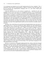
Figure 29.15. The probability
distribution of the state of the
Markov chain for initial condition
x
0
= 17 (example 29.6 (p.372)).
The transition probability matrix of such a chain has more than
one eigenvalue equal to 1.
(b) The chain might have a periodic set, which means that, for some
initial conditions, p
(t)

(x) doesn’t tend to an invariant distribution,
but instead tends to a periodic limit-cycle.
A simple Markov chain with this property is the random walk on the
N-dimensional hypercube. The chain T takes the state from one
corner to a randomly chosen adjacent corner. The unique invariant
distribution of this chain is the uniform distribution over all 2
N
states, but the chain is not ergodic; it is periodic with period two:
if we divide the states into states with odd parity and states with
even parity, we notice that every odd state is surrounded by even
states and vice versa. So if the initial condition at time t = 0 is a
state with even parity, then at time t = 1 – and at all odd times
– the state must have odd parity, and at all even times, the state
will be of even parity.
The transition probability matrix of such a chain has more than
one eigenvalue with magnitude equal to 1. The random walk on
the hypercube, for example, has eigenvalues equal to +1 and −1.
Methods of construction of Markov chains
It is often convenient to construct T by mixing or concatenating simple base
transitions B all of which satisfy
P (x

) =

d
N
x B(x

; x)P(x), (29.43)
for the desired density P (x), i.e., they all have the desired density as an

invariant distribution. These base transitions need not individually be ergodic.
T is a mixture of several base transitions B
b
(x

, x) if we make the transition
by picking one of the base transitions at random, and allowing it to determine
the transition, i.e.,
T (x

, x) =

b
p
b
B
b
(x

, x), (29.44)
where {p
b
} is a probability distribution over the base transitions.
T is a concatenation of two base transitions B
1
(x

, x) and B
2
(x


, x) if we
first make a transition to an intermediate state x

using B
1
, and then make a
transition from state x

to x

using B
2
.
T (x

, x) =

d
N
x

B
2
(x

, x

)B
1

(x

, x). (29.45)
Copyright Cambridge University Press 2003. On-screen viewing permitted. Printing not permitted. />You can buy this book for 30 pounds or $50. See for links.
374 29 — Monte Carlo Methods
Detailed balance
Many useful transition probabilities satisfy the detailed balance property:
T (x
a
; x
b
)P (x
b
) = T(x
b
; x
a
)P (x
a
), for all x
b
and x
a
. (29.46)
This equation says that if we pick (by magic) a state from the target density
P and make a transition under T to another state, it is just as likely that we
will pick x
b
and go from x
b

to x
a
as it is that we will pick x
a
and go from x
a
to x
b
. Markov chains that satisfy detailed balance are also called reversible
Markov chains. The reason why the detailed balance property is of interest
is that detailed balance implies invariance of the distribution P (x) under the
Markov chain T , which is a necessary condition for the key property that we
want from our MCMC simulation – that the probability distribution of the
chain should converge to P (x).
 Exercise 29.7.
[2 ]
Prove that detailed balance implies invariance of the distri-
bution P (x) under the Markov chain T .
Proving that detailed balance holds is often a key step when proving that a
Markov chain Monte Carlo simulation will converge to the desired distribu-
tion. The Metropolis method satisfies detailed balance, for example. Detailed
balance is not an essential condition, however, and we will see later that ir-
reversible Markov chains can be useful in practice, because they may have
different random walk properties.
 Exercise 29.8.
[2 ]
Show that, if we concatenate two base transitions B
1
and B
2

that satisfy detailed balance, it is not necessarily the case that the T
thus defined (29.45) satisfies detailed balance.
Exercise 29.9.
[2 ]
Does Gibbs sampling, with several variables all updated in a
deterministic sequence, satisfy detailed balance?
29.7 Slice sampling
Slice sampling (Neal, 1997a; Neal, 2003) is a Markov chain Monte Carlo
method that has similarities to rejection sampling, Gibbs sampling and the
Metropolis method. It can be applied wherever the Metropolis method can
be applied, that is, to any system for which the target density P
∗
(x) can be
evaluated at any point x; it has the advantage over simple Metropolis methods
that it is more robust to the choice of parameters like step sizes. The sim-
plest version of slice sampling is similar to Gibbs sampling in that it consists of
one-dimensional transitions in the state space; however there is no requirement
that the one-dimensional conditional distributions be easy to sample from, nor
that they have any convexity properties such as are required for adaptive re-
jection sampling. And slice sampling is similar to rejection sampling in that
it is a method that asymptotically draws samples from the volume under the
curve described by P
∗
(x); but there is no requirement for an upper-bounding
function.
I will describe slice sampling by giving a sketch of a one-dimensional sam-
pling algorithm, then giving a pictorial description that includes the details
that make the method valid.
Copyright Cambridge University Press 2003. On-screen viewing permitted. Printing not permitted. />You can buy this book for 30 pounds or $50. See for links.
29.7: Slice sampling 375

The skeleton of slice sampling
Let us assume that we want to draw samples from P (x) ∝ P
∗
(x) where x
is a real number. A one-dimensional slice sampling algorithm is a method
for making transitions from a two-dimensional point (x, u) lying under the
curve P
∗
(x) to another point (x

, u

) lying under the same curve, such that
the probability distribution of (x, u) tends to a uniform distribution over the
area under the curve P
∗
(x), whatever initial point we start from – like the
uniform distribution under the curve P
∗
(x) produced by rejection sampling
(section 29.3).
A single transition (x, u) → (x

, u

) of a one-dimensional slice sampling
algorithm has the following steps, of which steps 3 and 8 will require further
elaboration.
1: evaluate P
∗

(x)
2: draw a vertical coordinate u

∼ Uniform(0, P
∗
(x))
3: create a horizontal interval (x
l
, x
r
) enclosing x
4: loop {
5: draw x

∼ Uniform(x
l
, x
r
)
6: evaluate P
∗
(x

)
7: if P
∗
(x

) > u


break out of loop 4-9
8: else modify the interval (x
l
, x
r
)
9: }
There are several methods for creating the interval (x
l
, x
r
) in step 3, and
several methods for modifying it at step 8. The important point is that the
overall method must satisfy detailed balance, so that the uniform distribution
for (x, u) under the curve P
∗
(x) is invariant.
The ‘stepping out’ method for step 3
In the ‘stepping out’ method for creating an interval (x
l
, x
r
) enclosing x, we
step out in steps of length w until we find endpoints x
l
and x
r
at which P
∗
is

smaller than u. The algorithm is shown in figure 29.16.
3a: draw r ∼ Uniform(0, 1)
3b: x
l
:= x − rw
3c: x
r
:= x + (1 − r)w
3d: while (P
∗
(x
l
) > u

) { x
l
:= x
l
− w }
3e: while (P
∗
(x
r
) > u

) { x
r
:= x
r
+ w }

The ‘shrinking’ method for step 8
Whenever a point x

is drawn such that (x

, u

) lies above the curve P
∗
(x),
we shrink the interval so that one of the end points is x

, and such that the
original point x is still enclosed in the interval.
8a: if (x

> x) { x
r
:= x

}
8b: else { x
l
:= x

}
Properties of slice sampling
Like a standard Metropolis method, slice sampling gets around by a random
walk, but whereas in the Metropolis method, the choice of the step size is
Copyright Cambridge University Press 2003. On-screen viewing permitted. Printing not permitted. />You can buy this book for 30 pounds or $50. See for links.

376 29 — Monte Carlo Methods
1 2
3a,3b,3c 3d,3e
5,6 8
5,6,7
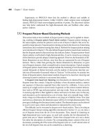
Figure 29.16. Slice sampling. Each
panel is labelled by the steps of
the algorithm that are executed in
it. At step 1, P
∗
(x) is evaluated
at the current point x. At step 2,
a vertical coordinate is selected
giving the point (x, u

) shown by
the box; At steps 3a-c, an
interval of size w containing
(x, u

) is created at random. At
step 3d, P
∗
is evaluated at the left
end of the interval and is found to
be larger than u

, so a step to the
left of size w is made. At step 3e,
P

∗
is evaluated at the right end of
the interval and is found to be
smaller than u

, so no stepping
out to the right is needed. When
step 3d is repeated, P
∗
is found to
be smaller than u

, so the
stepping out halts. At step 5 a
point is drawn from the interval,
shown by a ◦. Step 6 establishes
that this point is above P
∗
and
step 8 shrinks the interval to the
rejected point in such a way that
the original point x is still in the
interval. When step 5 is repeated,
the new coordinate x

(which is to
the right-hand side of the
interval) gives a value of P
∗
greater than u


, so this point x

is
the outcome at step 7.
Copyright Cambridge University Press 2003. On-screen viewing permitted. Printing not permitted. />You can buy this book for 30 pounds or $50. See for links.
29.7: Slice sampling 377
critical to the rate of progress, in slice sampling the step size is self-tuning. If
the initial interval size w is too small by a factor f compared with the width of
the probable region then the stepping-out procedure expands the interval size.
The cost of this stepping-out is only linear in f, whereas in the Metropolis
method the computer-time scales as the square of f if the step size is too
small.
If the chosen value of w is too large by a factor F then the algorithm
spends a time proportional to the logarithm of F shrinking the interval down
to the right size, since the interval typically shrinks by a factor in the ballpark
of 0.6 each time a point is rejected. In contrast, the Metropolis algorithm
responds to a too-large step size by rejecting almost all proposals, so the rate
of progress is exponentially bad in F . There are no rejections in slice sampling.
The probability of staying in exactly the same place is very small.
1 2 3 4 5 6 7 8 9 10 110
1
10
Figure 29.17. P
∗
(x).
 Exercise 29.10.
[2 ]
Investigate the properties of slice sampling applied to the
density shown in figure 29.17. x is a real variable between 0.0 and 11.0.

How long does it take typically for slice sampling to get from an x in
the peak region x ∈ (0, 1) to an x in the tail region x ∈ (1, 11), and vice
versa? Confirm that the probabilities of these transitions do yield an
asymptotic probability density that is correct.
How slice sampling is used in real problems
An N-dimensional density P (x) ∝ P
∗
(x) may be sampled with the help of the
one-dimensional slice sampling method presented above by picking a sequence
of directions y
(1)
, y
(2)
, . and defining x = x
(t)
+ xy
(t)
. The function P
∗
(x)
above is replaced by P
∗
(x) = P
∗
(x
(t)
+ xy
(t)
). The directions may be chosen
in various ways; for example, as in Gibbs sampling, the directions could be the

coordinate axes; alternatively, the directions y
(t)
may be selected at random
in any manner such that the overall procedure satisfies detailed balance.
Computer-friendly slice sampling
The real variables of a probabilistic model will always be represented in a
computer using a finite number of bits. In the following implementation of
slice sampling due to Skilling, the stepping-out, randomization, and shrinking
operations, described above in terms of floating-point operations, are replaced
by binary and integer operations.
We assume that the variable x that is being slice-sampled is represented by
a b-bit integer X taking on one of B = 2
b
values, 0, 1, 2, . . . , B−1, many or all
of which correspond to valid values of x. Using an integer grid eliminates any
errors in detailed balance that might ensue from variable-precision rounding of
floating-point numbers. The mapping from X to x need not be linear; if it is
nonlinear, we assume that the function P
∗
(x) is replaced by an appropriately
transformed function – for example, P
∗∗
(X) ∝ P
∗
(x)|dx/dX|.
We assume the following operators on b-bit integers are available:
X + N arithmetic sum, modulo B, of X and N.
X − N difference, modulo B, of X and N.
X ⊕ N bitwise exclusive-or of X and N .
N := randbits(l) sets N to a random l-bit integer.

A slice-sampling procedure for integers is then as follows:
Copyright Cambridge University Press 2003. On-screen viewing permitted. Printing not permitted. />You can buy this book for 30 pounds or $50. See for links.
378 29 — Monte Carlo Methods
Given: a current point X and a height Y = P
∗
(X) × Uniform(0, 1) ≤ P
∗
(X)
1: U := randbits(b) Define a random translation U of the binary coor-
dinate system.
2: set l to a value l ≤ b Set initial l-bit sampling range.
3: do {
4: N := randbits(l) Define a random move within the current interval of
width 2
l
.
5: X

:= ((X − U) ⊕ N) + U Randomize the lowest l bits of X (in the translated
coordinate system).
6: l := l − 1 If X

is not acceptable, decrease l and try again
7: } until (X

= X) or (P
∗
(X

) ≥ Y ) with a smaller perturbation of X; termination at or

before l = 0 is assured.
The translation U is introduced to avoid permanent sharp edges, where
for example the adjacent binary integers 0111111111 and 1000000000 would
otherwise be permanently in different sectors, making it difficult for X to move
from one to the other.
0
B−1
X
Figure 29.18. The sequence of
intervals from which the new
candidate points are drawn.
The sequence of intervals from which the new candidate points are drawn
is illustrated in figure 29.18. First, a point is drawn from the entire interval,
shown by the top horizontal line. At each subsequent draw, the interval is
halved in such a way as to contain the previous point X.
If preliminary stepping-out from the initial range is required, step 2 above
can be replaced by the following similar procedure:
2a: set l to a value l < b l sets the initial width
2b: do {
2c: N := randbits(l)
2d: X

:= ((X − U) ⊕N ) + U
2e: l := l + 1
2f: } until (l = b) or (P
∗
(X

) < Y )
These shrinking and stepping out methods shrink and expand by a factor

of two per evaluation. A variant is to shrink or expand by more than one bit
each time, setting l := l ± ∆l with ∆l > 1. Taking ∆l at each step from any
pre-assigned distribution (which may include ∆l = 0) allows extra flexibility.
Exercise 29.11.
[4 ]
In the shrinking phase, after an unacceptable X

has been
produced, the choice of ∆l is allowed to depend on the difference between
the slice’s height Y and the value of P
∗
(X

), without spoiling the algo-
rithm’s validity. (Prove this.) It might be a good idea to choose a larger
value of ∆l when Y −P
∗
(X

) is large. Investigate this idea theoretically
or empirically.
A feature of using the integer representation is that, with a suitably ex-
tended number of bits, the single integer X can represent two or more real
parameters – for example, by mapping X to (x
1
, x
2
, x
3
) through a space-filling

curve such as a Peano curve. Thus multi-dimensional slice sampling can be
performed using the same software as for one dimension.
Copyright Cambridge University Press 2003. On-screen viewing permitted. Printing not permitted. />You can buy this book for 30 pounds or $50. See for links.
29.8: Practicalities 379
29.8 Practicalities
Can we predict how long a Markov chain Monte Carlo simulation
will take to equilibrate? By considering the random walks involved in a
Markov chain Monte Carlo simulation we can obtain simple lower bounds on
the time required for convergence. But predicting this time more precisely is a
difficult problem, and most of the theoretical results giving upper bounds on
the convergence time are of little practical use. The exact sampling methods
of Chapter 32 offer a solution to this problem for certain Markov chains.
Can we diagnose or detect convergence in a running simulation?
This is also a difficult problem. There are a few practical tools available, but
none of them is perfect (Cowles and Carlin, 1996).
Can we speed up the convergence time and time between indepen-
dent samples of a Markov chain Monte Carlo method? Here, there is
good news, as described in the next chapter, which describes the Hamiltonian
Monte Carlo method, overrelaxation, and simulated annealing.
29.9 Further practical issues
Can the normalizing constant be evaluated?
If the target density P (x) is given in the form of an unnormalized density
P
∗
(x) with P (x) =
1
Z
P
∗
(x), the value of Z may well be of interest. Monte

Carlo methods do not readily yield an estimate of this quantity, and it is an
area of active research to find ways of evaluating it. Techniques for evaluating
Z include:
1. Importance sampling (reviewed by Neal (1993b)) and annealed impor-
tance sampling (Neal, 1998).
2. ‘Thermodynamic integration’ during simulated annealing, the ‘accep-
tance ratio’ method, and ‘umbrella sampling’ (reviewed by Neal (1993b)).
3. ‘Reversible jump Markov chain Monte Carlo’ (Green, 1995).
One way of dealing with Z, however, may be to find a solution to one’s
task that does not require that Z be evaluated. In Bayesian data modelling
one might be able to avoid the need to evaluate Z – which would be important
for model comparison – by not having more than one model. Instead of using
several models (differing in complexity, for example) and evaluating their rel-
ative posterior probabilities, one can make a single hierarchical model having,
for example, various continuous hyperparameters which play a role similar to
that played by the distinct models (Neal, 1996). In noting the possibility of
not computing Z, I am not endorsing this approach. The normalizing constant
Z is often the single most important number in the problem, and I think every
effort should be devoted to calculating it.
The Metropolis method for big models
Our original description of the Metropolis method involved a joint updating
of all the variables using a proposal density Q(x

; x). For big problems it
may be more efficient to use several proposal distributions Q
(b)
(x

; x), each of
which updates only some of the components of x. Each proposal is individually

accepted or rejected, and the proposal distributions are repeatedly run through
in sequence.
Copyright Cambridge University Press 2003. On-screen viewing permitted. Printing not permitted. />You can buy this book for 30 pounds or $50. See for links.
380 29 — Monte Carlo Methods
 Exercise 29.12.
[2, p.385]
Explain why the rate of movement through the state
space will be greater when B proposals Q
(1)
, . , Q
(B)
are considered
individually in sequence, compared with the case of a single proposal
Q
∗
defined by the concatenation of Q
(1)
, . , Q
(B)
. Assume that each
proposal distribution Q
(b)
(x

; x) has an acceptance rate f < 1/2.
In the Metropolis method, the proposal density Q(x

; x) typically has a
number of parameters that control, for example, its ‘width’. These parameters
are usually set by trial and error with the rule of thumb being to aim for a

rejection frequency of about 0.5. It is not valid to have the width parameters
be dynamically updated during the simulation in a way that depends on the
history of the simulation. Such a modification of the proposal density would
violate the detailed balance condition that guarantees that the Markov chain
has the correct invariant distribution.
Gibbs sampling in big models
Our description of Gibbs sampling involved sampling one parameter at a time,
as described in equations (29.35–29.37). For big problems it may be more
efficient to sample groups of variables jointly, that is to use several proposal
distributions:
x
(t+1)
1
, . , x
(t+1)
a
∼ P (x
1
, . , x
a
|x
(t)
a+1
, . , x
(t)
K
) (29.47)
x
(t+1)
a+1

, . , x
(t+1)
b
∼ P (x
a+1
, . , x
b
|x
(t+1)
1
, . , x
(t+1)
a
, x
(t)
b+1
, . , x
(t)
K
), etc.
How many samples are needed?
At the start of this chapter, we observed that the variance of an estimator
ˆ
Φ
depends only on the number of independent samples R and the value of
σ
2
=

d

N
x P(x)(φ(x) −Φ)
2
. (29.48)
We have now discussed a variety of methods for generating samples from P (x).
How many independent samples R should we aim for?
In many problems, we really only need about twelve independent samples
from P (x). Imagine that x is an unknown vector such as the amount of
corrosion present in each of 10 000 underground pipelines around Cambridge,
and φ(x) is the total cost of repairing those pipelines. The distribution P (x)
describes the probability of a state x given the tests that have been carried out
on some pipelines and the assumptions about the physics of corrosion. The
quantity Φ is the expected cost of the repairs. The quantity σ
2
is the variance
of the cost – σ measures by how much we should expect the actual cost to
differ from the expectation Φ.
Now, how accurately would a manager like to know Φ? I would suggest
there is little point in knowing Φ to a precision finer than about σ/3. After
all, the true cost is likely to differ by ±σ from Φ. If we obtain R = 12
independent samples from P(x), we can estimate Φ to a precision of σ/
√
12 –
which is smaller than σ/3. So twelve samples suffice.
Allocation of resources
Assuming we have decided how many independent samples R are required,
an important question is how one should make use of one’s limited computer
resources to obtain these samples.
Copyright Cambridge University Press 2003. On-screen viewing permitted. Printing not permitted. />You can buy this book for 30 pounds or $50. See for links.
29.10: Summary 381

(1)
(2)
(3)
Figure 29.19. Three possible
Markov chain Monte Carlo
strategies for obtaining twelve
samples in a fixed amount of
computer time. Time is
represented by horizontal lines;
samples by white circles. (1) A
single run consisting of one long
‘burn in’ period followed by a
sampling period. (2) Four
medium-length runs with different
initial conditions and a
medium-length burn in period.
(3) Twelve short runs.
A typical Markov chain Monte Carlo experiment involves an initial pe-
riod in which control parameters of the simulation such as step sizes may be
adjusted. This is followed by a ‘burn in’ period during which we hope the
simulation ‘converges’ to the desired distribution. Finally, as the simulation
continues, we record the state vector occasionally so as to create a list of states
{x
(r)
}
R
r=1
that we hope are roughly independent samples from P (x).
There are several possible strategies (figure 29.19):
1. Make one long run, obtaining all R samples from it.

2. Make a few medium-length runs with different initial conditions, obtain-
ing some samples from each.
3. Make R short runs, each starting from a different random initial condi-
tion, with the only state that is recorded being the final state of each
simulation.
The first strategy has the best chance of attaining ‘convergence’. The last
strategy may have the advantage that the correlations between the recorded
samples are smaller. The middle path is popular with Markov chain Monte
Carlo experts (Gilks et al., 1996) because it avoids the inefficiency of discarding
burn-in iterations in many runs, while still allowing one to detect problems
with lack of convergence that would not be apparent from a single run.
Finally, I should emphasize that there is no need to make the points in
the estimate nearly-independent. Averaging over dependent points is fine – it
won’t lead to any bias in the estimates. For example, when you use strategy
1 or 2, you may, if you wish, include all the points between the first and last
sample in each run. Of course, estimating the accuracy of the estimate is
harder when the points are dependent.
29.10 Summary
• Monte Carlo methods are a powerful tool that allow one to sample from
any probability distribution that can be expressed in the form P (x) =
1
Z
P
∗
(x).
• Monte Carlo methods can answer virtually any query related to P (x) by
putting the query in the form

φ(x)P (x) 
1

R

r
φ(x
(r)
). (29.49)
Copyright Cambridge University Press 2003. On-screen viewing permitted. Printing not permitted. />You can buy this book for 30 pounds or $50. See for links.
382 29 — Monte Carlo Methods
• In high-dimensional problems the only satisfactory methods are those
based on Markov chains, such as the Metropolis method, Gibbs sam-
pling and slice sampling. Gibbs sampling is an attractive method be-
cause it has no adjustable parameters but its use is restricted to cases
where samples can be generated from the conditional distributions. Slice
sampling is attractive because, whilst it has step-length parameters, its
performance is not very sensitive to their values.
• Simple Metropolis algorithms and Gibbs sampling algorithms, although
widely used, perform poorly because they explore the space by a slow
random walk. The next chapter will discuss methods for speeding up
Markov chain Monte Carlo simulations.
• Slice sampling does not avoid random walk behaviour, but it automat-
ically chooses the largest appropriate step size, thus reducing the bad
effects of the random walk compared with, say, a Metropolis method
with a tiny step size.
29.11 Exercises
Exercise 29.13.
[2C, p.386]
A study of importance sampling. We already estab-
lished in section 29.2 that importance sampling is likely to be useless in
high-dimensional problems. This exercise explores a further cautionary
tale, showing that importance sampling can fail even in one dimension,

even with friendly Gaussian distributions.
Imagine that we want to know the expectation of a function φ(x) under
a distribution P (x),
Φ =

dx P (x)φ(x), (29.50)
and that this expectation is estimated by importance sampling with
a distribution Q(x). Alternatively, perhaps we wish to estimate the
normalizing constant Z in P (x) = P
∗
(x)/Z using
Z =

dx P
∗
(x) =

dx Q(x)
P
∗
(x)
Q(x)
=

P
∗
(x)
Q(x)

x∼Q

. (29.51)
Now, let P (x) and Q(x) be Gaussian distributions with mean zero and
standard deviations σ
p
and σ
q
. Each point x drawn from Q will have
an associated weight P
∗
(x)/Q(x). What is the variance of the weights?
[Assume that P
∗
= P , so P is actually normalized, and Z = 1, though
we can pretend that we didn’t know that.] What happens to the variance
of the weights as σ
2
q
→ σ
2
p
/2?
Check your theory by simulating this importance-sampling problem on
a computer.
Exercise 29.14.
[2 ]
Consider the Metropolis algorithm for the one-dimensional
toy problem of section 29.4, sampling from {0, 1, . . . , 20}. Whenever
the current state is one of the end states, the proposal density given in
equation (29.34) will propose with probability 50% a state that will be
rejected.

To reduce this ‘waste’, Fred modifies the software responsible for gen-
erating samples from Q so that when x = 0, the proposal density is
100% on x

= 1, and similarly when x = 20, x

= 19 is always proposed.
Copyright Cambridge University Press 2003. On-screen viewing permitted. Printing not permitted. />You can buy this book for 30 pounds or $50. See for links.
29.11: Exercises 383
Fred sets the software that implements the acceptance rule so that the
software accepts all proposed moves. What probability P

(x) will Fred’s
modified software generate samples from?
What is the correct acceptance rule for Fred’s proposal density, in order
to obtain samples from P (x)?
 Exercise 29.15.
[3C ]
Implement Gibbs sampling for the inference of a single
one-dimensional Gaussian, which we studied using maximum likelihood
in section 22.1. Assign a broad Gaussian prior to µ and a broad gamma
prior (24.2) to the precision parameter β = 1/σ
2
. Each update of µ will
involve a sample from a Gaussian distribution, and each update of σ
requires a sample from a gamma distribution.
Exercise 29.16.
[3C ]
Gibbs sampling for clustering. Implement Gibbs sampling
for the inference of a mixture of K one-dimensional Gaussians, which we

studied using maximum likelihood in section 22.2. Allow the clusters to
have different standard deviations σ
k
. Assign priors to the means and
standard deviations in the same way as the previous exercise. Either fix
the prior probabilities of the classes {π
k
} to be equal or put a uniform
prior over the parameters π and include them in the Gibbs sampling.
Notice the similarity of Gibbs sampling to the soft K-means clustering
algorithm (algorithm 22.2). We can alternately assign the class labels
{k
n
} given the parameters {µ
k
, σ
k
}, then update the parameters given
the class labels. The assignment step involves sampling from the proba-
bility distributions defined by the responsibilities (22.22), and the update
step updates the means and variances using probability distributions
centred on the K-means algorithm’s values (22.23, 22.24).
Do your experiments confirm that Monte Carlo methods bypass the over-
fitting difficulties of maximum likelihood discussed in section 22.4?
A solution to this exercise and the previous one, written in octave, is
available.
2
 Exercise 29.17.
[3C ]
Implement Gibbs sampling for the seven scientists inference

problem, which we encountered in exercise 22.15 (p.309), and which you
may have solved by exact marginalization (exercise 24.3 (p.323)) [it’s
not essential to have done the latter].
 Exercise 29.18.
[2 ]
A Metropolis method is used to explore a distribution P (x)
that is actually a 1000-dimensional spherical Gaussian distribution of
standard deviation 1 in all dimensions. The proposal density Q is a
1000-dimensional spherical Gaussian distribution of standard deviation
. Roughly what is the step size  if the acceptance rate is 0.5? Assuming
this value of ,
(a) roughly how long would the method take to traverse the distribution
and generate a sample independent of the initial condition?
(b) By how much does ln P(x) change in a typical step? By how much
should ln P(x) vary when x is drawn from P(x)?
(c) What happens if, rather than using a Metropolis method that tries
to change all components at once, one instead uses a concatenation
of Metropolis updates changing one component at a time?
2
/>Copyright Cambridge University Press 2003. On-screen viewing permitted. Printing not permitted. />You can buy this book for 30 pounds or $50. See for links.
384 29 — Monte Carlo Methods
 Exercise 29.19.
[2 ]
When discussing the time taken by the Metropolis algo-
rithm to generate independent samples we considered a distribution with
longest spatial length scale L being explored using a proposal distribu-
tion with step size . Another dimension that a MCMC method must
explore is the range of possible values of the log probability ln P
∗
(x).

Assuming that the state x contains a number of independent random
variables proportional to N , when samples are drawn from P (x), the
‘asymptotic equipartition’ principle tell us that the value of −lnP (x) is
likely to be close to the entropy of x, varying either side with a standard
deviation that scales as
√
N. Consider a Metropolis method with a sym-
metrical proposal density, that is, one that satisfies Q(x; x

) = Q(x

; x).
Assuming that accepted jumps either increase ln P
∗
(x) by some amount
or decrease it by a small amount, e.g. ln e = 1 (is this a reasonable
assumption?), discuss how long it must take to generate roughly inde-
pendent samples from P (x). Discuss whether Gibbs sampling has similar
properties.
Exercise 29.20.
[3 ]
Markov chain Monte Carlo methods do not compute parti-
tion functions Z, yet they allow ratios of quantities like Z to be esti-
mated. For example, consider a random-walk Metropolis algorithm in a
state space where the energy is zero in a connected accessible region, and
infinitely large everywhere else; and imagine that the accessible space can
be chopped into two regions connected by one or more corridor states.
The fraction of times spent in each region at equilibrium is proportional
to the volume of the region. How does the Monte Carlo method manage
to do this without measuring the volumes?

Exercise 29.21.
[5 ]
Philosophy.
One curious defect of these Monte Carlo methods – which are widely used
by Bayesian statisticians – is that they are all non-Bayesian (O’Hagan,
1987). They involve computer experiments from which estimators of
quantities of interest are derived. These estimators depend on the pro-
posal distributions that were used to generate the samples and on the
random numbers that happened to come out of our random number
generator. In contrast, an alternative Bayesian approach to the problem
would use the results of our computer experiments to infer the proper-
ties of the target function P (x) and generate predictive distributions for
quantities of interest such as Φ. This approach would give answers that
would depend only on the computed values of P
∗
(x
(r)
) at the points
{x
(r)
}; the answers would not depend on how those points were chosen.
Can you make a Bayesian Monte Carlo method? (See Rasmussen and
Ghahramani (2003) for a practical attempt.)
29.12 Solutions
Solution to exercise 29.1 (p.362). We wish to show that
ˆ
Φ ≡

r
w

r
φ(x
(r)
)

r
w
r
(29.52)
converges to the expectation of Φ under P . We consider the numerator and the
denominator separately. First, the denominator. Consider a single importance
weight
w
r
≡
P
∗
(x
(r)
)
Q
∗
(x
(r)
)
. (29.53)
Copyright Cambridge University Press 2003. On-screen viewing permitted. Printing not permitted. />You can buy this book for 30 pounds or $50. See for links.
29.12: Solutions 385
What is its expectation, averaged under the distribution Q = Q
∗

/Z
Q
of the
point x
(r)
?
w
r
 =

dx Q(x)
P
∗
(x)
Q
∗
(x)
=

dx
1
Z
Q
P
∗
(x) =
Z
P
Z
Q

. (29.54)
So the expectation of the denominator is


r
w
r

= R
Z
P
Z
Q
. (29.55)
As long as the variance of w
r
is finite, the denominator, divided by R, will
converge to Z
P
/Z
Q
as R increases. [In fact, the estimate converges to the
right answer even if this variance is infinite, as long as the expectation is
well-defined.] Similarly, the expectation of one term in the numerator is
w
r
φ(x) =

dx Q(x)
P

∗
(x)
Q
∗
(x)
φ(x) =

dx
1
Z
Q
P
∗
(x)φ(x) =
Z
P
Z
Q
Φ, (29.56)
where Φ is the expectation of φ under P . So the numerator, divided by R,
converges to
Z
P
Z
Q
Φ with increasing R. Thus
ˆ
Φ converges to Φ.
The numerator and the denominator are unbiased estimators of RZ
P

/Z
Q
and RZ
P
/Z
Q
Φ respectively, but their ratio
ˆ
Φ is not necessarily an unbiased
estimator for finite R.
Solution to exercise 29.2 (p.363). When the true density P is multimodal, it is
unwise to use importance sampling with a sampler density fitted to one mode,
because on the rare occasions that a point is produced that lands in one of
the other modes, the weight associated with that point will be enormous. The
estimates will have enormous variance, but this enormous variance may not
be evident to the user if no points in the other mode have been seen.
Solution to exercise 29.5 (p.371). The posterior distribution for the syndrome
decoding problem is a pathological distribution from the point of view of Gibbs
sampling. The factor
[Hn = z] is only 1 on a small fraction of the space of
possible vectors n, namely the 2
K
points that correspond to the valid code-
words. No two codewords are adjacent, so similarly, any single bit flip from
a viable state n will take us to a state with zero probability and so the state
will never move in Gibbs sampling.
A general code has exactly the same problem. The points corresponding
to valid codewords are relatively few in number and they are not adjacent (at
least for any useful code). So Gibbs sampling is no use for syndrome decoding
for two reasons. First, finding any reasonably good hypothesis is difficult, and

as long as the state is not near a valid codeword, Gibbs sampling cannot help
since none of the conditional distributions is defined; and second, once we are
in a valid hypothesis, Gibbs sampling will never take us out of it.
One could attempt to perform Gibbs sampling using the bits of the original
message s as the variables. This approach would not get locked up in the way
just described, but, for a good code, any single bit flip would substantially
alter the reconstructed codeword, so if one had found a state with reasonably
large likelihood, Gibbs sampling would take an impractically large time to
escape from it.
Solution to exercise 29.12 (p.380). Each Metropolis proposal will take the
energy of the state up or down by some amount. The total change in energy
Copyright Cambridge University Press 2003. On-screen viewing permitted. Printing not permitted. />You can buy this book for 30 pounds or $50. See for links.
386 29 — Monte Carlo Methods
when B proposals are concatenated will be the end-point of a random walk
with B steps in it. This walk might have mean zero, or it might have a
tendency to drift upwards (if most moves increase the energy and only a few
decrease it). In general the latter will hold, if the acceptance rate f is small:
the mean change in energy from any one move will be some ∆E > 0 and so
the acceptance probability for the concatenation of B moves will be of order
1/(1 + exp(−B∆E)), which scales roughly as f
B
. The mean-square-distance
moved will be of order f
B
B
2
, where  is the typical step size. In contrast,
the mean-square-distance moved when the moves are considered individually
will be of order fB
2

.
0.2
0.3
0.4
0.5
0.6
0.7
0.8
0.9
1
1.1
0 0.2 0.4 0.6 0.8 1 1.2 1.4 1.6
1000
10000
100000
theory
0
2
4
6
8
10
0 0.2 0.4 0.6 0.8 1 1.2 1.4 1.6
1000
10000
100000
theory
0
0.5
1

1.5
2
2.5
3
3.5
0 0.2 0.4 0.6 0.8 1 1.2 1.4 1.6
Figure 29.20. Importance
sampling in one dimension. For
R = 1000, 10
4
, and 10
5
, the
normalizing constant of a
Gaussian distribution (known in
fact to be 1) was estimated using
importance sampling with a
sampler density of standard
deviation σ
q
(horizontal axis).
The same random number seed
was used for all runs. The three
plots show (a) the estimated
normalizing constant; (b) the
empirical standard deviation of
the R weights; (c) 30 of the
weights.
Solution to exercise 29.13 (p.382). The weights are w = P (x)/Q(x) and x is
drawn from Q. The mean weight is


dx Q(x) [P (x)/Q(x)] =

dx P (x) = 1, (29.57)
assuming the integral converges. The variance is
var(w) =

dx Q(x)

P (x)
Q(x)
− 1

2
(29.58)
=

dx
P (x)
2
Q(x)
− 2P (x) + Q(x) (29.59)
=


dx
Z
Q
Z
2

P
exp

−
x
2
2

2
σ
2
p
−
1
σ
2
q

− 1, (29.60)
where Z
Q
/Z
2
P
= σ
q
/(
√
2πσ
2

p
). The integral in (29.60) is finite only if the
coefficient of x
2
in the exponent is positive, i.e., if
σ
2
q
>
1
2
σ
2
p
. (29.61)
If this condition is satisfied, the variance is
var(w) =
σ
q
√
2πσ
2
p
√
2π

2
σ
2
p

−
1
σ
2
q

−
1
2
− 1 =
σ
2
q
σ
p

2σ
2
q
− σ
2
p

1/2
− 1. (29.62)
As σ
q
approaches the critical value – about 0.7σ
p
– the variance becomes

infinite. Figure 29.20 illustrates these phenomena for σ
p
= 1 with σ
q
varying
from 0.1 to 1.5. The same random number seed was used for all runs, so
the weights and estimates follow smooth curves. Notice that the empirical
standard deviation of the R weights can look quite small and well-behaved
(say, at σ
q
 0.3) when the true standard deviation is nevertheless infinite.
Copyright Cambridge University Press 2003. On-screen viewing permitted. Printing not permitted. />You can buy this book for 30 pounds or $50. See for links.
30
Efficient Monte Carlo Methods
This chapter discusses several methods for reducing random walk behaviour
in Metropolis methods. The aim is to reduce the time required to obtain
effectively independent samples. For brevity, we will say ‘independent samples’
when we mean ‘effectively independent samples’.
30.1 Hamiltonian Monte Carlo
The Hamiltonian Monte Carlo method is a Metropolis method, applicable
to continuous state spaces, that makes use of gradient information to reduce
random walk behaviour. [The Hamiltonian Monte Carlo method was originally
called hybrid Monte Carlo, for historical reasons.]
For many systems whose probability P (x) can be written in the form
P (x) =
e
−E(x)
Z
, (30.1)
not only E(x) but also its gradient with respect to x can be readily evaluated.

It seems wasteful to use a simple random-walk Metropolis method when this
gradient is available – the gradient indicates which direction one should go in
to find states that have higher probability!
Overview of Hamiltonian Monte Carlo
In the Hamiltonian Monte Carlo method, the state space x is augmented by
momentum variables p, and there is an alternation of two types of proposal.
The first proposal randomizes the momentum variable, leaving the state x un-
changed. The second proposal changes both x and p using simulated Hamil-
tonian dynamics as defined by the Hamiltonian
H(x, p) = E(x) + K(p), (30.2)
where K(p) is a ‘kinetic energy’ such as K(p) = p
T
p/2. These two proposals
are used to create (asymptotically) samples from the joint density
P
H
(x, p) =
1
Z
H
exp[−H(x, p)] =
1
Z
H
exp[−E(x)] exp[−K(p)]. (30.3)
This density is separable, so the marginal distribution of x is the desired
distribution exp[−E(x)]/Z. So, simply discarding the momentum variables,
we obtain a sequence of samples {x
(t)
} that asymptotically come from P (x).

387
Copyright Cambridge University Press 2003. On-screen viewing permitted. Printing not permitted. />You can buy this book for 30 pounds or $50. See for links.
388 30 — Efficient Monte Carlo Methods
Algorithm 30.1. Octave source
code for the Hamiltonian Monte
Carlo method.
g = gradE ( x ) ; # set gradient using initial x
E = findE ( x ) ; # set objective function too
for l = 1:L # loop L times
p = randn ( size(x) ) ; # initial momentum is Normal(0,1)
H = p’ * p / 2 + E ; # evaluate H(x,p)
xnew = x ; gnew = g ;
for tau = 1:Tau # make Tau ‘leapfrog’ steps
p = p - epsilon * gnew / 2 ; # make half-step in p
xnew = xnew + epsilon * p ; # make step in x
gnew = gradE ( xnew ) ; # find new gradient
p = p - epsilon * gnew / 2 ; # make half-step in p
endfor
Enew = findE ( xnew ) ; # find new value of H
Hnew = p’ * p / 2 + Enew ;
dH = Hnew - H ; # Decide whether to accept
if ( dH < 0 ) accept = 1 ;
elseif ( rand() < exp(-dH) ) accept = 1 ;
else accept = 0 ;
endif
if ( accept )
g = gnew ; x = xnew ; E = Enew ;
endif
endfor
Hamiltonian Monte Carlo Simple Metropolis

(a)
-1
-0.5
0
0.5
1
-1 -0.5 0 0.5 1
(c)
-1
-0.5
0
0.5
1
-1 -0.5 0 0.5 1
(b)
-1.5
-1
-0.5
0
0.5
1
-1.5 -1 -0.5 0 0.5 1
(d)
-1
-0.5
0
0.5
1
-1 -0.5 0 0.5 1
Figure 30.2. (a,b) Hamiltonian

Monte Carlo used to generate
samples from a bivariate Gaussian
with correlation ρ = 0.998. (c,d)
For comparison, a simple
random-walk Metropolis method,
given equal computer time.
Copyright Cambridge University Press 2003. On-screen viewing permitted. Printing not permitted. />You can buy this book for 30 pounds or $50. See for links.
30.1: Hamiltonian Monte Carlo 389
Details of Hamiltonian Monte Carlo
The first proposal, which can be viewed as a Gibbs sampling update, draws a
new momentum from the Gaussian density exp[−K(p)]/Z
K
. This proposal is
always accepted. During the second, dynamical proposal, the momentum vari-
able determines where the state x goes, and the gradient of E(x) determines
how the momentum p changes, in accordance with the equations
˙
x = p (30.4)
˙
p = −
∂E(x)
∂x
. (30.5)
Because of the persistent motion of x in the direction of the momentum p
during each dynamical proposal, the state of the system tends to move a
distance that goes linearly with the computer time, rather than as the square
root.
The second proposal is accepted in accordance with the Metropolis rule.
If the simulation of the Hamiltonian dynamics is numerically perfect then
the proposals are accepted every time, because the total energy H(x, p) is a

constant of the motion and so a in equation (29.31) is equal to one. If the
simulation is imperfect, because of finite step sizes for example, then some of
the dynamical proposals will be rejected. The rejection rule makes use of the
change in H(x, p), which is zero if the simulation is perfect. The occasional
rejections ensure that, asymptotically, we obtain samples (x
(t)
, p
(t)
) from the
required joint density P
H
(x, p).
The source code in figure 30.1 describes a Hamiltonian Monte Carlo method
that uses the ‘leapfrog’ algorithm to simulate the dynamics on the function
findE(x), whose gradient is found by the function gradE(x). Figure 30.2
shows this algorithm generating samples from a bivariate Gaussian whose en-
ergy function is E(x) =
1
2
x
T
Ax with
A =

250.25 −249.75
−249.75 250.25

, (30.6)
corresponding to a variance–covariance matrix of


1 0.998
0.998 1

. (30.7)
In figure 30.2a, starting from the state marked by the arrow, the solid line
represents two successive trajectories generated by the Hamiltonian dynamics.
The squares show the endpoints of these two trajectories. Each trajectory
consists of Tau = 19 ‘leapfrog’ steps with epsilon = 0.055. These steps are
indicated by the crosses on the trajectory in the magnified inset. After each
trajectory, the momentum is randomized. Here, both trajectories are accepted;
the errors in the Hamiltonian were only +0.016 and −0.06 respectively.
Figure 30.2b shows how a sequence of four trajectories converges from an
initial condition, indicated by the arrow, that is not close to the typical set
of the target distribution. The trajectory parameters Tau and epsilon were
randomized for each trajectory using uniform distributions with means 19 and
0.055 respectively. The first trajectory takes us to a new state, (−1.5, −0.5),
similar in energy to the first state. The second trajectory happens to end in
a state nearer the bottom of the energy landscape. Here, since the potential
energy E is smaller, the kinetic energy K = p
2
/2 is necessarily larger than it
was at the start of the trajectory. When the momentum is randomized before
the third trajectory, its kinetic energy becomes much smaller. After the fourth
Copyright Cambridge University Press 2003. On-screen viewing permitted. Printing not permitted. />You can buy this book for 30 pounds or $50. See for links.
390 30 — Efficient Monte Carlo Methods
Gibbs sampling Overrelaxation
(a)
-1
-0.5
0

0.5
1
-1 -0.5 0 0.5 1
-1
-0.5
0
0.5
1
-1 -0.5 0 0.5 1
(b)
-1
-0.8
-0.6
-0.4
-0.2
0
-1 -0.8-0.6-0.4-0.2 0
(c)
Gibbs sampling
-3
-2
-1
0
1
2
3
0 200 400 600 800 1000 1200 1400 1600 1800 2000
Overrelaxation
-3
-2

-1
0
1
2
3
0 200 400 600 800 1000 1200 1400 1600 1800 2000
Figure 30.3. Overrelaxation
contrasted with Gibbs sampling
for a bivariate Gaussian with
correlation ρ = 0.998. (a) The
state sequence for 40 iterations,
each iteration involving one
update of both variables. The
overrelaxation method had
α = −0.98. (This excessively large
value is chosen to make it easy to
see how the overrelaxation method
reduces random walk behaviour.)
The dotted line shows the contour
x
T
Σ
−1
x = 1. (b) Detail of (a),
showing the two steps making up
each iteration. (c) Time-course of
the variable x
1
during 2000
iterations of the two methods.

The overrelaxation method had
α = −0.89. (After Neal (1995).)
trajectory has been simulated, the state appears to have become typical of the
target density.
Figures 30.2(c) and (d) show a random-walk Metropolis method using a
Gaussian proposal density to sample from the same Gaussian distribution,
starting from the initial conditions of (a) and (b) respectively. In (c) the step
size was adjusted such that the acceptance rate was 58%. The number of
proposals was 38 so the total amount of computer time used was similar to
that in (a). The distance moved is small because of random walk behaviour.
In (d) the random-walk Metropolis method was used and started from the
same initial condition as (b) and given a similar amount of computer time.
30.2 Overrelaxation
The method of overrelaxation is a method for reducing random walk behaviour
in Gibbs sampling. Overrelaxation was originally introduced for systems in
which all the conditional distributions are Gaussian.
An example of a joint distribution that is not Gaussian but whose conditional
distributions are all Gaussian is P (x, y) = exp(−x
2
y
2
− x
2
− y
2
)/Z.
Copyright Cambridge University Press 2003. On-screen viewing permitted. Printing not permitted. />You can buy this book for 30 pounds or $50. See for links.
30.2: Overrelaxation 391
Overrelaxation for Gaussian conditional distributions
In ordinary Gibbs sampling, one draws the new value x

(t+1)
i
of the current
variable x
i
from its conditional distribution, ignoring the old value x
(t)
i
. The
state makes lengthy random walks in cases where the variables are strongly
correlated, as illustrated in the left-hand panel of figure 30.3. This figure uses
a correlated Gaussian distribution as the target density.
In Adler’s (1981) overrelaxation method, one instead samples x
(t+1)
i
from
a Gaussian that is biased to the opposite side of the conditional distribution.
If the conditional distribution of x
i
is Normal(µ, σ
2
) and the current value of
x
i
is x
(t)
i
, then Adler’s method sets x
i
to

x
(t+1)
i
= µ + α(x
(t)
i
− µ) + (1 −α
2
)
1/2
σν, (30.8)
where ν ∼ Normal(0, 1) and α is a parameter between −1 and 1, usually set to
a negative value. (If α is positive, then the method is called under-relaxation.)
Exercise 30.1.
[2 ]
Show that this individual transition leaves invariant the con-
ditional distribution x
i
∼ Normal(µ, σ
2
).
A single iteration of Adler’s overrelaxation, like one of Gibbs sampling, updates
each variable in turn as indicated in equation (30.8). The transition matrix
T (x

; x) defined by a complete update of all variables in some fixed order does
not satisfy detailed balance. Each individual transition for one coordinate
just described does satisfy detailed balance – so the overall chain gives a valid
sampling strategy which converges to the target density P (x) – but when we
form a chain by applying the individual transitions in a fixed sequence, the

overall chain is not reversible. This temporal asymmetry is the key to why
overrelaxation can be beneficial. If, say, two variables are positively correlated,
then they will (on a short timescale) evolve in a directed manner instead of by
random walk, as shown in figure 30.3. This may significantly reduce the time
required to obtain independent samples.
Exercise 30.2.
[3 ]
The transition matrix T (x

; x) defined by a complete update
of all variables in some fixed order does not satisfy detailed balance. If
the updates were in a random order, then T would be symmetric. Inves-
tigate, for the toy two-dimensional Gaussian distribution, the assertion
that the advantages of overrelaxation are lost if the overrelaxed updates
are made in a random order.
Ordered Overrelaxation
The overrelaxation method has been generalized by Neal (1995) whose ordered
overrelaxation method is applicable to any system where Gibbs sampling is
used. In ordered overrelaxation, instead of taking one sample from the condi-
tional distribution P (x
i
|{x
j
}
j=i
), we create K such samples x
(1)
i
, x
(2)

i
, . , x
(K)
i
,
where K might be set to twenty or so. Often, generating K −1 extra samples
adds a negligible computational cost to the initial computations required for
making the first sample. The points {x
(k)
i
} are then sorted numerically, and
the current value of x
i
is inserted into the sorted list, giving a list of K + 1
points. We give them ranks 0, 1, 2, . , K. Let κ be the rank of the current
value of x
i
in the list. We set x

i
to the value that is an equal distance from
the other end of the list, that is, the value with rank K − κ. The role played
by Adler’s α parameter is here played by the parameter K. When K = 1, we
obtain ordinary Gibbs sampling. For practical purposes Neal estimates that
ordered overrelaxation may speed up a simulation by a factor of ten or twenty.
Copyright Cambridge University Press 2003. On-screen viewing permitted. Printing not permitted. />You can buy this book for 30 pounds or $50. See for links.
392 30 — Efficient Monte Carlo Methods
30.3 Simulated annealing
A third technique for speeding convergence is simulated annealing. In simu-
lated annealing, a ‘temperature’ parameter is introduced which, when large,

allows the system to make transitions that would be improbable at temper-
ature 1. The temperature is set to a large value and gradually reduced to
1. This procedure is supposed to reduce the chance that the simulation gets
stuck in an unrepresentative probability island.
We asssume that we wish to sample from a distribution of the form
P (x) =
e
−E(x)
Z
(30.9)
where E(x) can be evaluated. In the simplest simulated annealing method,
we instead sample from the distribution
P
T
(x) =
1
Z(T )
e
−
E(x)
T
(30.10)
and decrease T gradually to 1.
Often the energy function can be separated into two terms,
E(x) = E
0
(x) + E
1
(x), (30.11)
of which the first term is ‘nice’ (for example, a separable function of x) and the

second is ‘nasty’. In these cases, a better simulated annealing method might
make use of the distribution
P

T
(x) =
1
Z

(T )
e
−E
0
(x)−
E
1
(x)
/
T
(30.12)
with T gradually decreasing to 1. In this way, the distribution at high tem-
peratures reverts to a well-behaved distribution defined by E
0
.
Simulated annealing is often used as an optimization method, where the
aim is to find an x that minimizes E(x), in which case the temperature is
decreased to zero rather than to 1.
As a Monte Carlo method, simulated annealing as described above doesn’t
sample exactly from the right distribution, because there is no guarantee that
the probability of falling into one basin of the energy is equal to the total prob-

ability of all the states in that basin. The closely related ‘simulated tempering’
method (Marinari and Parisi, 1992) corrects the biases introduced by the an-
nealing process by making the temperature itself a random variable that is
updated in Metropolis fashion during the simulation. Neal’s (1998) ‘annealed
importance sampling’ method removes the biases introduced by annealing by
computing importance weights for each generated point.
30.4 Skilling’s multi-state leapfrog method
A fourth method for speeding up Monte Carlo simulations, due to John
Skilling, has a similar spirit to overrelaxation, but works in more dimensions.
This method is applicable to sampling from a distribution over a continuous
state space, and the sole requirement is that the energy E(x) should be easy
to evaluate. The gradient is not used. This leapfrog method is not intended to
be used on its own but rather in sequence with other Monte Carlo operators.
Instead of moving just one state vector x around the state space, as was
the case for all the Monte Carlo methods discussed thus far, Skilling’s leapfrog
method simultaneously maintains a set of S state vectors {x
(s)
}, where S
Copyright Cambridge University Press 2003. On-screen viewing permitted. Printing not permitted. />You can buy this book for 30 pounds or $50. See for links.
30.4: Skilling’s multi-state leapfrog method 393
might be six or twelve. The aim is that all S of these vectors will represent
independent samples from the same distribution P (x).
Skilling’s leapfrog makes a proposal for the new state x
(s)

, which is ac-
cepted or rejected in accordance with the Metropolis method, by leapfrogging
x
(s)
x

(t)
x
(s)

the current state x
(s)
over another state vector x
(t)
:
x
(s)

= x
(t)
+ (x
(t)
− x
(s)
) = 2x
(t)
− x
(s)
. (30.13)
All the other state vectors are left where they are, so the acceptance probability
depends only on the change in energy of x
(s)
.
Which vector, t, is the partner for the leapfrog event can be chosen in
various ways. The simplest method is to select the partner at random from
the other vectors. It might be better to choose t by selecting one of the

nearest neighbours x
(s)
– nearest by any chosen distance function – as long
as one then uses an acceptance rule that ensures detailed balance by checking
whether point t is still among the nearest neighbours of the new point, x
(s)

.
Why the leapfrog is a good idea
Imagine that the target density P (x) has strong correlations – for example,
the density might be a needle-like Gaussian with width  and length L, where
L  1. As we have emphasized, motion around such a density by standard
methods proceeds by a slow random walk.
Imagine now that our set of S points is lurking initially in a location that
is probable under the density, but in an inappropriately small ball of size .
Now, under Skilling’s leapfrog method, a typical first move will take the point
a little outside the current ball, perhaps doubling its distance from the centre
of the ball. After all the points have had a chance to move, the ball will have
increased in size; if all the moves are accepted, the ball will be bigger by a
factor of two or so in all dimensions. The rejection of some moves will mean
that the ball containing the points will probably have elongated in the needle’s
long direction by a factor of, say, two. After another cycle through the points,
the ball will have grown in the long direction by another factor of two. So the
typical distance travelled in the long dimension grows exponentially with the
number of iterations.
Now, maybe a factor of two growth per iteration is on the optimistic side;
but even if the ball only grows by a factor of, let’s say, 1.1 per iteration, the
growth is nevertheless exponential. It will only take a number of iterations
proportional to log L/ log(1.1) for the long dimension to be explored.
 Exercise 30.3.

[2, p.398]
Discuss how the effectiveness of Skilling’s method scales
with dimensionality, using a correlated N -dimensional Gaussian distri-
bution as an example. Find an expression for the rejection probability,
assuming the Markov chain is at equilibrium. Also discuss how it scales
with the strength of correlation among the Gaussian variables. [Hint:
Skilling’s method is invariant under affine transformations, so the rejec-
tion probability at equilibrium can be found by looking at the case of a
separable Gaussian.]
This method has some similarity to the ‘adaptive direction sampling’ method
of Gilks et al. (1994) but the leapfrog method is simpler and can be applied
to a greater variety of distributions.
Copyright Cambridge University Press 2003. On-screen viewing permitted. Printing not permitted. />You can buy this book for 30 pounds or $50. See for links.
394 30 — Efficient Monte Carlo Methods
30.5 Monte Carlo algorithms as communication channels
It may be a helpful perspective, when thinking about speeding up Monte Carlo
methods, to think about the information that is being communicated. Two
communications take place when a sample from P (x) is being generated.
First, the selection of a particular x from P (x) necessarily requires that
at least log 1/P (x) random bits be consumed. [Recall the use of inverse arith-
metic coding as a method for generating samples from given distributions
(section 6.3).]
Second, the generation of a sample conveys information about P (x) from
the subroutine that is able to evaluate P
∗
(x) (and from any other subroutines
that have access to properties of P
∗
(x)).
Consider a dumb Metropolis method, for example. In a dumb Metropolis

method, the proposals Q(x

; x) have nothing to do with P (x). Properties
of P (x) are only involved in the algorithm at the acceptance step, when the
ratio P
∗
(x

)/P
∗
(x) is computed. The channel from the true distribution P (x)
to the user who is interested in computing properties of P (x) thus passes
through a bottleneck: all the information about P is conveyed by the string of
acceptances and rejections. If P (x) were replaced by a different distribution
P
2
(x), the only way in which this change would have an influence is that the
string of acceptances and rejections would be changed. I am not aware of much
use being made of this information-theoretic view of Monte Carlo algorithms,
but I think it is an instructive viewpoint: if the aim is to obtain information
about properties of P (x) then presumably it is helpful to identify the channel
through which this information flows, and maximize the rate of information
transfer.
Example 30.4. The information-theoretic viewpoint offers a simple justification
for the widely-adopted rule of thumb, which states that the parameters of
a dumb Metropolis method should be adjusted such that the acceptance
rate is about one half. Let’s call the acceptance history, that is, the
binary string of accept or reject decisions, a. The information learned
about P (x) after the algorithm has run for T steps is less than or equal to
the information content of a, since all information about P is mediated

by a. And the information content of a is upper-bounded by T H
2
(f),
where f is the acceptance rate. This bound on information acquired
about P is maximized by setting f = 1/2.
Another helpful analogy for a dumb Metropolis method is an evolutionary
one. Each proposal generates a progeny x

from the current state x. These two
individuals then compete with each other, and the Metropolis method uses a
noisy survival-of-the-fittest rule. If the progeny x

is fitter than the parent (i.e.,
P
∗
(x

) > P
∗
(x), assuming the Q/Q factor is unity) then the progeny replaces
the parent. The survival rule also allows less-fit progeny to replace the parent,
sometimes. Insights about the rate of evolution can thus be applied to Monte
Carlo methods.
Exercise 30.5.
[3 ]
Let x ∈ {0, 1}
G
and let P (x) be a separable distribution,
P (x) =


g
p(x
g
), (30.14)
with p(0) = p
0
and p(1) = p
1
, for example p
1
= 0.1. Let the proposal
density of a dumb Metropolis algorithm Q involve flipping a fraction m
of the G bits in the state x. Analyze how long it takes for the chain to
Copyright Cambridge University Press 2003. On-screen viewing permitted. Printing not permitted. />You can buy this book for 30 pounds or $50. See for links.
30.6: Multi-state methods 395
converge to the target density as a function of m. Find the optimal m
and deduce how long the Metropolis method must run for.
Compare the result with the results for an evolving population under
natural selection found in Chapter 19.
The insight that the fastest progress that a standard Metropolis method
can make, in information terms, is about one bit per iteration, gives a strong
motivation for speeding up the algorithm. This chapter has already reviewed
several methods for reducing random-walk behaviour. Do these methods also
speed up the rate at which information is acquired?
Exercise 30.6.
[4 ]
Does Gibbs sampling, which is a smart Metropolis method
whose proposal distributions do depend on P (x), allow information about
P (x) to leak out at a rate faster than one bit per iteration? Find toy
examples in which this question can be precisely investigated.

Exercise 30.7.
[4 ]
Hamiltonian Monte Carlo is another smart Metropolis method
in which the proposal distributions depend on P (x). Can Hamiltonian
Monte Carlo extract information about P (x) at a rate faster than one
bit per iteration?
Exercise 30.8.
[5 ]
In importance sampling, the weight w
r
= P
∗
(x
(r)
)/Q
∗
(x
(r)
),
a floating-point number, is computed and retained until the end of the
computation. In contrast, in the dumb Metropolis method, the ratio
a = P
∗
(x

)/P
∗
(x) is reduced to a single bit (‘is a bigger than or smaller
than the random number u?’). Thus in principle importance sampling
preserves more information about P

∗
than does dumb Metropolis. Can
you find a toy example in which this extra information does indeed lead
to faster convergence of importance sampling than Metropolis? Can
you design a Markov chain Monte Carlo algorithm that moves around
adaptively, like a Metropolis method, and that retains more useful in-
formation about the value of P
∗
, like importance sampling?
In Chapter 19 we noticed that an evolving population of N individuals can
make faster evolutionary progress if the individuals engage in sexual reproduc-
tion. This observation motivates looking at Monte Carlo algorithms in which
multiple parameter vectors x are evolved and interact.
30.6 Multi-state methods
In a multi-state method, multiple parameter vectors x are maintained; they
evolve individually under moves such as Metropolis and Gibbs; there are also
interactions among the vectors. The intention is either that eventually all the
vectors x should be samples from P (x) (as illustrated by Skilling’s leapfrog
method), or that information associated with the final vectors x should allow
us to approximate expectations under P (x), as in importance sampling.
Genetic methods
Genetic algorithms are not often described by their proponents as Monte Carlo
algorithms, but I think this is the correct categorization, and an ideal genetic
algorithm would be one that can be proved to be a valid Monte Carlo algorithm
that converges to a specified density.
Copyright Cambridge University Press 2003. On-screen viewing permitted. Printing not permitted. />You can buy this book for 30 pounds or $50. See for links.
396 30 — Efficient Monte Carlo Methods
I’ll use R to denote the number of vectors in the population. We aim to
have P
∗

({x
(r)
}
R
1
) =

P
∗
(x
(r)
). A genetic algorithm involves moves of two or
three types.
First, individual moves in which one state vector is perturbed, x
(r)
→ x
(r)

,
which could be performed using any of the Monte Carlo methods we have
mentioned so far.
Second, we allow crossover moves of the form x, y → x

, y

; in a typical
crossover move, the progeny x

receives half his state vector from one parent,
x, and half from the other, y; the secret of success in a genetic algorithm is

that the parameter x must be encoded in such a way that the crossover of
two independent states x and y, both of which have good fitness P
∗
, should
have a reasonably good chance of producing progeny who are equally fit. This
constraint is a hard one to satisfy in many problems, which is why genetic
algorithms are mainly talked about and hyped up, and rarely used by serious
experts. Having introduced a crossover move x, y → x

, y

, we need to choose
an acceptance rule. One easy way to obtain a valid algorithm is to accept or
reject the crossover proposal using the Metropolis rule with P
∗
({x
(r)
}
R
1
) as
the target density – this involves comparing the fitnesses before and after the
crossover using the ratio
P
∗
(x

)P
∗
(y


)
P
∗
(x)P
∗
(y)
. (30.15)
If the crossover operator is reversible then we have an easy proof that this
procedure satisfies detailed balance and so is a valid component in a chain
converging to P
∗
({x
(r)
}
R
1
).
 Exercise 30.9.
[3 ]
Discuss whether the above two operators, individual varia-
tion and crossover with the Metropolis acceptance rule, will give a more
efficient Monte Carlo method than a standard method with only one
state vector and no crossover.
The reason why the sexual community could acquire information faster than
the asexual community in Chapter 19 was because the crossover operation
produced diversity with standard deviation
√
G, then the Blind Watchmaker
was able to convey lots of information about the fitness function by killing

off the less fit offspring. The above two operators do not offer a speed-up of
√
G compared with standard Monte Carlo methods because there is no killing.
What’s required, in order to obtain a speed-up, is two things: multiplication
and death; and at least one of these must operate selectively. Either we must
kill off the less-fit state vectors, or we must allow the more-fit state vectors to
give rise to more offspring. While it’s easy to sketch these ideas, it is hard to
define a valid method for doing it.
Exercise 30.10.
[5 ]
Design a birth rule and a death rule such that the chain
converges to P
∗
({x
(r)
}
R
1
).
I believe this is still an open research problem.
Particle filters
Particle filters, which are particularly popular in inference problems involving
temporal tracking, are multistate methods that mix the ideas of importance
sampling and Markov chain Monte Carlo. See Isard and Blake (1996), Isard
and Blake (1998), Berzuini et al. (1997), Berzuini and Gilks (2001), Doucet
et al. (2001).
Copyright Cambridge University Press 2003. On-screen viewing permitted. Printing not permitted. />You can buy this book for 30 pounds or $50. See for links.
30.7: Methods that do not necessarily help 397
30.7 Methods that do not necessarily help
It is common practice to use many initial conditions for a particular Markov

chain (figure 29.19). If you are worried about sampling well from a complicated
density P (x), can you ensure the states produced by the simulations are well
distributed about the typical set of P (x) by ensuring that the initial points
are ‘well distributed about the whole state space’?
The answer is, unfortunately, no. In hierarchical Bayesian models, for
example, a large number of parameters {x
n
} may be coupled together via an-
other parameter β (known as a hyperparameter). For example, the quantities
{x
n
} might be independent noise signals, and β might be the inverse-variance
of the noise source. The joint distribution of β and {x
n
} might be
P (β, {x
n
}) = P(β)
N

n=1
P (x
n
|β)
= P(β)
N

n=1
1
Z(β)

e
−βx
2
n
/2
,
where Z(β) =

2π/β and P (β) is a broad distribution describing our igno-
rance about the noise level. For simplicity, let’s leave out all the other variables
– data and such – that might be involved in a realistic problem. Let’s imagine
that we want to sample effectively from P (β, {x
n
}) by Gibbs sampling – alter-
nately sampling β from the conditional distribution P(β |x
n
) then sampling all
the x
n
from their conditional distributions P (x
n
|β). [The resulting marginal
distribution of β should asymptotically be the broad distribution P (β).]
If N is large then the conditional distribution of β given any particular
setting of {x
n
} will be tightly concentrated on a particular most-probable value
of β, with width proportional to 1/
√
N. Progress up and down the β-axis will

therefore take place by a slow random walk with steps of size ∝ 1/
√
N.
So, to the initialization strategy. Can we finesse our slow convergence
problem by using initial conditions located ‘all over the state space’? Sadly,
no. If we distribute the points {x
n
} widely, what we are actually doing is
favouring an initial value of the noise level 1/β that is large. The random
walk of the parameter β will thus tend, after the first drawing of β from
P (β |x
n
), always to start off from one end of the β-axis.
Further reading
The Hamiltonian Monte Carlo method (Duane et al., 1987) is reviewed in Neal
(1993b). This excellent tome also reviews a huge range of other Monte Carlo
methods, including the related topics of simulated annealing and free energy
estimation.
30.8 Further exercises
Exercise 30.11.
[4 ]
An important detail of the Hamiltonian Monte Carlo method
is that the simulation of the Hamiltonian dynamics, while it may be in-
accurate, must be perfectly reversible, in the sense that if the initial con-
dition (x, p) goes to (x

, p

), then the same simulator must take (x


, −p

)
to (x, −p), and the inaccurate dynamics must conserve state-space vol-
ume. [The leapfrog method in algorithm 30.1 satisfies these rules.]
Explain why these rules must be satisfied and create an example illus-
trating the problems that arise if they are not.