Introduction to Optimum Design phần 2 pdf
Bạn đang xem bản rút gọn của tài liệu. Xem và tải ngay bản đầy đủ của tài liệu tại đây (615.83 KB, 76 trang )
Transcribe the problem into the standard design optimization model (also use R
o
£
40.0cm, R
i
£ 40.0cm). Use the following data: P = 14kN; l = 10m; mass density, r
= 7850kg/m
3
; allowable bending stress, s
b
= 165MPa; allowable shear stress, t
a
=
50MPa.
2.24 Design a hollow circular beam shown in Fig. E2-24 for two conditions: when P =
50 (kN), the axial stress s should be less than s
a
, and when P = 0, deflection d due
to self-weight should satisfy d £ 0.001l. The limits for dimensions are t = 0.10 to
1.0cm, R = 2.0 to 20.0cm, and R/t ≥ 20. Formulate the minimum weight design
problem and transcribe it into the standard form. Use the following data: d =
5wl
4
/384EI; w = self weight force/length (N/m); s
a
= 250MPa; modulus of
elasticity, E = 210GPa; mass density, r = 7800kg/m
3
; s = P/A; gravitational
constant, g = 9.80m/s
2
; moment of inertia, I =pR
3
t (m
4
).
t =++
()
P
I
RRRR
ooii
3
22
54 INTRODUCTION TO OPTIMUM DESIGN
PP
2R
t
Beam
A
A
Section A–A
d
l = 3m
FIGURE E2-24 Hollow circular beam.
3 Graphical Optimization
55
Upon completion of this chapter, you will be able to:
•
Graphically solve any optimization problem having two design variables
•
Plot constraints and identify their feasible/infeasible side
•
Identify the feasible region/feasible set for the problem
•
Plot objective function contours through the feasible region
•
Graphically locate the optimum solution for a problem and identify active/inactive
constraints
•
Identify problems that may have multiple, unbounded, or infeasible solutions
Optimization problems having only two design variables can be solved by observing the
way they are graphically represented. All constraint functions are plotted, and a set of
feasible designs (the feasible set) for the problem is identified. Objective function contours
are then drawn and the optimum design is determined by visual inspection. In this chapter,
we illustrate the graphical solution process and introduce several concepts related to optimum
design problems. In the following section, a design optimization problem is formulated and
used to describe the solution process. Some concepts related to design optimization problems
are also described. Several more example problems are solved in later sections to illustrate
the concepts and procedure.
3.1 Graphical Solution Process
3.1.1 Profit Maximization Problem
Step 1: Project/Problem Statement A company manufactures two machines, A and B.
Using available resources, either 28 Aor 14 B machines can be manufactured daily. The sales
department can sell up to 14 A machines or 24 B machines. The shipping facility can handle
no more than 16 machines per day. The company makes a profit of $400 on each A machine
and $600 on each B machine. How many A and B machines should the company manufac-
ture every day to maximize its profit?
Step 2: Data and Information Collection Defined in the project statement.
Step 3: Identification/Definition of Design Variables The following two design variables
are identified in the problem statement:
x
l
= number of A machines manufactured each day
x
2
= number of B machines manufactured each day
Step 4: Identification of a Criterion to Be Optimized The objective is to maximize daily
profit, which can be expressed in terms of design variables as
(a)
Step 5: Identification of Constraints Design constraints are placed on manufacturing
capacity, limitations on the sales personnel, and restrictions on the shipping and handling
facility. The constraint on the shipping and handling facility is quite straightforward,
expressed as
(b)
Constraints on manufacturing and sales facilities are a bit tricky. First, consider the
manufacturing limitation. It is assumed that if the company is manufacturing x
l
A machines
per day, then the remaining resources and equipment can be proportionately utilized to man-
ufacture B number of machines, and vice versa. Therefore, noting that x
l
/28 is the fraction
of resources used to produce A machines and x
2
/14 is the fraction used for B, the constraint
is expressed as
(c)
Similarly, the constraint on sales department resources is given as
(d)
Finally, the design variables must be nonnegative as
(e)
Note that for this problem, the formulation remains valid even when a design variable has
zero value. The problem has two design variables and five inequality constraints. All func-
tions of the problem are linear in variables x
l
and x
2
. Therefore, it is a linear programming
problem.
3.1.2 Step-by-Step Graphical Solution Procedure
Step 1: Coordinate System Set-up The first step in the solution process is to set up an
origin for the x-y coordinate system and scales along the x and y axes. By looking at the con-
straint functions, a coordinate system for the profit maximization problem can be set up using
a range of 0 to 25 along both the x and y axes. In some cases, the scale may need to be
adjusted after the problem has been graphed because the original scale may provide too small
or too large a graph for the problem.
xx
12
0, ≥
xx
12
14 24
1+£
()
limitation on sales department
xx
12
28 14
1+£
()
manufacturing constraint
xx
12
16+£
()
shipping and handling constraint
Px x=+400 600
12
56 INTRODUCTION TO OPTIMUM DESIGN
Step 2: Inequality Constraint Boundary Plot To illustrate the graphing of a constraint, let
us consider the inequality x
1
+ x
2
£ 16, given in Eq. (b). To represent the constraint graphi-
cally, we first need to plot the constraint boundary; i.e., plot the points that satisfy the con-
straint as an equality x
1
+ x
2
= 16. This is a linear function of the variables x
1
and x
2
. To plot
such a function, we need two points that satisfy the equation x
1
+ x
2
= 16. Let these points
be calculated as (16,0) and (0,16). Locating these points on the graph and joining them by
a straight line produces the line F–J, as shown in Fig. 3-1. Line F–J then represents the
boundary of the feasible region for the inequality constraint x
1
+ x
2
£ 16. Points on one side
of this line will violate the constraint, while those on the other side will satisfy it.
Step 3: Identification of Feasible Region for an Inequality The next task is to determine
which side of constraint boundary F–J is feasible for the constraint x
1
+ x
2
£ 16. To accom-
plish this task, we select a point on either side of F–J at which to evaluate the constraint. For
example, at point (0,0), the left side of the constraint x
1
+ x
2
£ 16 has a value of 0. Because
the value is less than 16, the constraint is satisfied and the region below F–J is feasible. We
can test the constraint at another point on the opposite side of F–J, say at point (10,10). At
this point the constraint is violated because the left side of the constraint function is 20, which
is larger than 16. Therefore, the region above F–J is infeasible with respect to the constraint
x
1
+ x
2
£ 16, as shown in Fig. 3-2. The infeasible region is “shaded-out” or “hatched-out,” a
convention that is used throughout this text. Note that if this was an equality constraint x
1
+
x
2
= 16, then the feasible region for the constraint would only be the points on line F–J.
Although there is an infinite number of points on F–J, the feasible region for the equality
constraint is much smaller than that for the same constraint written as an inequality.
Step 4: Identification of Feasible Region By following the procedure described in Step
3, all constraints are plotted on the graph and the feasible region for each constraint is
identified. Note that the constraints x
1
, x
2
≥ 0 restrict the feasible region to the first quadrant
Graphical Optimization 57
0 5 10 15 20 25
0
5
10
15
20
25
x
1
x
2
Profit Maximization Problem
F
(0,16)
J
(16,0)
x
1
+ x
2
= 16
FIGURE 3-1 Constraint boundary for the inequality x
1
+ x
2
£ 16.
of the coordinate system. The intersection of feasible regions for all constraints provides the
feasible region for the profit maximization problem, indicated as ABCDE in Fig. 3-3. Any
point in this region or on its boundary provides a feasible solution to the problem.
Step 5: Plotting Objective Function Contours The next task is to plot the objective func-
tion on the graph and locate its optimum points. For the present problem, the objective is to
maximize the profit, P = 400x
1
+ 600x
2
, which involves three variables: P, x
1
, and x
2
. The
function needs to be represented on the graph so that the value of P can be compared for dif-
ferent feasible designs and the best design can be located. However, because there is an infi-
nite number of feasible points, it is not possible to evaluate the objective function at every
point. One way of overcoming this impasse is to plot the contours of the objective function.
A contour is a curve on the graph that connects all points having the same objective func-
tion value. A collection of points on a contour is also called the level set. If the objective
function is to be minimized, the contours are also called iso-cost curves. To plot a contour
through the feasible region, we need to assign it a value. To obtain this value, consider a
point in the feasible region and evaluate the profit function there. For example, at point (6,4),
P is P = 6 ¥ 400 + 4 ¥ 600 = 4800. To plot the P = 4800 contour, we plot the function 400x
1
+ 600x
2
= 4800. This contour is shown in Fig. 3-4.
Step 6: Identification of Optimum Solution To locate an optimum point for the objective
function, we need at least two contours that pass through the feasible region. We can then
observe trends for the values of the objective function at different feasible points to locate
the best solution point. Contours for P = 2400, 4800, and 7200 are plotted in Fig. 3-5. We
now observe the following trend: as the contours move up toward point D, feasible designs
can be found with larger values for P. It is clear from observation that point D has the largest
value for P in the feasible region. We now simply read the coordinates of point D (4,12) to
obtain the optimum design, having a maximum value for the profit function as P = 8800.
58 INTRODUCTION TO OPTIMUM DESIGN
0 5 10 15 20 25
0
5
10
15
20
F
J
25
x
1
x
2
Profit Maximization Problem
(10,10)
(0,0)
x
1
+ x
2
= 16
Infeasible
x
1
+ x
2
> 16
Feasible
x
1
+ x
2
< 16
FIGURE 3-2 Feasible/infeasible side for the inequality x
1
+ x
2
£ 16.
Graphical Optimization 59
0 5 10 15 20 25
0
5
10
15
20
25
x
1
x
2
Profit Maximization Problem
g
1
g
2
g
3
g
5
g
4
Feasible
E
D
C
B
A
FIGURE 3-3 Feasible region for the profit maximization problem.
0 5 10 15 20 25
0
5
10
15
20
25
x
1
x
2
Profit Maximization Problem
P = 4800
FIGURE 3-4 Plot of P = 4800 objective function contour for the profit maximization problem.
Thus, the best strategy for the company is to manufacture 4 A and 12 B machines to maxi-
mize its daily profit. The inequality constraints in Eqs. (b) and (c) are active at the optimum;
i.e., they are satisfied at equality. These represent limitations on shipping and handling facil-
ities, and manufacturing. The company can think about relaxing these constraints to improve
its profit. All other inequalities are strictly satisfied, and therefore, inactive.
Note that in this example the design variables must have integer values. Fortunately, the
optimum solution has integer values for the variables. If this were not the case, we would
have used the procedure suggested in Section 2.11.4 or in Chapter 15 to solve this problem.
Note also that for this example all functions are linear in design variables. Therefore, all
curves in Figs. 3-1 through 3-5 are straight lines. In general, the functions of a design problem
may not be linear, in which case curves must be plotted to identify the feasible region, and
contours or iso-cost curves must be drawn to identify the optimum design. To plot a non-
linear function, a table of numerical values for x
l
and x
2
must be generated for the function.
These points must be then plotted on a graph and connected by a smooth curve.
3.2 Use of Mathematica for Graphical Optimization
It turns out that good programs, such as Mathematica, are available to implement the step-
by-step procedure of the previous section and obtain a graphical solution for the problem on
the computer screen. Mathematica is an interactive software package with many capabilities;
however, we shall explain its use to solve a two-variable optimization problem by plotting
all functions on the computer screen. Although other commands for plotting functions are
available, the most convenient one for working with inequality constraints and objective func-
tion contours is the ContourPlot command. As with most Mathematica commands, this
command is followed by what we call subcommands as “arguments” that define the nature
60 INTRODUCTION TO OPTIMUM DESIGN
0 5 10 15 20 25
0
5
10
15
20
25
x
2
x
1
Profit Maximization Problem
g1
g2
g3
g5
g4
G
C
D
A
B J H
E
F
P = 8800
P = 2400
FIGURE 3-5 Graphical solution for the profit maximization problem. Optimum point D = (4,
12). Maximum profit, P = 8800.
of the plot. All Mathematica commands are case sensitive so it is important to pay attention
to which letters are capitalized.
Mathematica input is organized into what is called a “notebook.” A notebook is divided
into cells with each cell containing input that can be executed independently. For explaining
the graphical optimization capability of Mathematica5, we shall use the profit maximization
problem of the previous section. Note that the commands used here may change in future
releases of the program. We start by entering into the notebook the problem functions as
P=400*x1+600*x2;
g1=x1+x2-16; (*shipping and handling constraint*)
g2=x1/28+x2/14-1; (*manufacturing constraint*)
g3=x1/14+x2/24-1; (*limitation on sales department*)
g4=-x1;
g5=-x2;
This input illustrates some basic features concerning Mathematica format. Note that the
ENTER key acts simply as a carriage return, taking the blinking cursor to the next line. Press-
ing SHIFT and ENTER actually inputs the typed information into Mathematica. When no
immediate output from Mathematica is desired, the input line must end with a semicolon (;).
If the semicolon is omitted, Mathematica will simplify the input and display it on the screen
or execute an arithmetic expression and display the result. Comments are bracketed as
(*Comment*). Note also that all the constraints are assumed to be in the standard “£” form.
This helps in identifying the infeasible region for constraints on the screen using the Con-
tourPlot command.
3.2.1 Plotting Functions
The Mathematica command used to plot the contour of a function, say g1 = 0, is entered as
Plotg1=ContourPlot[g1,{x1,0,25},{x2,0,25}, ContourShadingÆFalse, ContoursÆ{0},
ContourStyleÆ{{Thickness[.01]}}, AxesÆTrue, AxesLabelÆ{“x1”,”x2”},
PlotLabelÆ“Profit Maximization Problem”, EpilogÆ{Disk[{0,16},{.4,.4}],
Text[“(0,16)”,{2,16}], Disk[{16,0},{.4,.4}], Text[“(16,0)”,{17,1.5}],
Text[“F”,{0,17}], Text[“J”,{17,0}], Text[“x1+x2=16”,{13,9}],
Arrow[{13,8.3},{10,6}]}, DefaultFontÆ{“Times”,12}, ImageSizeÆ72 5];
Plotg1 is simply an arbitrary name referring to the data points for the function g1 deter-
mined by the ContourPlot command; it is used in future commands to refer to this particu-
lar plot. This ContourPlot command plots a contour defined by the equation g1 = 0 as in Fig.
3-1. Arguments of the ContourPlot command containing various subcommands are explained
as follows (note that the arguments are separated by commas and are enclosed in square
brackets []):
g1: function to be plotted.
{x1, 0, 25}, {x2, 0, 25}: ranges for the variables x1 and x2; 0 to 25.
ContourShading Æ False: indicates that shading will not be used to plot contours,
whereas ContourShading Æ True would indicate that shading will be used (note that
most subcommands are followed by an arrow “Æ” or “->” and a set of parameters
enclosed in braces {}).
Contours Æ {0}: contour values for g1, one contour is requested having 0 value.
ContourStyle Æ {{Thickness[.01]}}: defines characteristics of the contour such as
thickness and color. Here, the thickness of the contour is specified as “.01”. It is
Graphical Optimization 61
given as a fraction of the total width of the graph and needs to be determined by trial
and error.
Axes Æ True: indicates whether axes should be drawn at the origin; in the present case,
where the origin (0, 0) is located at the bottom left corner of the graph, the Axes
subcommand is irrelevant except that it allows for the use of the AxesLabel
command.
AxesLabel Æ {“x1”,“x2”}: allows one to indicate labels for each axis.
PlotLabel Æ “Profit Maximization Problem”: puts a label at the top of the graph.
Epilog Æ {. . .}: allows insertion of additional graphics primitives and text in the figure
on the screen; Disk [{0,16}, {.4,.4}] allows insertion of a dot at the location (0,16)
of radius .4 in both directions; Text [“(0,16)”, (2,16)] allows “(0,16)” to be placed at
the location (2,16).
ImageSize Æ 72 5: indicates that the width of the plot should be 5 inches; the size of
the plot also can be adjusted by selecting the image in Mathematica and dragging
one of the black square control points; the images in Mathematica can be copied and
pasted to a word processor file.
DefaultFont Æ {“Times”,12}: specifies the preferred font and size for the text.
3.2.2 Identification and Hatching of Infeasible Region for an Inequality
Figure 3-2 is created using a slightly modified ContourPlot command used earlier for
Fig. 3-1:
Plotg1=ContourPlot[g1,{x1,0,25},{x2,0,25}, ContourShadingÆFalse,ContoursÆ{0,.65},
ContourStyleÆ{{Thickness[.01]},{GrayLevel[.8],Thickness[.025]}}, AxesÆTrue,
AxesLabelÆ{“x1”,”x2”}, PlotLabelÆ“Profit Maximization Problem”,
EpilogÆ{Disk[{10,10},{.4,.4}], Text[“(10,10)”,{11,9}], Disk[{0,0},{.4,.4}],
Text[“(0,0)”,{2,.5}], Text[“x1+x2=16”,{18,7}], Arrow[{18,6.3},{12,4}],
Text[“Infeasible”,{17,17}], Text[“x1+x2>16”,{17,15.5}], Text[“Feasible”,{5,6}],
Text[“x1+x2<16”,{5,4.5}]}, DefaultFontÆ{“Times”,12}, ImageSizeÆ72 5];
Here, two contour lines are specified, the second one having a small positive value. This
is indicated by the command: Contours Æ {0, .65}. The constraint boundary is represented
by the contour g1 = 0. The contour g1 = 0.65 will pass through the infeasible region, where
the positive number 0.65 is determined by trial and error. To shade the infeasible region, the
characteristics of the contour are changed. Each set of brackets {} with the ContourStyle
subcommand corresponds to a specific contour. In this case, {Thickness[.01]} provides
characteristics for the first contour g1 = 0, and {GrayLevel[.8],Thickness[0.025]} provides
characteristics for the second contour g1 = 0.65. GrayLevel specifies a color for the contour
line. A gray level of 0 yields a black line, whereas a gray level of 1 yields a white line. Thus,
this ContourPlot command essentially draws one thin, black line and one thick, gray line.
This way the infeasible side of an inequality is shaded out.
3.2.3 Identification of Feasible Region
By using the foregoing procedure, all constraint functions for the problem are plotted and
their feasible sides are identified. The plot functions for the five constraints g1 to g5 are
named Plotg1, Plotg2, Plotg3, Plotg4, Plotg5. All these functions are quite similar to the one
that was created using the ContourPlot command explained earlier. As an example, Plotg4
function is given as
Plotg4=ContourPlot[g4,{x1,-1,25},{x2,-1,25}, ContourShadingÆFalse,
ContoursÆ{0,.35}, ContourStyleÆ{{Thickness[.01]}, {GrayLevel[.8],Thickness[.02]}},
DisplayFunctionÆIdentity];
62 INTRODUCTION TO OPTIMUM DESIGN
The DisplayFunction Æ Identity subcommand is added to the ContourPlot command to
suppress display of output from each Plotgi function; without that Mathematica executes each
Plotgi function and displays the results. Next, with the following Show command, the five
plots are combined to display the complete feasible set in Fig. 3-3:
Show[{Plotg1,Plotg2,Plotg3,Plotg4,Plotg5}, AxesÆTrue,AxesLabelÆ{“x1”,”x2”},
PlotLabelÆ“Profit Maximization Problem”, DefaultFontÆ{“Times”,12}, EpilogÆ
{Text[“g1”,{2.5,16.2}], Text[“g2”,{24,4}], Text[“g3”,{2,24}], Text[“g5”,{21,1}],
Text[“g4”,{1,10}], Text[“Feasible”,{5,6}]}, DefaultFontÆ{“Times”,12}, ImageSizeÆ72
5,DisplayFunction Æ $DisplayFunction];
The Text subcommands are included to add text to the graph at various locations. The
DisplayFunction Æ $DisplayFunction subcommand is added to display the final graph;
without that it is not displayed.
3.2.4 Plotting of Objective Function Contours
The next task is to plot the objective function contours and locate its optimum point. The
objective function contours of values 2400, 4800, 7200, 8800, shown in Fig. 3-4 are drawn
by using the ContourPlot command as follows:
PlotP=ContourPlot[P,{x1,0,25},{x2,0,25}, ContourShadingÆFalse, ContoursÆ{4800},
ContourStyleÆ{{Dashing[{.03,.04}], Thickness[.007]}}, AxesÆTrue,
AxesLabelÆ{“x1”,”x2”}, PlotLabelÆ“Profit Maximization Problem”,
DefaultFontÆ{“Times”,12}, EpilogÆ{Disk[{6,4},{.4,.4}], Text[“P= 4800”,{9.75,4}]},
ImageSizeÆ72 5];
The ContourStyle subcommand provides four sets of characteristics, one for each
contour. Dashing[{a,b}] yields a dashed line with “a” as the length of each dash and “b” as
the space between dashes. These parameters represent a fraction of the total width of the
graph.
3.2.5 Identification of Optimum Solution
The Show command used to plot the feasible region for the problem in Fig. 3-3 can be
extended to plot the profit function contours as well. Figure 3-5 contains the graphical
representation for the problem obtained using the following Show command:
Show[{Plotg1,Plotg2,Plotg3,Plotg4,Plotg5, PlotP}, AxesÆTrue, AxesLabelÆ{“x1”,”x2”},
PlotLabel Æ “Profit Maximization Problem”, DefaultFontÆ{“Times”,12},
EpilogÆ{Text[“g1”,{2.5,16.2}], Text[“g2”,{24,4}], Text[“g3”,{3,23}], Text[“g5”,{23,1}],
Text[“g4”,{1,10}], Text[“P= 2400”,{3.5,2}], Text[“P= 8800”,{17,3.5}], Text[“G”,{1,24.5}],
Text[“C”,{10.5,4}], Text[“D”,{3.5,11}], Text[“A”,{1,1}], Text[“B”,{14,-1}],Text[“J”,{16,-1}],
Text[“H”,{25,-1}], Text[“E”,{-1,14}], Text[“F”,{-1,16}]}, DefaultFontÆ{“Times”,12},
ImageSizeÆ72 5, DisplayFunction Æ$DisplayFunction];
Additional Text subcommands have been added to label different objective function
contours and different points. The final graph is used to obtain the graphical solution.
The Disk subcommand can be added to the Epilog command to put a dot at the optimum
point.
Graphical Optimization 63
3.3 Use of MATLAB for Graphical Optimization
MATLAB is another software package that has many capabilities to solve engineering prob-
lems. For example, it can be used to plot problem functions and to solve graphically a two-vari-
able optimization problem. In this section, we shall explain use of the program for this purpose;
other uses of the program for solving optimization problems are explained in Chapter 12.
There are two modes of input with MATLAB. One may enter commands interactively, one at
a time, and results are displayed immediately after each command. Alternatively, one may
create an input file, called an M-file, that is executed in batch mode. The M-file can be created
using the text editor in MATLAB. To access this editor, select “File”, “New”, and “M-file”.
When saved, this file will have a suffix of “.m.” To submit or run the file, after starting
MATLAB, simply type the name of the file you wish to run, without the suffix “.m” (the
current directory must be the directory where the file is located). In this section, we shall solve
the profit maximization problem of previous sections using MATLAB6.5. It is important to
note with future releases, the commands discussed below may change.
3.3.1 Plotting of Function Contours
For contour plots, the fist command in the input file is entered as follows:
[x1,x2]=meshgrid(-1.0:0.5:25.0, -1.0:0.5:25.0);
This command creates a grid or array of points where all functions to be plotted are evaluated.
The command indicates that x1 and x2 will start at -1.0 and increase in increments of 0.5 up to
25.0. These variables now represent two-dimensional arrays and require special attention in
operations with them. “*” and “/” indicate scalar multiplication and division respectively,
whereas “.*” and “./” indicate element-by-element multiplication and division. “.Ÿ” is used to
apply an exponent to each element of a vector or a matrix. The semicolon “;” after a command
prevents MATLAB from displaying the numerical results immediately, i.e., all of the values for
x1 and x2. This use of a semicolon is a MATLAB convention for most commands. The
“contour” command is used for plotting all problem functions on the screen. The “.m file” for
the profit maximization problem with explanatory comments is prepared and displayed in Table
3-1. Note that the comments in the “.m file” are preceded by the percent sign, %. The comments
are ignored during MATLAB execution. Also note that matrix division and multiplication capa-
bilities are not used in the present example as the variables in the problem functions are only
multiplied or divided by a scalar rather than another variable. If, for instance, a term such as
x
1
x
2
was present, then the element-by-element operation x1.*x2 would be necessary.
The procedure used to identify the infeasible side of an inequality is the same as explained
in the previous section. Two contours are plotted for the inequality; one of value 0 and the
other of small positive value. The second contour will pass through the infeasible region for
the problem. The thickness of the infeasible contour is changed to indicate the infeasible side
of the inequality using the graph editing capability that is explained in the next section. This
way all the constraint functions are plotted and the feasible region for the problem is identi-
fied. By observing the trend of the objective function contours, we can identify the optimum
point for the problem.
3.3.2 Editing of Graph
Once the graph has been created using the previous commands, it is possible to edit it before
printing it or copying it to a text editor. In particular, one may need to modify the appear-
ance of the infeasible contours of the constraints and edit text in the graph. To do this, first
select “Current Object Properties . . .” under the “Edit” tab on the graph window. Then,
double click any item in the graph to edit its properties. For instance, one may increase the
thickness of the infeasible contours to hatch out the infeasible region. In addition, text may
64 INTRODUCTION TO OPTIMUM DESIGN
Graphical Optimization 65
TABLE 3-1 MATLAB File for Profit Maximization Problem
%Create a grid from -1 to 25 with an increment of 0.5 for the variables x1 and x2
[x1,x2]=meshgrid(-1:0.5:25.0,-1:0.5:25.0);
%Enter functions for the profit maximization problem
f=400*x1+600*x2;
g1=x1+x2-16;
g2=x1/28+x2/14-1;
g3=x1/14+x2/24-1;
g4=-x1;
g5=-x2;
%Initialization statements; these need not end with a semicolon
cla reset
axis auto
%Minimum and maximum values for axes are
determined automatically
%Limits for x- and y-axes may also be specified with
the command
%axis ([xmin xmax ymin ymax])
xlabel(‘x1’),ylabel(‘x2’)
%Specifies labels for x- and y-axes
title (‘Profit Maximization Problem’)
%Displays a title for the problem
hold on
%retains the current plot and axes properties for all
subsequent plots
%Use the “contour” command to plot constraint and cost functions
cv1=[0 .5];
%Specifies two contour values
const1=contour(x1,x2,g1,cv1,‘k’);
%Plots two specified contours of g1; k = black color
clabel(const1)
%Automatically puts the contour value on the graph
text(1,16,‘g1’)
%Writes g1 at the location (1, 16)
cv2=[0 .03];
const2=contour(x1,x2,g2,cv2,‘k’);
clabel(const2)
text(23,3,‘g2’)
const3=contour(x1,x2,g3,cv2,‘k’);
clabel(const3)
text(1,23,‘g3’)
cv3=[0 .5];
const4=contour(x1,x2,g4,cv3,‘k’);
clabel(const4)
text(.25,20,‘g4’)
const5=contour(x1,x2,g5,cv3,‘k’);
clabel(const5)
text(19,.5,‘g5’)
text(1.5,7,’Feasible Region’)
fv=[2400, 4800, 7200, 8800];
%Defines 4 contours for the profit function
fs=contour(x1,x2,f,fv,‘k–’);
%‘k–’ specifies black dashed lines for profit function
contours
clabel(fs)
hold off
%Indicates end of this plotting sequence
%Subsequent plots will appear in separate windows
be added, deleted, or moved as desired. Note that if MATLAB is rerun, any changes made
directly to the graph are lost. For this reason, it is a good idea to save the graph as a “.fig”
file, which then may be recalled with MATLAB. There are two ways for transferring the
graph to another document. First, select “Copy Figure” under the “Edit” tab. The figure then
can be pasted as a bitmap into another document. Alternatively, one may select “Export ”
under the “File” tab. The figure is exported as the specified file type and then can be inserted
into another document through the “Insert” command. The final graph with MATLAB for
the profit maximization problem is shown in Fig. 3-6.
3.4 Design Problem with Multiple Solutions
A situation can arise in which a constraint is parallel to the cost function. If the constraint is
active at the optimum, then there are multiple solutions to the problem. To illustrate this
situation, consider the following design problem: minimize f(x) =-x
1
- 0.5x
2
subject to four
inequality constraints
In this problem, the second constraint is parallel to the cost function. Therefore, there is
a possibility of multiple optimum designs. Figure 3-7 provides a graphical solution to the
problem. It can be seen that any point on the line B–C gives an optimum design. Thus the
problem has infinite optimum solutions.
3.5 Problem with Unbounded Solution
Some design problems may not have a bounded solution. This situation can arise if we forget
a constraint or incorrectly formulate the problem. To illustrate such a situation, consider the
23122 8 0 0
12 12 1 2
xx xx x x+ £ +£ -£-£,,,
66 INTRODUCTION TO OPTIMUM DESIGN
-5 0 5 10 15 20 25
-5
0
5
10
15
20
25
x
1
x
2
Profit Maximization Problem
g1
g2
g3
g4
g5
2400
4800
7200
8800
A
B
J
H
C
D
E
F
G
Optimum
point
Feasible Region
FIGURE 3-6 Graphical representation for the profit maximization problem with MATLAB.
following design problem: minimize f(x) =-x
1
+ 2x
2
subject to four inequality
constraints
The feasible set for the problem is shown in Fig. 3-8. Several cost function contours are
shown. It can be seen that the feasible set is unbounded. Therefore, there is no finite optimum
solution. We must re-examine the way the problem was formulated to correct the situation.
It can be seen in Fig. 3-8 that the problem is under-constrained.
3.6 Infeasible Problem
If we are not careful in formulating a design problem, it may not have a solution, which
happens when there are conflicting requirements or inconsistent constraint equations. There
may also be no solution when we put too many constraints on the system, i.e., the constraints
are so restrictive that no feasible solution is possible. These are called infeasible problems.
To illustrate such a situation, consider the following problem: minimize f(x) = x
1
+ 2x
2
subject
to six inequality constraints
Constraints for the problem are plotted in Fig. 3-9. It can be seen that there is no region
within the design space that satisfies all constraints. Thus, the problem is infeasible. Basi-
32 62312 5 0
1 2 1 2 12 12
x x x x xx xx+£ +≥ £ ≥,,,,,
-+£ -+ £ -£-£2023600
12 1 2 1 2
xx x x x x,,,
Graphical Optimization 67
10
2x
1
+ x
2
= 8
2x
1
+ 3x
2
= 12
8
6
4
2
x
2
x
1
Optimum solution line B–C
B
A
D
2468
f = -4
f = -3
f = -2
f = -1
C
FIGURE 3-7 Example problem with multiple solutions.
68 INTRODUCTION TO OPTIMUM DESIGN
10
2x
1
- x
2
= 0
-
2x
1
+ 3x
2
= 6
8
6
4
2
x
2
x
1
B
C
A
D
24 68
f = 4
f = -4
f = 0
FIGURE 3-8 Example problem with unbounded solution.
2x
1
+ 3x
2
= 12
3x
1
+ 2x
2
= 6
x
2
x
1
x
1
= 5
x
2
= 5
6
4
2
246
0
F
G
E
A
B
C
D
FIGURE 3-9 Example of infeasible design optimization problem.
cally, the first two constraints impose conflicting requirements on the design problem. The
first requires the feasible design to be below the line A–G, whereas the second requires it to
be above the line C–F. Since the two lines do not intersect in the first quadrant, there is no
feasible region for the problem.
3.7 Graphical Solution for Minimum Weight Tubular Column
The design problem formulated in Section 2.7 will now be solved using the graphical method,
with the following specifications: P = 10MN, E = 207GPa, r = 7833kg/m
3
, l = 5.0m, and
s
a
= 248MPa. Using this data, Formulation 1 for the problem is defined as: find mean radius
R (m) and thickness t (m) to minimize the mass function:
(a)
subject to the four inequality constraints
(b)
(c)
(d)
(e)
Note that the explicit bound constraints are simply replaced by the nonnegativity
constraints g
3
and g
4
. The constraints for the problem are plotted in Fig. 3-10 and the
feasible region is indicated. Cost function contours for f = 1000, 1500, 1579kg are also
shown. Note that in this example the cost function contours run parallel to the stress con-
straint g
1
. Since g
1
is active at the optimum, the problem has an infinite number of optimum
designs, i.e., the entire curve A–B in Fig. 3-10. We can read the coordinates of any point on
the curve A–B as an optimum solution. In particular, point A, where constraints g
1
and g
2
intersect, is also an optimum point where R* = 0.1575m and t* = 0.0405m. Note that the
superscript * on a variable indicates its optimum value, a notation that will be used through-
out this text.
Note also that this problem has nonlinear functions. To plot them, we generate tables
of data points t versus R and connect them using smooth curves on the graph. For example,
to plot the constraint boundary for g
2
(R
3
t = 1.558 ¥ 10
-4
), we select values for t as
0.015, 0.03, 0.06, 0.075, 0.09, and calculate the values for R from g
2
= 0 as 0.218, 0.173,
0.1374, 0.1275, and 0.12. This procedure can be used to plot any nonlinear function of two
variables. Figure 3-10 was generated using MATLAB with manual hatching of the infeasi-
ble region.
3.8 Graphical Solution for a Beam Design Problem
Step 1: Project/Problem Statement A beam of rectangular cross section is subjected to a
bending moment of M (N·m) and a maximum shear force of V (N). The bending stress in the
beam is calculated as s = 6M/bd
2
(Pa) and average shear stress is calculated as t = 3V/2bd
(Pa), where b is the width and d is the depth of the beam. The allowable stresses in bending
and shear are 10MPa and 2MPa, respectively. It is also desirable that the depth of the beam
not exceed twice its width and that the cross-sectional area of the beam is minimized. In this
section, we formulate and solve the problem using the graphical method.
gRt t
4
0,
()
=- £
gRt R
3
0,;
()
=- £
gRt P
ER t
l
Rt
2
33
2
6
393
4
10 10
207 10
45 5
0,
()
=- = ¥ -
¥
()
()()
£
()
pp
buckling load constraint
gRt
P
Rt Rt
a1
6
6
2
10 10
2
248 10 0,
()
=-=
¥
-¥£
()
pp
s stress constraint
f R t l Rt Rt Rt kg,.,
()
==
()()
=¥2 2 7833 5 2 4608 10
5
r pp
Graphical Optimization 69
Step 2: Data and Information Collection Let the bending moment M = 40kN·m and the
shear force V = 150kN. All other data and necessary equations are given in the project state-
ment. We shall formulate the problem using a consistent set of units as N and mm.
Step 3: Identification/Definition of Design Variables Two design variables are:
Step 4: Identification of a Criterion to Be Optimized The cost function for the problem
is the cross-sectional area, which is expressed as
(a)
Step 5: Identification of Constraints Constraints for the problem consist of bending stress,
shear stress, and depth-to-width ratio. Bending and shear stresses are calculated as
(b)
(c)
t
t
==
()( )
3
2
3 150 1000
2
2
bd bd
, Nmm
s ==
()()()
6 6 40 1000 1000
22
2
M
bd bd
, Nmm
fbd bd,
()
=
d
b
=
=
depth of the beam, mm
width of the beam, mm
70 INTRODUCTION TO OPTIMUM DESIGN
B
Optimum solution curve A–B
Feasible region
(0.0405, 0.1575)
A
Direction of decrease
for the cost function
f = 1579 kg
f = 1000 kg
f = 1500 kg
g
4
= 0
g
3
= 0
g
1
= 0
g
2
= 0
0.20
0.175
0.15
0.125
0.10
0.075
0.05
0.025
0 0.015 0.03 0.045 0.06 0.075 0.09
t (m)
R (m)
FIGURE 3-10 Graphical solution for a minimum weight tubular column.
Allowable bending stress s
a
and allowable shear stress t
a
are given as
(d)
(e)
Using Eqs. (b) through (e), we obtain the bending and shear stress constraints as
(f)
(g)
The constraint that requires that the depth be no more than twice the width can be expressed
as
(h)
Finally, both design variables should be nonnegative:
(i)
In reality, b and d cannot both have zero value, so we should use some minimum value as
lower bounds on them, i.e., b ≥ b
min
and d ≥ d
min
.
Graphical Solution. Using MATLAB, the constraints for the problem are plotted in Fig.
3-11 and the feasible region is identified. Note that the cost function is parallel to the con-
straint g
2
(both functions have the same form: bd = constant). Therefore any point along the
curve A–B represents an optimum solution. Thus, there is an infinite number of optimum
designs. This is a desirable situation since a wide choice of optimum solutions is available
to meet a designer’s needs.
The optimum cross-sectional area is 112,500mm
2
. Point B corresponds to an optimum
design of b = 237mm and d = 474mm. Point A corresponds to b = 527.3mm and d =
gb gd
45
00=- £ =- £;
gdb
3
20=- £
g
bd
2
3 150 1000
2
20=
()( )
-£
()
shear stress
g
bd
1
2
6 40 1000 1000
10 0=
()()()
-£
()
bending stress
t
a
==¥ =2 2 10 2
62
MPa N m N mm
2
s
a
==¥ =10 10 10 10
62
MPa N m N mm
2
Graphical Optimization 71
Optimum solution curve A–B
Feasible region
g
3
= 0
g
2
= 0
g
4
= 0
g
5
= 0
g
1
= 0
Width (mm)
Depth (mm)
B
A
1400
1200
1000
800
600
400
200
0 200 400 600 800 1000 1200 1400
FIGURE 3-11 Graphical solution of the minimum area beam design problem.
213.3mm. These points represent the two extreme optimum solutions; all other solutions lie
between these two points on the curve A–B.
Exercises for Chapter 3
Solve the following problems using the graphical method.
3.1 Minimize f(x
1
, x
2
) = (x
1
- 3)
2
+ (x
2
- 3)
2
subject to x
1
+ x
2
£ 4
x
1
, x
2
≥ 0
3.2 Maximize F(x
1
, x
2
) = x
1
+ 2x
2
subject to 2x
1
+ x
2
£ 4
x
1
, x
2
≥ 0
3.3 Minimize f(x
1
, x
2
) = x
1
+ 3x
2
subject to x
1
+ 4x
2
≥ 48
5x
1
+ x
2
≥ 50
x
1
, x
2
≥ 0
3.4 Maximize F(x
1
, x
2
) = x
1
+ x
2
+ 2x
3
subject to 1 £ x
1
£ 4
3x
2
- 2x
3
= 6
-1 £ x
3
£ 2
x
2
≥ 0
3.5 Maximize F(x
1
, x
2
) = 4x
1
x
2
subject to x
1
+ x
2
£ 20
x
2
- x
1
£ 10
x
1
, x
2
≥ 0
3.6 Minimize f(x
1
, x
2
) = 5x
1
+ 10x
2
subject to 10x
1
+ 5x
2
£ 50
5x
1
- 5x
2
≥-20
x
1
, x
2
≥ 0
3.7 Minimize f(x
1
, x
2
) = 3x
1
+ x
2
subject to 2x
1
+ 4x
2
£ 21
5x
1
+ 3x
2
£ 18
x
1
, x
2
≥ 0
3.8 Minimize f(x
1
, x
2
) = x
2
1
- 2x
2
2
- 4x
1
subject to x
1
+ x
2
£ 6
x
2
£ 3
x
1
, x
2
≥ 0
3.9 Minimize f(x
1
, x
2
) = x
1
x
2
subject to x
1
+ x
2
2
£ 0
x
2
1
+ x
2
2
£ 9
3.10 Minimize f(x
1
, x
2
) = 3x
1
+ 6x
2
subject to -3x
1
+ 3x
2
£ 2
4x
1
+ 2x
2
£ 4
-x
1
+ 3x
2
≥ 1
72 INTRODUCTION TO OPTIMUM DESIGN
Develop an appropriate graphical representation for the following problems and determine
all the local minimum and local maximum points.
3.11 f(x, y) = x
2
+ y
2
subject to y - x £ 0
x
2
+ y
2
- 1 = 0
3.12 f(x, y) = 4x
2
+ 3y
2
- 5xy - 8x
subject to x + y = 4
3.13 f(x, y) = 9x
2
+ 13y
2
+ 18xy - 4
subject to x
2
+ y
2
+ 2x = 16
3.14 f(x, y) = 2x + 3y - x
3
- 2y
2
subject to x + 3y £ 6
5x + 2y £ 10
x, y ≥ 0
3.15 f(r, t) = (r - 8)
2
+ (t - 8)
2
subject to 12 ≥ r + t
t £ 5
r, t ≥ 0
3.16 f(x
1
, x
2
) = x
3
1
- 16x
1
+ 2x
2
- 3x
2
2
subject to x
1
+ x
2
£ 3
3.17 f(x, y) = 9x
2
+ 13y
2
+ 18xy - 4
subject to x
2
+ y
2
+ 2x ≥ 16
3.18 f(r, t) = (r - 4)
2
+ (t - 4)
2
subject to 10 - r - t ≥ 0
5 ≥ r
r, t ≥ 0
3.19 f(x, y) =-x + 2y
subject to -x
2
+ 6x + 3y £ 27
18x - y
2
+ 6x ≥ 180
x, y ≥ 0
3.20 f(x
1
, x
2
) = (x
1
- 4)
2
+ (x
2
- 2)
2
subject to 10 ≥ x
1
+ 2x
2
0 £ x
1
£ 3
x
2
≥ 0
3.21 Solve the rectangular beam problem of Exercise 2.17 graphically for the following
data: M = 80kN·m, V = 150kN, s
a
= 8MPa, and t
a
= 3MPa.
3.22 Solve the cantilever beam problem of Exercise 2.23 graphically for the following
data: P = 10kN; l = 5.0m; modulus of elasticity, E = 210Gpa; allowable bending
stress, s
a
= 250MPa; allowable shear stress, t
a
= 90MPa; mass density, r = 7850
kg/m
3
; R
o
£ 20.0cm; R
i
£ 20.0cm.
3.23 For the minimum mass tubular column design problem formulated in Section 2.7,
consider the following data: P = 50kN; l = 5.0m; modulus of elasticity, E = 210
Gpa; allowable stress, s
a
= 250MPa; mass density, r = 7850kg/m
3
.
Treating mean radius R and wall thickness t as design variables, solve the design
problem graphically imposing an additional constraint R/t £ 50. This constraint is
Graphical Optimization 73
needed to avoid local crippling of the column. Also impose the member size
constraints as
3.24 For Exercise 3.23, treat outer radius R
o
and inner radius R
i
as design variables, and
solve the design problem graphically. Impose the same constraints as in Exercise
3.23.
3.25 Formulate the minimum mass column design problem of Section 2.7 using a hollow
square cross section with outside dimension w and thickness t as design variables.
Solve the problem graphically using the constraints and the data given in Exercise
3.23.
3.26 Consider the symmetric (members are identical) case of the two-bar truss problem
discussed in Section 2.5 with the following data: W = 10kN; q = 30°; height h =
1.0m; span s = 1.5m; allowable stress, s
a
= 250MPa; modulus of elasticity, E =
210GPa.
Formulate the minimum mass design problem with constraints on member
stresses and bounds on design variables. Solve the problem graphically using
circular tubes as members.
3.27 Formulate and solve the problem of Exercise 2.1 graphically.
3.28 In the design of a closed-end, thin-walled cylindrical pressure vessel shown in
Fig. E3.28, the design objective is to select the mean radius R and wall thickness t
to minimize the total mass. The vessel should contain at least 25.0m
3
of gas at an
internal pressure of 3.5MPa. It is required that the circumferential stress in the
pressure vessel not exceed 210MPa and the circumferential strain not exceed
(1.0E - 03). The circumferential stress and strain are calculated from the equations
where r = mass density (7850kg/m
3
), s
c
= circumferential stress (Pa), e
c
=
circumferential strain, P = internal pressure (Pa), E = Young’s modulus (210GPa),
and n = Poisson’s ratio (0.3).
(i) Formulate the optimum design problem and (ii) solve the problem graphically.
se
n
cc
PR
t
PR
Et
==
-
()
,
2
2
0 01 1 0 5 200 ;££ ££Rtmmm
74 INTRODUCTION TO OPTIMUM DESIGN
Gas
l = 8.0 m
3 cm
P
R
FIGURE E3-28 Cylindrical pressure vessel.
3.29 Consider the symmetric three-bar truss design problem formulated in Section 2.10.
Formulate and solve the problem graphically for the following data: l = 1.0m; P =
100kN; q = 30°; mass density, r = 2800kg/m
3
; modulus of elasticity, E = 70GPa;
allowable stress, s
a
= 140MPa; D
u
= 0.5cm; D
v
= 0.5cm; w
o
= 50Hz; b = 1.0;
A
1
, A
2
≥ 2cm
2
.
3.30 Consider the cabinet design problem given in Section 2.6. Use the equality
constraints to eliminate three design variables from the problem. Restate the
problem in terms of the remaining three variables, transcribing it into the standard
form.
3.31 Solve the insulated spherical tank design problem formulated in Section 2.3
graphically for the following data: r = 3.0m, c
1
= $100, c
2
= 500, c
3
= $10, c
4
= $5,
DT = 10.
3.32 Solve the cylindrical tank design problem given in Section 2.8 graphically for the
following data: c = $1500/m
2
, V = 3000m
3
.
3.33 Consider the minimum mass tubular column problem formulated in Section 2.7.
Find the optimum solution for the problem using the graphical method for the data:
load, P = 100kN; length, l = 5.0m; Young’s modulus, E = 210GPa; allowable
stress, s
a
= 250MPa; mass density, r = 7850kg/m
3
; R £ 0.4m; t £ 0.1m; R, t ≥ 0.
3.34* Design a hollow torsion rod shown in Fig. E3.34 to satisfy the following
requirements (created by J. M. Trummel):
1. The calculated shear stress, t, shall not exceed the allowable shear stress t
a
under the normal operating torque T
o
(N·m).
2. The calculated angle of twist, q, shall not exceed the allowable twist, q
a
(radians).
3. The member shall not buckle under a short duration torque of T
max
(N·m).
Requirements for the rod and material properties are given in Tables E3.34(A) and
E3.34(B) (select a material for one rod). Use the following design variables: x
1
=
outside diameter of the rod and x
2
= ratio of inside/outside diameter, d
i
/d
o
.
Using graphical optimization, determine the inside and outside diameters for a
minimum mass rod to meet the above design requirements. Compare the hollow rod
with an equivalent solid rod (d
i
/d
o
= 0). Use consistent set of units (e.g., Newtons
and millimeters) and let the minimum and maximum values for design variables be
given as
Useful expressions for the rod are:
Mass of rod:
Calculated shear stress:
Calculated angle of twist:
Critical buckling torque:
Notation
M = mass of the rod (kg),
d
o
= outside diameter of the rod (m),
d
i
= inside diameter of the rod (m),
r = mass density of material (kg/m
3
),
l = length of the rod (m),
T
dE d
d
cr
oi
o
=
-
()
-
Ê
Ë
ˆ
¯
◊
p
n
3
2
075
25
12 2 1
1
.
.
, Nm
q =
l
GJ
T
o
, radian
s
t =
c
J
T
o
, Pa
Mldd
oi
=-
()
p
r
4
22
, kg
0 02 0 5 0 60 0 999 ,. .££ £ £d
d
d
o
i
o
m
Graphical Optimization 75
3.35* Formulate and solve Exercise 3.34 using the outside diameter d
o
and the inside
diameter d
i
as design variables.
3.36* Formulate and solve Exercise 3.34 using the mean radius R and wall thickness t as
design variables. Let the bounds on design variables be given as 5 £ R £ 20cm and
0.2 £ t £ 4cm.
3.37 Formulate the problem of Exercise 2.3 and solve it using the graphical method.
3.38 Formulate the problem of Exercise 2.4 and solve it using the graphical method.
3.39 Solve Exercise 3.23 for a column pinned at both ends. The buckling load for such a
column is given as p
2
EI/l
2
. Use graphical method.
76 INTRODUCTION TO OPTIMUM DESIGN
TABLE E3-34(B) Materials and Properties for the Torsion Rod
Material Density, r Allowable Elastic Shear Poisson
(kg/m
3
) shear stress, modulus, modulus, ratio
t
a
(MPa) E (GPa) G (GPa) (n)
1. 4140 alloy steel 7850 275 210 80 0.30
2. Aluminum alloy 24 ST4 2750 165 75 28 0.32
3. Magnesium alloy A261 1800 90 45 16 0.35
4. Berylium 1850 110 300 147 0.02
5. Titanium 4500 165 110 42 0.30
Torque
d
i
d
o
l
FIGURE E3-34 Hollow torsion rod.
TABLE E3-34(A) Rod Requirements
Torsion Length, Normal Maximum, Allowable
rod l (m) torque, T
max
twist, q
a
number T
o
(kN·m) (kN·m) (degrees)
1 0.50 10.0 20.0 2
2 0.75 15.0 25.0 2
3 1.00 20.0 30.0 2
T
o
= normal operating torque (N·m),
c = distance from rod axis to extreme fiber (m),
J = polar moment of inertia (m
4
),
q = angle of twist (radians),
G = modulus of rigidity (Pa),
T
cr
= critical buckling torque (N·m),
E = modulus of elasticity (Pa), and
n = Poisson’s ratio.
3.40 Solve Exercise 3.23 for a column fixed at both ends. The buckling load for such a
column is given as 4p
2
EI/l
2
. Use graphical method.
3.41 Solve Exercise 3.23 for a column fixed at one end and pinned at the other. The
buckling load for such a column is given as 2p
2
EI/l
2
. Use graphical method.
3.42 Solve Exercise 3.24 for a column pinned at both ends. The buckling load for such a
column is given as p
2
EI/l
2
. Use graphical method.
3.43 Solve Exercise 3.24 for a column fixed at both ends. The buckling load for such a
column is given as 4p
2
EI/l
2
. Use graphical method.
3.44 Solve Exercise 3.24 for a column fixed at one end and pinned at the other. The
buckling load for such a column is given as 2p
2
EI/l
2
. Use graphical method.
3.45 Solve the can design problem formulated in Section 2.2 using the graphical approach.
3.46 Consider the two-bar truss shown in Fig. 2-2. Using the given data, design a
minimum mass structure where W = 100kN; q = 30°; h = 1m; s = 1.5m; modulus
of elasticity, E = 210GPa; allowable stress, s
a
= 250MPa; mass density, r = 7850
kg/m
3
. Use Newtons and millimeters as units. The members should not fail in stress
and their buckling should be avoided. Deflection at the top in either direction should
not be more than 5cm.
Use cross-sectional areas A
1
and A
2
of the two members as design variables and
let the moment of inertia of the members be given as I = A
2
. Areas must also satisfy
the constraint 1 £ A
i
£ 50cm
2
.
3.47 For Exercise 3.46, use hollow circular tubes as members with mean radius R and
wall thickness t as design variables. Make sure that R/t £ 50. Design the structure so
that member 1 is symmetric with member 2. The radius and thickness must also
satisfy the constraints 2 £ t £ 40mm and 2 £ R £ 40cm.
3.48 Design a symmetric structure defined in Exercise 3.46 treating cross-sectional area
A and height h as design variables. The design variables must also satisfy the
constraints 1 £ A £ 50cm
2
and 0.5 £ h £ 3m.
3.49 Design a symmetric structure defined in Exercise 3.46 treating cross-sectional area
A and the span s as design variables. The design variables must also satisfy the
constraints 1 £ A £ 50cm
2
and 0.5 £ s £ 4m.
3.50 A minimum mass symmetric (area of member 1 is the same as member 3) three-bar
truss is to be designed to support a load P as shown in Fig. 2-6. The following
notation may be used: P
u
= P cosq, P
v
= P sinq, A
1
= cross-sectional area of
members 1 and 3, A
2
= cross-sectional area of member 2.
The members must not fail under the stress, and deflection at node 4 must not
exceed 2cm in either direction. Use Newtons and millimeters as units. The data is
given as P = 50kN; q = 30°; mass density, r = 7850kg/m
3
; modulus of elasticity, E
= 210GPa; allowable stress, s
a
= 150MPa. The design variables must also satisfy
the constraints 50 £ A
i
£ 5000mm
2
.
3.51* Design of a water tower support column. As a member of the ABC Consulting
Engineers you have been asked to design a cantilever cylindrical support column of
minimum mass for a new water tank. The tank itself has already been designed in
the tear-drop shape shown in Fig. E3-51. The height of the base of the tank (H), the
diameter of the tank (D), and the wind pressure on the tank (w) are given as H =
30m, D = 10m, and w = 700N/m
2
. Formulate the design optimization problem and
solve it graphically (created by G. Baenziger).
Graphical Optimization 77
In addition to designing for combined axial and bending stresses and buckling,
several limitations have been placed on the design. The support column must have
an inside diameter of at least 0.70m (d
i
) to allow for piping and ladder access to the
interior of the tank. To prevent local buckling of the column walls the diameter/
thickness ratio (d
o
/t) shall not be greater than 92. The large mass of water and steel
makes deflections critical as they add to the bending moment. The deflection effects
as well as an assumed construction eccentricity (e) of 10cm must be accounted for
in the design process. Deflection at C.G. of the tank should not be greater than D.
Limits on the inner radius and wall thickness are 0.35 £ R £ 2.0m and 1.0 £ t
£ 20cm.
Pertinent constants and formulas
Height of water tank, h = 10m
Allowable deflection, D=20cm
Unit weight of water, g
w
= 10kN/m
3
Unit weight of steel, g
s
= 80kN/m
3
Modulus of elasticity, E = 210GPa
Moment of inertia of the column,
Cross-sectional area of column material, A =pt(d
o
- t)
Allowable bending stress, s
b
= 165MPa
Allowable axial stress, (calculated using the
critical buckling load with a factor of
safety of
Radius of gyration,
Average thickness of tank wall, t
t
= 1.5cm
Volume of tank, V = 1.2pD
2
h
Surface area of tank, A
s
= 1.25pD
2
Projected area of tank, for wind loading,
Load on the column due to weight of water and steel tank,
Lateral load at the tank C.G. due to wind pressure, W = wA
p
.
Deflection at C.G. of tank, d = d
1
+ d
2
, where
Moment at base, M = W(H + 0.5h) + (d + e)P
Bending stress,
Axial stress,
Combined stress constraint,
Gravitational acceleration, g = 9.81m/s
2
ff
a
a
b
b
ss
+£1
fPA
VAt
td t
a
wsst
o
=
()
=
+
-
()
gg
p
f
M
I
d
bo
=
2
d
d
1
2
2
12
43
2
05
=+
()
=+
()
+
()
WH
EI
Hh
H
EI
Wh Pe H h.
PV At
wsts
=+gg
A
Dh
p
=
2
3
rIA=
23
12
ˆ
¯
s
p
a
E
Hr
=
()
12
92
2
2
Iddt
oo
=
()
[]
p
64
2
4
4
78 INTRODUCTION TO OPTIMUM DESIGN