VHDL Programming by Example phần 8 docx

Chapter Fourteen
332
PACKAGE count_types IS
SUBTYPE bit8 is INTEGER RANGE 0 to 255;
END count_types;
LIBRARY IEEE;
USE IEEE.std_logic_1164.all;
USE work.count_types.all;
ENTITY count IS
PORT (clk : IN std_logic;
ld : IN std_logic;
up_dwn : IN std_logic;
clk_en : IN std_logic;
din : IN bit8;
qout : INOUT bit8);
END count;
ARCHITECTURE synthesis OF count IS
SIGNAL count_val : bit8;
BEGIN
PROCESS(ld, up_dwn, din, qout)
BEGIN
IF ld = ‘1’ THEN
count_val <= din;
ELSIF up_dwn = ‘1’ THEN
IF (qout >= 255) THEN
count_val <= 0;
ELSE
count_val <= count_val + 1;
END IF;
ELSE
IF (qout <= 0) THEN

count_val <= 255;
ELSE
count_val <= count_val - 1;
END IF;
END IF;
END PROCESS;
PROCESS
BEGIN
WAIT UNTIL clk’EVENT AND clk = ‘1’;
IF clk_en = ‘1’ THEN
qout <= count_val;
END IF;
END PROCESS;
END synthesis;
Package count_types contains the type declaration for the 8-bit signal
type used in the counter. The counter is loadable, counts up and down, and
contains a clock enable. The counter is implemented as two processes: a
333
CPU: RTL Simulation
combinational process and a sequential process. The combinational
process calculates the next state of the counter, and the sequential process
keeps track of the current state of the counter and updates the next state
of the counter on a rising edge of the clk input. We use the counter to dis-
cuss a number of different types of testbenches.
Stimulus Only
The stimulus only testbench contains the stimulus driver and DUT blocks
of a testbench. The verification process is left to the designer. This type of
testbench is useful at the beginning of a design project when no known
good vectors exist, or for a quick check of an entity.
Following is an example stimulus only testbench:

ENTITY testbench IS END;

STIMULUS ONLY
testbench for 8-bit loadable counter
reads from file “counter.txt”

LIBRARY ieee;
USE ieee.std_logic_1164.ALL;
USE std.textio.ALL;
USE ieee.std_logic_textio.all;
USE WORK.count_types.all;
ARCHITECTURE stimonly OF testbench IS

component declaration for counter

COMPONENT count
PORT (clk : IN std_logic;
ld : IN std_logic;
up_dwn : IN std_logic;
clk_en : IN std_logic;
din : IN bit8;
qout : INOUT bit8);
END COMPONENT;
SIGNAL clk, ld, up_dwn, clk_en : std_logic;
SIGNAL qout, din : bit8;
BEGIN
instantiate the component
uut: count PORT MAP(clk => clk,
ld => ld,
up_dwn => up_dwn,

Chapter Fourteen
334
clk_en => clk_en,
din => din,
qout => qout);
provide stimulus and check the result
test: PROCESS
VARIABLE tmpclk, tmpld, tmpup_dwn, tmpclk_en :
std_logic;
VARIABLE tmpdin : integer;
FILE vector_file : text IS IN “counter.txt”;
VARIABLE l : line;
VARIABLE vector_time : time;
VARIABLE r : real;
VARIABLE good_number, good_val : boolean;
VARIABLE space : character;
BEGIN
WHILE NOT endfile(vector_file) LOOP
readline(vector_file, l);
read the time from the beginning of the line
skip the line if it doesn’t start with a number
read(l, r, good => good_number);
NEXT WHEN NOT good_number;
vector_time := r * 1 ns; convert real
number to time
IF (now < vector_time) THEN wait until the
vector time
WAIT FOR vector_time - now;
END IF;
read(l, space); skip a space

read clk value
read(l, tmpclk, good_val);
assert good_val REPORT “bad clk value “;
read ld value
read(l,tmpld, good_val);
assert good_val REPORT “bad ld value “;
read up_dwn value
read(l,tmpup_dwn, good_val);
assert good_val REPORT “bad up_dwn value “;
read clk_en value
read(l,tmpclk_en, good_val);
assert good_val REPORT “bad clk_en value “;
read(l, space); skip a space
335
CPU: RTL Simulation
read din value
read(l, tmpdin, good_val);
assert good_val REPORT “bad din value “;
clk <= tmpclk;
ld <= tmpld;
up_dwn <= tmpup_dwn;
clk_en <= tmpclk_en;
din <= tmpdin;
END LOOP;
ASSERT false REPORT “Test complete”;
WAIT;
END PROCESS;
END;
The beginning of the testbench declares entity testbench as an entity
with no ports. This is completely legal as the testbench is the topmost en-

tity and does not interract with any other entities.
Next is the architecture declaration. The architecture uses a number
of packages including IEEE standard packages and counter. The next
section in the model declares the component for the DUT (Device Under
Test), the counter. The ports and types on this component should match
the DUT. Next, the local interconnect signals are declared. After the archi-
tecture declaration section, the DUT component is instantiated and con-
nected to the local interconnect signals.
A process called test is declared which contains the stimulus generation
capability. First, a number of local variables are declared to receive data
from the TextIO procedures used to read the stimulus information from
a file. TextIO can only assign to variable objects not signals; therefore, local
variables are assigned by the TextIO procedures, and these variables are
assigned to the internal interconnect signals.
Inside the process is a single while loop that reads data from the
stimulus file until an end-of-file condition is reached. Each pass through
the loop reads another line from the file and reads the appropriate data
from that line.
The first data read from the line is the time that this vector is to be
applied. The process checks to make sure that the value read is a valid
number. If not, the line is discarded because it does not represent a
valid stimulus line. This allows comment lines to be inserted in the vector
files. If a valid number was not read, the process skips this iteration
through the loop and goes to the next iteration using the next clause.
If the value read was a good number, then the vector is assumed to be
valid. The process reads each data value from the vector and applies the
values to the locally declared variables.
Chapter Fourteen
336
In the counter example, the first value read is the clk signal. The Tex-

tIO
statement reads a STD_LOGIC value from line l and assigns the value
read to variable tmpclk. Later, the tmpclk variable is assigned to the
signal
clk.
The process continues to read a line, read a time value, wait until that
time value occurs, read all vector values, and apply vector values until the
end of the file is reached. When the end of the file is reached, the loop
terminates, an assertion message is written to standard output, and the
process waits forever. The
WAIT statement after the assertion at the end
of the loop doesn’t have a termination condition and, therefore, waits
forever, effectively stopping execution of this process.
The
TEXTIO readline statement inside the while loop reads a vector line
from a vector file. Following is an example vector file:
vector file for counter
time clk ld up_dwn clk_en din
10 0001 0
20 1101 50
30 0001 0
40 1001 0
50 0001 0
60 1001 0
70 0001 0
80 1001 0
90 0001 0
100 1101 10
110 0001 0
120 1001 0

130 0001 0
140 1001 0
150 0001 0
160 1001 0
The first two lines of the vector file do not start with valid numbers and
are treated as comment lines. Comment lines can be embedded anywhere
in the file. Comments can also be placed at the end of a vector because
any data after the last field of the vector are ignored.
Each vector line starts with a time value and then contains a string of
values to be assigned to the DUT at that time. Spaces can be embedded
between vector values if a corresponding read function exists in the
while
loop to skip the space.
For the stimulus only testbench, the test process reads a vector from
the file and applies the stimulus to the DUT. The stimulus only testbench
does not check the output results of the DUT in reaction to the applied
stimulus. The stimulus only testbench is most useful for a quick check of
a piece of a design that is easy for the designer to verify manually or for
337
CPU: RTL Simulation
early in the design process when no known good results exist to verify
against. When the results are verified, these results become the known
good results to verify future versions or minor changes to the design.
Full Testbench
A full testbench is very similar to a stimulus only testbench except that the
full testbench also includes the capability to check the output of the DUT.
The full testbench applies the stimulus to the design and then examines the
outputs of the design to see if the output results of the DUT match known
good results.
Following is a full testbench for the counter:

ENTITY testbench IS END;

FULL TESTBENCH
testbench for counter
reads from file “counter.txt”

LIBRARY ieee;
USE ieee.std_logic_1164.ALL;
USE std.textio.ALL;
USE ieee.std_logic_textio.all;
USE WORK.count_types.all;
ARCHITECTURE full OF testbench IS

component declaration for counter

COMPONENT count
PORT (clk : IN std_logic;
ld : IN std_logic;
up_dwn : IN std_logic;
clk_en : IN std_logic;
din : IN bit8;
qout : INOUT bit8);
END COMPONENT;
SIGNAL clk, ld, up_dwn, clk_en : std_logic;
SIGNAL qout, din : bit8;
BEGIN
instantiate the component
uut: count
PORT MAP(clk => clk,
ld => ld,

Chapter Fourteen
338
up_dwn => up_dwn,
clk_en => clk_en,
din => din,
qout => qout);
provide stimulus and check the result
test: PROCESS
VARIABLE tmpclk, tmpld, tmpup_dwn, tmpclk_en :
std_logic;
VARIABLE tmpqout, tmpdin : bit8;
FILE vector_file : text IS IN “counter.txt”;
VARIABLE l : line;
VARIABLE vector_time : time;
VARIABLE r : real;
VARIABLE good_number, good_val : boolean;
VARIABLE space : character;
BEGIN
WHILE NOT endfile(vector_file) LOOP
readline(vector_file, l);
read the time from the beginning of the line
skip the line if it doesn’t start with a number
read(l, r, good => good_number);
NEXT WHEN NOT good_number;
vector_time := r * 1 ns; convert real
number to time
IF (now < vector_time) THEN wait until the
vector time
WAIT FOR vector_time - now;
END IF;

read(l, space); skip a space
read clk value
read(l, tmpclk, good_val);
assert good_val REPORT “bad clk value”;
read ld value
read(l, tmpld, good_val);
assert good_val REPORT “bad ld value”;
read up_dwn value
read(l, tmpup_dwn, good_val);
assert good_val REPORT “bad up_dwn value”;
read clk_en value
read(l, tmpclk_en, good_val);
assert good_val REPORT “bad clk_en value”;
339
CPU: RTL Simulation
read(l, space); skip a space
read din value
read(l, tmpdin, good_val);
assert good_val REPORT “bad din value”;
read(l, space); skip a space
the difference in the file is below
read good output value
read(l, tmpqout, good_val);
assert good_val REPORT “bad qout value”;
Compare outputs
assert tmpqout = qout REPORT “vector mismatch”;
clk <= tmpclk;
ld <= tmpld;
up_dwn <= tmpup_dwn;
clk_en <= tmpclk_en;

din <= tmpdin;
END LOOP;
ASSERT false REPORT “Test complete”;
WAIT;
END PROCESS;
END full;
The full testbench looks exactly the same as the stimulus only test-
bench for most of the file. The full testbench has a top-level entity with
no ports, an architecture that instantiates the DUT, and a
while loop that
reads a vector file. The differences are in the
while loop itself. The first
part of the
while loop is exactly the same. The process reads a time value
and waits for that time value to occur. The full testbench is different in that,
not only does the full testbench read the input values, but it also reads the
output values and then performs a compare operation between the output
values from the DUT versus the values read from the file. If a mismatch
is found, an assertion message is generated to let the designer know that
the output results did not match the known good results.
The full testbench also reads from a vector file to get the stimulus for
the design and the expected results. The vector file contains a time value,
the input values, and the expected output values. Following is the full
testbench vector file:
vector file for counter
time clk ld up_dwn clk_en din dout
0 0001 0 0
10 1001 0 255
Chapter Fourteen
340

20 0101 10 255
30 1001 0 10
40 0001 0 10
50 1001 0 8
60 0001 0 8
70 1001 0 7
80 0001 0 7
90 1001 0 6
100 0101 100 100
110 1001 0 100
120 0001 0 100
130 1001 0 98
140 0001 0 98
150 1001 0 97
160 0001 0 97
Notice that the vector file looks nearly the same as the stimulus only
vector file except for the extra columns for the expected results.
The full testbench can be used to verify that a DUT matches a specifi-
cation. To do so, the specification must include a set of known good results
that the testbench can match against.
The full testbench can also be used to verify that a small change or
optimization still matches the known good results. A designer may find a
small error during verification that only requires a small localized
change to the design. The designer can make the change and rerun the
testbench to make sure that the change did not affect the rest of the design,
and that the design still functions properly.
Testbenches can also be used to sign off designs. After the design
matches the testbench results, the design is ready to be put into production,
or be signed off.
The stimulus only and full testbench are only a couple examples of

the many ways that a testbench can be written. Another example is the
simulator-specific testbench.
Simulator Specific
The simulator-specific testbench is written specifically for one brand of
simulator. Most simulators include a command language that allows the
designer to control the simulator. The designer can compile designs, load
designs, create libraries, set breakpoints, run the simulation, and lots of
other tasks using the simulator command language. Most of these sim-
ulators also allow the designer to set signals to new values. Using com-
mand languages, the designer can write a testbench. Following is an ex-
ample of a simulator-specific testbench:
341
CPU: RTL Simulation
setup the clock
force -repeat 20 clk 0 0, 1 10
log the results to a file
list *
setup initial signal conditions
force ld 0
force up_dwn 0
force clk_en 1
force din 16#00
run the simulation
run 100
set next signal conditions
force ld 1
force up_dwn 0
force clk_en 1
force din 16#AA
run the simulation

run 200
set next signal conditions
force ld 1
force up_dwn 0
force clk_en 1
force din 16#55
run the simulation
run 200
write list data.out
quit -f
The command language used for this testbench is the Model Technology
ModelSim command language. This simulator has a very rich command
language that allows the designer to perform all of the necessary operations
to compile designs, load designs, debug designs, save designs, and so on. The
ModelSim simulator also has the capability to generate repeating clock sig-
nals to drive the design. The first command in the testbench file creates a
repeating clock for signal clk. The clock repeats every 20 time units and is
set to a ‘0’ value at time 0 and a ‘1’ value at time 10.
The next command (list *) allows the designer to write all the signal
values to an output file. The * specifies that all signals be written to
the file.
The next few commands in the file set up stimulus values on the counter
input signals. The
force command sets the signal to a value until it is
Chapter Fourteen
342
changed by another force command. The input signals are all set to an
initial value and the
run command advances simulation time and runs
the simulation. All of the input values are propagated appropriately

through the design.
After the run command has finished, the new input stimulus values are
set up with more
force commands, and the simulation is run again. This
process continues until all stimulus has been run through the design. The
write command near the end of the file writes the results of the simulation
to a file. The designer can analyze the output file to determine if the design
is correct or use a file compare facility to automatically compare the DUT
results to known good results.
The advantages of a simulator-specific testbench are that it is fairly
quick and easy to generate, and it can be loaded and reloaded into the
simulator without shutting the simulator down and starting over every
time. A simulation can be run, the results analyzed, simulation time reset
to 0, a stimulus file loaded, and the simulator run again.
The disadvantage of the simulator-specific testbench is that the test-
bench is specific to one simulator and cannot be easily migrated. If the
design is to be passed to another design group using another simulator,
the testbenches need to be rewritten in the new command language.
Hybrid Testbenches
Hybrid testbenches do not utilize only one technique, but a combination
of a number of techniques. Hybrid testbenches can use a full testbench
approach but have some of the stimulus data generated in the test-
bench rather than read from a file. Hybrid testbenches can also mix
simulator-specific commands with stimulus read from a file.
Following is a sample hybrid testbench:
ENTITY testbench IS END;

HYBRID Testbench
testbench for 8-bit loadable updown counter
reads from file “counter.txt”

LIBRARY ieee;
USE ieee.std_logic_1164.ALL;
USE std.textio.ALL;
USE ieee.std_logic_textio.all;
343
CPU: RTL Simulation
USE WORK.count_types.all;
ARCHITECTURE hybrid OF testbench IS

component declaration for counter

COMPONENT count
PORT (clk : IN std_logic;
ld : IN std_logic;
up_dwn : IN std_logic;
clk_en : IN std_logic;
din : IN bit8;
qout : INOUT bit8);
END COMPONENT;
SIGNAL ld, up_dwn, clk_en : std_logic;
SIGNAL clk : std_logic := ‘0’;
SIGNAL qout, din : bit8;
BEGIN
instantiate the component
uut: count
PORT MAP(clk => clk,
ld => ld,
up_dwn => up_dwn,
clk_en => clk_en,

din => din,
qout => qout);
Generate the system clock
clk <= not clk after 10 ns;
provide stimulus and check the result
test: PROCESS
VARIABLE tmpclk, tmpld, tmpup_dwn, tmpclk_en :
std_logic;
VARIABLE tmpqout, tmpdin : bit8;
FILE vector_file : text IS IN “counter.txt”;
VARIABLE l : line;
VARIABLE vector_time : time;
VARIABLE r : real;
VARIABLE good_number, good_val : boolean;
VARIABLE space : character;
BEGIN
WHILE NOT endfile(vector_file) LOOP
readline(vector_file, l);
read the time from the beginning of the line
skip the line if it doesn’t start with a number
Chapter Fourteen
344
read(l, r, good => good_number);
NEXT WHEN NOT good_number;
vector_time := r * 1 ns; convert real
number to time
IF (now < vector_time) THEN wait until the
vector time
WAIT FOR vector_time - now;
END IF;

read(l, space); skip a space
read ld value
read(l,tmpld, good_val);
assert good_val REPORT “bad ld value”;
read up_dwn value
read(l,tmpup_dwn, good_val);
assert good_val REPORT “bad up_dwn value”;
read clk_en value
read(l,tmpclk_en, good_val);
assert good_val REPORT “bad clk_en value”;
read(l, space); skip a space
read din value
read(l, tmpdin, good_val);
assert good_val REPORT “bad din value”;
ld <= tmpld;
up_dwn <= tmpup_dwn;
clk_en <= tmpclk_en;
din <= tmpdin;
END LOOP;
ASSERT false REPORT “Test complete”;
WAIT;
END PROCESS;
END;
The hybrid testbench example looks very similar to the stimulus only
testbench example except that, right after the counter component instan-
tiation, the system clock is generated by a signal assignment statement.
Signal
clk is assigned the value of not clk after 10 nanoseconds. This
statement creates a periodic waveform with a period of 20 nanoseconds.
The testbench does not read signal clock from the vector file. The vector

file contains changes only on signals other than
clock. This results in a
much smaller file that can be read much faster. Following is the hybrid
vector file:
345
CPU: RTL Simulation
vector file for counter
time ld up_dwn clk_en din
10 001 0
20 101 50
30 001 0
100 101 0
110 001 0
250 101 35
260 001 0
If this example were a full testbench, the vector file would not be shorter
because a vector would be needed on each clock transition to specify the
output results for comparison.
The advantage of the hybrid testbench is that less data needs to be read
from a vector file. Stimulus data is instead provided by either simulator
command language commands or generated in the testbench.
The disadvantage of the hybrid testbench is that it is more difficult to
change data from run to run when the hybrid testbench generates the
stimulus in the testbench. In the case where simulator command language
commands are used to generate stimulus, the testbench is less portable.
Fast Testbench
All of the testbench styles discussed so far have one common trait: They can
become the limiting factor in how fast a simulation can run. This is especially
true of the testbenches that read data from vector files. These files can become
very large, and the time it takes to read a vector and process the vector can

be the limiting factor in how fast the simulator executes.The same can be true
of the simulator-specific testbench if the simulator does not read the entire
command file in at the start of simulation. If the file is read in chunks, the
file read operation can significantly slow the simulation.
To get around these problems, a designer can elect to use a fast test-
bench. The fast testbench is optimized for speed and typically does not
limit the speed of the simulation, unless the design is very small.
Following is an example fast testbench:
ENTITY testbench IS END;

FAST Testbench
testbench for 8-bit loadable updown counter

LIBRARY ieee;
USE ieee.std_logic_1164.ALL;
Chapter Fourteen
346
USE WORK.count_types.all;
ARCHITECTURE fast OF testbench IS

component declaration for counter

COMPONENT count
PORT (clk : IN std_logic;
ld : IN std_logic;
up_dwn : IN std_logic;
clk_en : IN std_logic;
din : IN bit8;
qout : INOUT bit8);
END COMPONENT;

SIGNAL clk, ld, up_dwn, clk_en : std_logic := ‘0’;
SIGNAL qout, din : bit8;
BEGIN
instantiate the component
uut: count
PORT MAP(clk => clk,
ld => ld,
up_dwn => up_dwn,
clk_en => clk_en,
din => din,
qout => qout);
generate the clock in the testbench
clk <= not clk after 10 ns;
provide stimulus and check the result
test: PROCESS
TYPE stim_vec is
RECORD
event_time : time;
ld : std_logic;
up_dwn : std_logic;
clk_en : std_logic;
din : bit8;
qout : bit8;
END RECORD;
TYPE vec_array is array(0 to 8) of stim_vec;
VARIABLE stim_array : vec_array := (
(0 ns, ‘0’, ‘0’, ‘1’, 10, 10),
(20 ns, ‘1’, ‘0’, ‘1’, 100, 2),
(30 ns, ‘0’, ‘0’, ‘1’, 0, 0),
(100 ns, ‘1’, ‘0’, ‘1’, 55, 8),

(110 ns, ‘0’, ‘0’, ‘1’, 0, 0),
(150 ns, ‘1’, ‘0’, ‘1’, 150, 58),
(160 ns, ‘0’, ‘0’, ‘1’, 0, 151),
347
CPU: RTL Simulation
(250 ns, ‘1’, ‘0’, ‘1’, 201, 160),
(260 ns, ‘0’, ‘0’, ‘1’, 0, 161));
VARIABLE ev_time : time;
BEGIN
FOR i in stim_array’RANGE LOOP
ev_time := stim_array(i).event_time;
IF (now < ev_time) THEN wait until the
vector time
WAIT FOR ev_time - now;
END IF;
assign ld value
ld <= stim_array(i).ld;
assign up_dwn value
up_dwn <= stim_array(i).up_dwn;
assign clk_en value
clk_en <= stim_array(i).clk_en;
assign din value
din <= stim_array(i).din;
check qout value
assert qout = stim_array(i).qout REPORT “vector
mismatch”;
END LOOP;
ASSERT false REPORT “Test complete”;
WAIT;
END PROCESS;

END;
The fast testbench looks similar to the other testbench styles in that it
has a top-level entity that instantiates a DUT and a process that generates
the stimulus. What’s different is that, instead of reading the stimulus
vectors from a file, the vectors are compiled into the testbench model.
The testbench declares a record type that contains a field for each
input signal (and output signal, if a full testbench is being modeled).
Next, the model declares an array of the record type that contains the
vector values. A variable of the array type is declared and then initialized
with the vector values. A
while loop reads each record of the array, waits
until the vector time is active, and applies the vector values to the design
inputs, similar to the way the file was read using
TextIO. Notice that array
and record indexing is used to select each signal value.
Chapter Fourteen
348
The advantages of the fast testbench are that it executes extremely fast
and doesn’t suffer from the operating system file overhead of reading a file.
A disadvantage is that the compiled model can get very large if the
number of vectors is large, making compile time long and simulator
memory usage excessive. Another disadvantage of the fast testbench is
that the model is not easily changed between simulation runs. Changing
the testbench requires a recompilation step. Therefore, the fast testbench
is most useful for models that need fast vector application and the vectors
can be run in a small- or medium-sized loop where the vectors are applied
again and again.
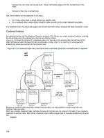
The advantages and disadvantages of each kind of testbench type are
shown in Figure 14-3.
Notice that the stimulus only and full testbenches use TextIO. This can

limit their speed if the DUT requires a lot of vector input. However, the
advantages of using TextIO is the ease of changing the input data. No re-
compilation step is required to change the stimulus data. All that is re-
quired to make a change to the input stimulus is to change the input file
and restart the simulation.
The simulator-specific testbench is also very easy to change because
it is typically an interpreted command language. Interpreted command
languages don’t need a separate compile step. Updating the command lan-
guage file and reloading it in the simulator is all that is required to make
a change. The price of this flexibility, however, may be slow execution
speed. An interpreted command language doesn’t need to be compiled, but
may not execute fast depending on how many vectors are needed how
quickly. A design that needs a lot of vectors very quickly may be limited
by the speed of the interpreter.
The fast testbench really excels at going fast, but is much more dif-
ficult to change quickly than some of the other testbench types. To make
a change, the vectors must be updated and the testbench recompiled. If
the vector file is large, this process can take an excessive amount of time.
Now that we have discussed testbenches, let’s use one to simulate the
CPU for correctness.
Speed Flexibility Portability
Stimulus Only Slow High High
Full Slow High High
Simulator Specific Medium High Low
Hybrid Medium Medium High
Fast Extremely Fast Low High
Figure 14-3
Testbench
Advantages and
Disadvantages.

349
CPU: RTL Simulation
CPU Simulation
Simulating the CPU design is different from most other entities because
the CPU design doesn’t need much outside stimulus. The memory device
provides the input data for the CPU much as a stimulus file would for
other entities. The CPU reads its program from the memory device. The
CPU need only have the clk signal and reset signal stimulated properly,
and the CPU reads and executes instructions from that point forward.
The only stimulus needed to start the operation of the CPU is a uniform
signal applied to the clk input and a pulse applied to the reset input for
at least 2 clock cycles. This starts the CPU into the reset sequence. After
the reset sequence has been started, the CPU is initialized and starts
executing the CPU instructions from the mem entity.
The CPU is simulated as stimulus only initially to verify that the device
seems to be functioning. More complex testbenches need to be created that
include comparison against a known good result to verify correctness. The
simplest method for doing this is to manually verify the results the first
time, capture the output results, and then use them for comparison later.
The first step in simulating the CPU is to compile all the files that
make up the design into a format that the simulator can use. The com-
piled format is loaded into the simulator, and the simulation is executed.
The ModelSim simulator from Model Technology is used for the simu-
lation process.
The first step in compiling all of the files in the design is to create one
or more libraries to store the compiled data. The default library to store
the compiled data is a library called work. The name work is the logical
name of the library; the physical location of the library can be anywhere.
To create a library, the VLIB command is used as shown here:
vlib work

This creates the work library in the current working directory of the
current disk. After the library has been created, the VHDL source files for
the design can be compiled into the target library. To compile each of the
files, the VCOM command must be run either from the GUI (Graphical User
Interface) or from the command line. Most of the operations of the simu-
lator have a GUI method of performing the command line command. This
allows casual users as well as expert users to effectively use the simula-
tor. Normally, casual users use the GUI and experts use the command line
and script interface.
Chapter Fourteen
350
Figure 14-4
Compile VHDL
Source Dialog Box.
To compile a file from the GUI, the file is selected in the compile dialog
box as shown in Figure 14-4.
The GUI includes a file browser that allows the designer to select the
files to compile and then click the Compile button to compile the file.
To compile a file from the command line interface, the following command
is issued:
vcom cpu_lib.vhd
This checks that the VHDL syntax is correct and converts the VHDL
syntax to the binary format needed to simulate the design. Following is a
complete script that compiles all of the files in the proper order:
vcom cpu_lib.vhd
vcom alu.vhd
vcom comp.vhd
vcom reg.vhd
vcom shift.vhd
vcom control.vhd

351
CPU: RTL Simulation
Figure 14-5
Waveform Display of
the Reset Sequence.
vcom regarray.vhd
vcom trireg.vhd
vcom cpu.vhd
vcom mem.vhd
vcom top.vhd
After all of the files have been compiled, the design can be loaded into
the simulator for verification. This can be initiated from the GUI or from
the command line with the following command:
vsim -lib work top behave
This command specifies the library (work), entity (top), and architecture
(behave) or configuration to simulate. After the design has been loaded,
the simulator needs stimulus for the design and specification of what data
to monitor. For this simulation, the current_state, the memory interface,
program counter, and other signals are monitored. Figure 14-5 shows a
waveform display of the reset sequence of the CPU.
From this display, we can verify that the CPU is functioning properly.
At time 0, the reset signal is set to a ‘1’ value, which puts the CPU into
state reset1, the first state of the reset sequence. After the reset signal
is set to ‘0’, the CPU can begin performing the reset sequence. The two
most interesting signals to examine are current_state and next_state.
Notice that, while the reset input is a ‘1’, the CPU remains in state
reset1. After signal reset is set to a ‘0’, on the next rising edge of signal
clock, current_state advances to state reset2.
Each clock rising edge after that causes the CPU to advance to the next
state. At state reset3, the data bus receives the value 0000 to be used as

the starting address for the first instruction. At state reset4, register
Chapter Fourteen
352
Figure 14-6
Waveform Display
after the Reset
Sequence Has
Completed.
addreg
is loaded with the data bus value so that the 0000 value can be
used to drive the addr bus. At state reset5, the data bus is driven with
the instruction data from component mem at address 0. This data is then
loaded into register instrreg in reset6 so that the control entity can use
the instruction contents.
The next state after reset6 is the first execution step of the instruction
that was just fetched from the memory. Looking back at the description
of the
mem entity, we can see that the first instruction loads register 1 with
the source address of the copy operation. Figure 14-6 shows the waveform
display after the reset sequence has completed and the first instruction
has started to execute.
This instruction is a LoadI (Load Immediate) instruction that uses two
words of the memory. The instruction is shown here:
LoadI 1, #
10
The first word of the instruction specifies the behavior of the instruction,
and the second specifies the data to be loaded into the register specified
by the instruction. This instruction first puts the program counter value
to the data bus so that the value can be incremented. The program
counter is then able to read the second word of the instruction that contains

the data to be loaded into reg 1.
During state
execute, the program counter is incremented and the
incremented value can be found as the output of the ALU aluout. During
states loadi2, loadi3, and loadi4, this value is transferred to register
addreg and data is read from mem entity in state loadi5. During state
loadi6, data from memory is loaded into register 1.
353
CPU: RTL Simulation
Figure 14-7
A Waveform Display
Showing the Store
Instruction.
After the load instruction has executed all of the states, to complete the
load instruction, the CPU advances to a set of states that increments
the program counter register to point to the next instruction.
The CPU performs three load instructions to load the proper CPU
registers before the block copy can proceed. A final load instruction is
performed which loads the value to be copied into register 3. At this point,
the CPU program counter is pointing to address 7, a store instruction.
This instruction uses the address in reg 2 to store the value in reg 3 to
the new location. A waveform display showing the store instruction is
shown in Figure 14-7.
During state execute, the value of reg2 is read to the data bus where it
is copied to the address register in state store2. During store3, register
array (3) drives the data bus with the data to be stored. During state
store4, the value is written to the mem address.
After the store instruction is completed, the CPU checks to see if the
block copy operation has completed. This is accomplished by the instruction
at location 8, which branches back to instruction 00 if reg 1 is greater than

reg 6. This instruction execution is shown Figure 14-8.
The first step is to read the value of register 1. This value is stored to
register
opreg during state bgti2. Next, the value of reg6 is read and a
comparison is performed. Notice that signal compout stays a ‘0’ value
because the greater than operation failed; therefore, the branch operation
is be performed.
This set of instructions is performed a number of times until the
source array is copied to the destination array. The source array is shown
in Figure 14-9.
The array starts at location 16 and continues to location 31. The pattern
stored in the source array is a very simple one that starts at 1 and ends
Chapter Fourteen
354
Figure 14-8
Branch Instruction
execution.
Figure 14-9
The Source Array.
355
CPU: RTL Simulation
Figure 14-10
The Destination Array
Before the Copy
Operation Has
Completed.
at 16. Figure 14-10 shows the destination array before the copy operation
has completed.
The destination array starts at location 48 and ends at location 63. The
destination array is shown after two copy operations have been performed.

Notice that location 48 has the first value, and location 49 has the second
value. A complete simulation run completely copies one array to another.
All of the examples that allow the reader to duplicate the simulation of
the CPU are found on the CD that comes with this book.
SUMMARY
In this chapter, we examined what was necessary to perform a functional
verification of the CPU design and walked through one loop of the block
copy operation CPU simulation. In the next chapter, we synthesize the
CPU description to a target FPGA device for implementation.
This page intentionally left blank.