Financial Engineering PrinciplesA Unified Theory for Financial Product Analysis and Valuation phần 2 ppt
Bạn đang xem bản rút gọn của tài liệu. Xem và tải ngay bản đầy đủ của tài liệu tại đây (541.06 KB, 31 trang )
by purchasing goods or services or other investment vehicles, including equi-
ties, bonds, real estate, precious metals, or even other currencies.
A currency typically is thought of as a unit of implied value. I say
“implied value” because in contrast with times past, today’s coins and paper
money are rarely worth the materials used to make them and they tend not
to be backed by anything other than faith and trust in the government mint-
ing or printing the money. For example, in ancient Rome, the value of a par-
ticular coin was typically its intrinsic value—that is, its value in its natural
form of silver or gold. And over varying periods of time, the United States
and other countries relied on linking national currencies to gold and/or sil-
ver where paper money was sometimes said to be backed by gold or subject
to a gold standard—that is, actual reserves of gold were set aside in support
of outstanding supplies of currency. The use of gold as a centerpiece of cur-
rency valuation pretty much faded from any practical meaning in 1971.
Since the physical manifestation of a currency (in the form of notes or
coins) is typically the responsibility of national governments, the judgment of
how sound a given currency may be generally is regarded as inexorably linked
to how sound the respective government is regarded as being. Rightly or
wrongly, national currencies today typically are backed by not much more than
the confidence and expectation that when a currency (or one of its derivatives,
as with a check or credit card) is presented for payment, it typically will be
accepted. As we will see, while the whole notion of currencies being backed
by precious metals has faded as a way of conveying a sense of discipline or
credibility, some currencies in the world are backed by other currencies, for
reasons not too dissimilar from historical incentives for using gold or silver.
While the value of a stock or bond generally is expressed in units of a
currency (e.g., a share of IBM stock costs $57 or a share of Société Generale
stock costs 23), a way to value a currency at a particular time is to mea-
sure how much of a good or service it can purchase. For example, 40 years
Products 7
TABLE 1.1 Similarities and Differences of Equities and Bonds
Equities Bonds
Entitles holder to vote √
Entitles holder to a preferable
ranking in default √
Predetermined life span √
Has a price √√
Has a yield √√
May pay a coupon √
May pay a dividend √
01_200306_CH01/Beaumont 8/15/03 3:50 PM Page 7
TLFeBOOK
ago $1 probably could have been exchanged for 100 pencils. Today, how-
ever, 100 pencils cost more than $1. Accordingly, we could say that the value
of the dollar has depreciated; it buys fewer pencils today than it did 40 years
ago. To express this another way, today we have to spend more than $1 to
obtain the same 100 pencils that people previously spent just $1 to obtain.
Spending more money to purchase the same goods is a classic definition of
inflation, and inflation certainly can contribute to a currency’s depreciation
(weakening relative to another currency). Conversely, deflation is when the
same amount of money buys more of a good than it did previously, and this
can contribute to the appreciation (strengthening relative to another cur-
rency) of a currency. Deflation may occur when there is a technological
advancement with how a good or service is created or provided, or when
there is a surge in the productivity (a measure of efficiency) involved with
the creation of a good or providing of a service.
Another way to value a currency is by how many units of some other
currency it can obtain. An exchange rate is defined simply as being the mea-
sure of one currency’s value relative to another’s. Yet while this simple def-
inition of an exchange rate may be true, it is not very satisfying. Exchange
rates generally tend to vary over time; what influences how one currency will
trade in relation to another? Well, no one really knows precisely, but a cou-
ple of theories have their particular devotees, and they are worth mention-
ing here. Two of the better-known theories applied to exchange rate pricing
include the theory of interest rate parity and purchasing power parity the-
ory.
INTEREST RATE PARITY
Assume that the annual rate of interest in country X is 5 percent and that
the annual rate of interest in country Y is 10 percent. Clearly, all else being
equal, investors in country X would rather have money in country Y since
they are able to earn more basis points, or bps (1% is equal to 100 bps), in
country Y relative to what they are able to earn at home. Specifically, the
interest rate differential (the difference between two yields, expressed in basis
points) is such that investors are picking up an additional 500 basis points
of yield. However, by investing money outside of their home country,
investors are taking on exchange rate risk. To earn the rate of interest being
offered in country Y, investors first have to convert their country X currency
into country Y currency. At the end of the investment horizon (e.g., one year),
international investors may well have earned more money via a rate of inter-
est higher than what was available at home, but those gains might be greatly
affected (perhaps even entirely eliminated) by swings in the value of respec-
tive currencies. The value of currency Y could fall by a large amount rela-
8 PRODUCTS, CASH FLOWS, AND CREDIT
01_200306_CH01/Beaumont 8/15/03 3:50 PM Page 8
TLFeBOOK
tive to currency X over one year, and this means that less of currency X is
recovered.
Indeed, the theory of interest rate parity essentially argues that on a fully
hedged basis, any differential that exists between the interest rates of two
countries will be eliminated by the differential in exchange rates between
those two countries. Continuing with the preceding example, if a forward
contract is purchased to exchange currency Y for currency X at the end of
the investment horizon, the pricing embedded in the forward arrangement
will be such that the currency loss on the trade will exactly offset the gain
generated by the interest rate differential. That is, currency Y will be priced
so as to depreciate relative to currency X, and by an equivalent magnitude
of 500 bps. In short, whatever interest rate advantage investors might enjoy
initially will be eliminated by currency depreciation when a strategy is exe-
cuted on a hedged basis.
When currency exposures are left unhedged, countries’ interest rates and
currency values may move in tandem or inversely to other countries’ inter-
est rates and currency values. Given the right timing and scenario, interna-
tional investors could not only benefit from the higher rate of interest
provided by a given market, but at the end of the investment horizon they
might also be able to exchange an appreciated currency for their weaker local
currency. Accordingly, they obtain more of their local currency than they had
at the outset, and this is due to both the higher interest rate and the effect
of having been in a strengthening currency. Nonetheless, many portfolio
managers swear by the offsetting nature of yield spreads and currency moves
and argue that, over time, these variables do manage to catch up to one
another and thus mitigate long-term opportunities of any doubling of ben-
efits in total return when investing in nonlocal currencies. Figure 1.2 illus-
trates this point. As shown, there is a fairly meaningful correlation between
these two series of yield spread and currency values.
In summary, while interest rate differentials may or may not have mean-
ingful correlations with currency moves when currencies are unhedged, on
a fully hedged basis there is no interest rate or currency advantage to be
gained. As is explained in the next chapter, interest rate differentials are a
key dynamic with determining how forward exchange rates (spot exchange
rates priced to a future date) are calculated.
PURCHASING POWER PARITY
Another popular theory to explain exchange rate valuation goes by the name
of purchasing power parity (PPP).
The idea behind PPP is that, over time (and the question of what period
of time is indeed a relevant and oft-debated question), the purchasing ability
Products 9
01_200306_CH01/Beaumont 8/15/03 3:50 PM Page 9
TLFeBOOK
of one currency ought to adjust itself to be more in line with the purchasing
power of another currency. Broadly speaking, in a world where exchange rates
are left free to adjust to market imbalances and disequilibria in a price con-
text, exchange rates can serve as powerful equalizers. For example, if the cur-
rency of country X was quite strong relative to country Y, then this would
suggest that on a relative basis, the prices within country Y are perceived to
be lower to consumers in country X. Accordingly, as the theory goes, since
consumers in country X buy more of the goods in country Y (because they
are cheaper) and eventually bid those prices higher (due to greater demand),
an equalization eventually will materialize whereby relative prices of goods in
countries X and Y become more aligned on an exchange rate–adjusted basis.
Although certainly to be taken with a grain of salt, Economist magazine
occasionally updates a survey whereby it considers the price of a McDonald’s
Big Mac on a global basis. Specifically, a Big Mac price in local currency (as
in yen for Japan) is divided by the price for a Big Mac in the United States
(upon conversion of yen into dollars). This result is termed “purchasing power
parity,” and when compared to respective actual dollar exchange rates, an
over- or undervaluation of a currency versus the dollar is obtained. The pre-
sumption is that a Big Mac is a relatively homogeneous product type and
accordingly represents a meaningful point of reference. A rather essential (and
perhaps heroic) assumption to this (or any other comparable PPP exercise)
is that all of the ingredients that go into making a Big Mac are accessible in
10 PRODUCTS, CASH FLOWS, AND CREDIT
–80
–130
Spread
1.10
1.00
Euro/USD
FIGURE 1.2 Yield spread between 10-year German and U.S. government bonds and
the euro-to-dollar exchange rate, September 1, 1999, to January 15, 2000.
01_200306_CH01/Beaumont 8/15/03 3:50 PM Page 10
TLFeBOOK
each of the countries where the currencies are being compared. Note that
“equal” in this scenario does not necessarily have to mean that access to
goods (inputs) is 100 percent free of tariffs or any type of trade barrier. If
trade were indeed completely unfettered then this would certainly satisfy the
notion of equally accessible. But if all goods were also subject to the same
barriers to access, this would be equal too, at least in the sense that equal in
this instance means equal barriers. Yet the vast number of trade agreements
that exist globally highlights just how bureaucratic the ideal of free trade can
become even if perceptions (and realities) are such that trade today is gener-
ally at the most free it has ever been. Another important and obvious con-
sideration is that certain inputs might enjoy advantages of proximity. Beef
may be more plentiful in the United States relative to Japan, for example.
The very fact that there is both an interest rate theory to explain cur-
rency phenomenon and a notion of purchasing power parity tells us that
there are at least two different academic approaches to thinking about where
currencies ought to trade relative to one another. No magic keys to unlock-
ing unlimited profitability here! But like any useful theories commonly
applied in any field, here they are popular presumably because they man-
age to shed at least some light on market realities. Generally speaking, mar-
ket participants tend to be a rather pragmatic and results-oriented lot; if
something does not “work,” then its wholesale acceptance and use is not
very likely.
So why is it that neither interest rate parity nor purchasing power par-
ity works perfectly? The answer lies within the question: The markets them-
selves are not perfect. For example, interest rates generally are influenced to
an important degree by national central banks that are trying to guide an
economy in some preferred way. As interest rates can be an important tool
for central banks, these are often subject to the policies dictated by well-
meaning and certainly well-informed people, yet people do make mistakes.
Monetarists believe that one way to eliminate independent judgment of all
kinds (both correct and incorrect) is to allow a country’s monetary policy
to be set by a fixed rule. That is, instead of a country’s money supply being
determined by human and subjective factors, it would be set by a computer
programmed to allow only for a rigid set of money growth parameters.
As to other price realities in the marketplace that may inhibit a smoother
functioning of interest rate or PPP theories, there are a number of consid-
erations, including these three.
1. Quite simply, the supply and demand of various goods around the world
differ by varying degrees, and unique costs can be incurred when spe-
cial efforts are required to make a given good more readily available.
For example, some countries can produce and refine their own oil, while
others are required to import their energy needs.
Products 11
01_200306_CH01/Beaumont 8/15/03 3:50 PM Page 11
TLFeBOOK
2. The cost of some goods in certain countries are subsidized by local gov-
ernments. This extra-market involvement can serve to skew price rela-
tionships across countries. One example of how a government subsidy
can skew a price would be with agricultural products. Debates around
these subsidies can become highly charged exchanges invoking cries of
the need to take care of one’s own domestic producers, to appeal for the
need to develop self-reliant stores of goods so as to limit dependence on
foreign sources. Accordingly, by helping farmers and effectively lower-
ing the costs borne to produce foodstuffs, these savings are said to be
passed along to consumers who enjoy lower-cost items relative to the
price of imported things. Ultimately whether this practice is good or bad
is not likely to be answered here.
3. As alluded to above, tariffs or even total bans on the trade of certain
goods can have a distorting effect on market equilibriums.
There are, of course, many other ways that price anomalies can emerge (e.g.,
with natural disasters). Perhaps this is why the parity theories are most help-
ful when viewed as longer-run concepts.
Is there perhaps a link of some kind between interest rate parity and pur-
chasing power parity? The answer to this question is yes; the link is infla-
tion. An interest rate as defined by the Fischer relation is equal to a real rate
of interest plus expected inflation (as with a measure of CPI or Consumer
Price Index). For example, if an annual nominal interest rate is equal to 6
percent and expected inflation is running at 2.5 percent, then the difference
between these two rates is the real interest rate (3.5 percent). Therefore, infla-
tion is an important factor with interest rate parity dynamics. Similarly, price
levels within countries are affected by inflation phenomena, and so are price
dynamics across countries. Therefore, inflation is an important factor with
PPP dynamics as well. In sum, whether via a mechanism where an interest
rate is viewed as a “price” (as in the price to borrow a particular currency)
or via a mechanism where a particular amount of a currency is the “price”
for obtaining a certain good or service, inflation across countries (or, per-
haps more accurately, inflation differentials across countries) can play an
important role in determining respective currency values.
As of this writing, there are over 50 currencies trading in the world
today.
3
While many of these currencies are well recognized, such as the U.S.
dollar, the Japanese yen, or the United Kingdom’s pound sterling, many are
not as well recognized, as with United Arab Emirates dirhams or Malaysian
ringgits. Although lesser-known currencies may not have the same kind of
recognition as the so-called majors (generally speaking, the currencies of the
12 PRODUCTS, CASH FLOWS, AND CREDIT
3
International Monetary Fund, Representative Exchange Rates for Selected
Currencies, November 1, 2002.
01_200306_CH01/Beaumont 8/15/03 3:50 PM Page 12
TLFeBOOK
Group of Seven, or G-7), lesser-known currencies often have a strong price
correlation with one or more of the majors. To take an extreme case, in the
country of Panama, the national currency is the U.S. dollar. Chapters 3 and
4 will discuss this and other unique currency pricing arrangements further.
The G-7 (and sometimes the Group of Eight if Russia is included) is a
designation given to the seven largest industrialized countries of the world.
Membership includes the United States, Japan, Great Britain, France,
Germany, Italy, and Canada. G-7 meetings generally involve discussions of
economic policy issues. Since France, Germany, and Italy all belong to the
European Union, the currencies of the G-7 are limited to the U.S. dollar, the
pound sterling, Canadian dollar, the Japanese yen, and the euro. The four
most actively traded currencies of the world are the U.S. dollar, pound ster-
ling, yen, and euro.
CHAPTER SUMMARY
This chapter has identified and defined the big three: equities, bonds, and
currencies. The text discussed linkages among equities and bonds in partic-
ular, noting that an equity gives a shareholder the unique right to vote on
matters pertaining to a company while a bond gives a debtholder the unique
right to a senior claim against assets in the event of default. A discussion of
pricing for equities, bonds, and currencies was begun, which is developed
further in a more mathematical context in Chapter 2.
As a parting perspective of the similarities among bonds, equities, and
currencies, it is well to consider if one critical element could serve effectively
to distinguish each of these products. In the case of what makes an equity
Products 13
Equities
Currencies
Absence of right
to vote
Bonds
Absence of
the ability to
print money
Absence of a final maturity date
FIGURE 1.3 Key differences among bonds, equities, and currencies.
01_200306_CH01/Beaumont 8/15/03 3:50 PM Page 13
TLFeBOOK
an equity, the Achilles’ heel is the right to vote that is conveyed in a share
of common stock. Without this right, an equity becomes more of a hybrid
between an equity and a bond. In the case of bonds, a bond without a stated
maturity immediately becomes more of a hybrid between a bond and an
equity. And a country that does not have the ability to print more of its own
money may find its currency treated as more of a hybrid between a currency
and an equity. Figure 1.3 presents these unique qualities graphically. The text
returns time and again to these and other ways of distinguishing among fun-
damental product types.
14 PRODUCTS, CASH FLOWS, AND CREDIT
01_200306_CH01/Beaumont 8/15/03 3:50 PM Page 14
TLFeBOOK
Cash Flows
15
CHAPTER
2
Forwards
&
futures
Options
Spot
Spot
Bonds
If the main thrust of this chapter can be distilled into a single thought, it is
this: Any financial asset can be decomposed into one or more of the fol-
lowing cash flows: spot, forwards and futures, and options. Let us begin with
spot.
“Spot” simply refers to today’s price of an asset. If yesterday’s closing price
for a share of Ford’s equity is listed in today’s Wall Street Journal at $60,
then $60 is Ford’s spot price. If the going rate for the dollar is to exchange
it for 1.10 euros, then 1.10 is the spot rate. And if the price of a three-
month Treasury bill is $983.20, then this is its spot price. Straightforward
stuff, right? Now let us add a little twist.
In the purest of contexts, a spot price refers to the price for an imme-
diate exchange of an asset for its cash value. But in the marketplace, imme-
diate may not be so immediate. In the vernacular of the marketplace, the
sale and purchase of assets takes place at agreed-on settlement dates.
02_200306_CH02/Beaumont 8/15/03 12:41 PM Page 15
TLFeBOOK
For example, a settlement that is agreed to be next day means that the
securities will be exchanged for cash on the next business day (since settle-
ment does not occur on weekends or market holidays). Thus, for an agree-
ment on a Friday to exchange $1,000 dollars for euros at a rate of 1.10 using
next day settlement, the $1,000 would not be physically exchanged for the
1,100 until the following Monday.
Generally speaking, a settlement day is quoted relative to the day that
the trade takes place. Accordingly, a settlement agreement of T plus 3 means
three business days following trade date. There are different conventions for
how settlement is treated depending on where the trade is done (geograph-
ically) and the particular product types concerned.
Pretty easy going thus far if we are willing to accept that the market’s
judgment of a particular asset’s spot price is also its value or true worth (val-
uation above or below the market price of an asset). Yes, there is a distinc-
tion to be made here, and it is an important one. In a nutshell, just because
the market says that the price of an asset is “X” does not have to mean that
we agree that the asset is actually worth that. If we do happen to agree, then
fine; we can step up and buy the asset. In this instance we can say that for
us the market’s price is also the worth of the asset. If we do not happen to
agree with the market, that is fine too; we can sell short the asset if we believe
that its value is above its current price, or we can buy the asset if we believe
its value is below its market price. In either event, we can follow meaning-
ful strategies even when (perhaps especially when) our sense of value is not
precisely in line with the market’s sense of value.
Expanding on these two notions of price and worth, let us now exam-
ine a few of the ways that market practitioners might try to evaluate each.
Broadly speaking, price can be said to be definitional, meaning that it
is devoid of judgment and simply represents the logical outcome of an equa-
tion or market process of supply and demand.
Let us begin with the bond market and with the most basic of financial
instruments, the Treasury bill. If we should happen to purchase a Treasury
bill with three months to maturity, then there is a grand total of two cash
flows: an outflow of cash when we are required to pay for the Treasury bill
at the settlement date and an inflow of cash when we choose to sell the
Treasury bill or when the Treasury bill matures. As long as the sale price or
price at maturity is greater than the price at the time of purchase, we have
made a profit.
A nice property of most fixed income securities is that they mature at
par, meaning a nice round number typically expressed as some multiple of
$1,000. Hence, with the three-month Treasury bill, we know with 100 per-
cent certainty the price we pay for the asset, and if we hold the bill to matu-
rity, we know with 100 percent certainty the amount of money we will get
in three months’ time. We assume here that we are 100 percent confident
16 PRODUCTS, CASH FLOWS, AND CREDIT
02_200306_CH02/Beaumont 8/15/03 12:41 PM Page 16
TLFeBOOK
that the U.S. federal government will not go into default in the next three
months and renege on its debts.
1
If we did in fact believe there was a chance
that the U.S. government might not make good on its obligations, then we
would have to adjust downward our 100 percent recovery assumption at
maturity. But since we are comfortable for the moment with assigning 100
percent probabilities to both of our Treasury bill cash flows, it is possible
for us to state with 100 percent certainty what the total return on our
Treasury bill investment will be.
If we know for some reason that we are not likely to hold the three-
month Treasury bill to maturity (perhaps we will need to sell it after two
months to generate cash for another investment), we can no longer assume
that we can know the value of the second cash flow (the sale price) with 100
percent certainty; the sale price will likely be something other than par, but
what exactly it will be is anyone’s guess. Accordingly, we cannot say with
100 percent certainty what a Treasury bill’s total return will be at the time
of purchase if the bill is going to be sold anytime prior to its maturity date.
Figure 2.1 illustrates this point.
Certainly, if we were to consider what the price of our three-month
Treasury bill were to be one day prior to expiration, we could be pretty con-
fident that its price would be extremely close to par. And in all likelihood
Cash Flows 17
1
If the government were not to make good on its obligations, there would be the
opportunity in the extreme case to explore the sale of government assets or
securing some kind of monetary aid or assistance.
Cash
inflow
Cash
outflow
0
1 month
later
Purchase date.
Cash flow known
with 100% certainty.
2 months
later
3 months
later
Precise cash flow value in between time of
purchase and maturity date cannot be known
with certainty at time of purchase…
3-month Treasury bill
Maturity date.
Cash flow known
with 100% certainty.
Time
FIGURE 2.1 Cash flows of a 3-month Treasury bill.
02_200306_CH02/Beaumont 8/15/03 12:41 PM Page 17
TLFeBOOK
the price of the Treasury bill one day after purchase will be quite close to
the price of the previous day. But the point is that using words like “close”
or “likelihood” simply underscores that we are ultimately talking about
something that is not 100 percent certain. This particular uncertainty is
called the uncertainty of price.
Now let us add another layer of uncertainty regarding bonds. In a
coupon-bearing security with two years to maturity, we will call our uncer-
tainty the uncertainty of reinvestment, that is, the uncertainty of knowing
the interest rate at which coupon cash flows will be reinvested. As Figure
2.2 shows, instead of having a Treasury security with just two cash flows,
we now have six.
As shown, there is a cash outlay at time of purchase, coupons paid at
regular six-month intervals, and the receipt of par and a coupon payment
at maturity; these cash flows can be valued with 100 percent certainty at the
time of purchase, and we assume that this two-year security is held to matu-
rity. But even though we know with certainty what the dollar amount of the
intervening coupon cash flows will be, this is not enough to state at time of
purchase what the overall total return will be with 100 percent certainty. To
better understand why this is the case, let us look at some formulas.
First, for our three-month Treasury bill, the annualized total return is
calculated as follows if the Treasury bill is held to maturity:
Accordingly, for a three-month Treasury bill purchased for $989.20, its
annualized total return is 4.43 percent. The second term, 365/90, is the
annualization term. We assume 365 days in a year (366 for a leap year), and
Cash out Ϫ cash in
Cash in
ϫ
365
90
ϭ Annualized total return
18 PRODUCTS, CASH FLOWS, AND CREDIT
Cash
inflow
Cash
outflow
0
Purchase
12 months later
– Coupon payment
6 months later
– Coupon payment
Time
24 months later
– Coupon and principal
payments
18 months later
– Coupon payment
FIGURE 2.2 Cash flows of a 2-year coupon-bearing Treasury bond.
02_200306_CH02/Beaumont 8/15/03 12:41 PM Page 18
TLFeBOOK
90 days corresponds to the three-month period from the time of purchase
to the maturity date. It is entirely possible to know at the time of purchase
what the total return will be on our Treasury bill. However, if we no longer
assume that the Treasury bill will be held to maturity, the “cash-out” value
is no longer par but must be something else. Since it is not possible to know
with complete certainty what the future price of the Treasury bill will be on
any day prior to its maturity, this uncertainty prevents us from being able
to state a certain total return value prior to the sale date.
What makes the formula a bit more difficult to manage with a two-year
security is that there are more cash flows involved and they all have a time
value that has to be considered. It is material indeed to the matter of total
return how we assume that the coupon received at the six-month point is
treated. When that coupon payment is received, is it stuffed into a mattress,
used to reinvest in a new two-year security, or what? The market’s conven-
tion, rightly or wrongly, is to assume that any coupon cash flows paid prior
to maturity are reinvested for the remaining term to maturity of the under-
lying security and that the coupon is reinvested in an instrument of the same
issuer profile. The term “issuer profile” primarily refers to the quality and
financial standing of the issuer. It also is assumed that the security being pur-
chased with the coupon proceeds has a yield identical to the underlying secu-
rity’s at the time the underlying security was purchased,
2
and has an identical
compounding frequency. “Compounding” refers to the reinvestment of cash
flows and “frequency” refers to how many times per year a coupon-bear-
ing security actually pays a coupon. All coupon-bearing Treasuries pay
coupons on a semiannual basis. The last couple of lines of text give four
explicit assumptions pertaining to how a two-year security is priced by the
market. Obviously, this is no longer the simple and comfortable world of
Treasury bills.
Coupon payments prior to maturity are assumed to be:
1. Reinvested.
2. Reinvested for a term equal to the remaining life of the underlying bond.
3. Reinvested in an identical security type (e.g., Treasury-bill).
4. Reinvested at a yield equal to the yield of the underlying security at the
time it was originally purchased.
Cash Flows 19
2
It would also be acceptable if the cash flow–weighted average of different yields
used for reinvestment were equal the yield of the underlying bond at time of
purchase. In this case, some reinvestment yields could be higher than at time of
original purchase and some could be lower.
02_200306_CH02/Beaumont 8/15/03 12:41 PM Page 19
TLFeBOOK
To help reinforce the notion of just how important reinvested coupons
can be, consider Figure 2.3, which shows a five-year, 6 percent coupon-
bearing bond. Three different reinvestment rates are assumed: 9 percent, 6
percent, and 3 percent. When reinvestment occurs at 6 percent (equal to the
coupon rate), a zero contribution is made to the overall total return.
However, if cash flows can be reinvested at 9 percent, then at the end of five
years an additional 7.6 points ($76 per $1,000 face) of cumulative dollar
value above the 6 percent base case scenarios is returned. By contrast, if rates
are reinvested at 3 percent, then at the end of five years, 6.7 points ($67 per
$1,000 face) of cumulative dollar value is lost relative to the 6 percent base
case scenario.
Figure 2.3 portrays the assumptions being made.
The mathematical expression for the Figure 2.4 is:
The C in the equation is the dollar amount of coupon, and it is equal
to the face amount (F) of the bond times the coupon rate divided by its com-
pounding frequency. The face amount of a bond is the same as the par value
received at maturity. In fact, when a bond first comes to market, face, price,
and par values are all identical because when a bond is launched, the coupon
ϩ
C
11 ϩ Y ր 22
3
ϩ
C & F
11 ϩ Y ր 22
4
ϭ $1,000
Price at time of purchase ϭ
C
(1 ϩ Y ր 2)
1
ϩ
C
(1 ϩ Y ր 2)
2
20 PRODUCTS, CASH FLOWS, AND CREDIT
–8
–6
–4
–2
0
2
12345
4
6
8
Cumulative point values of
reinvested coupon income
relative to 6% base case
Reinvestment at 9%
Reinvestment at 6%
Reinvestment at 3%
Passage of
time
FIGURE 2.3 Effect of reinvestment rates on total return.
02_200306_CH02/Beaumont 8/15/03 12:41 PM Page 20
TLFeBOOK
rate is equal to Y. The Y in the equation is yield, and it is the same value in
each term of the equation. This is equivalent to saying that we expect each
coupon cash flow (except the last two, coupon and principal) to be reinvested
for the remaining life of the underlying security at the yield level prevailing
when the security was originally purchased. Accordingly, the price of a 6 per-
cent coupon-bearing two-year Treasury with a 6 percent yield is $1,000 as
shown in the next equation.
If yield should happen to drop to 5 percent after initial launch, the
coupon rate remains at 6 percent and the price increases to $1,018.81. And
if the yield should happen to rise to 7 percent after launch, the price drops
to 981.63. Hence, price and yield move inversely to one another. Moreover,
by virtue of price’s sensitivity to yield levels (and, hence, reinvestment rates),
a coupon-bearing security’s unhedged total return at maturity is impossible
to pin down at time of purchase. Figure 2.4 confirms this.
Figure 2.5 plots the identical yields from the last equation after revers-
ing the order in which the individual terms are presented. This order rever-
ϩ
$60>2
11 ϩ 6%>22
3
ϩ
$60>2 & $1,000
11 ϩ 6%>22
4
ϭ $1,000
$60>2
11 ϩ 6%>22
1
ϩ
$60>2
11 ϩ 6%>22
2
Cash Flows 21
Cash
inflow
Cash
outflow
0
Purchase
12 months later
– Coupon payment
6 months later
– Coupon payment
To be reinvested for
18 months
To be reinvested for
12 months
To be reinvested for
6 months
Time
24 months later
– Coupon and principal
payments
18 months later
– Coupon payment
All reinvestments assumed to be for the remaining
life of the bond and at the yield that prevailed at the
time of the bond’s purchase.
FIGURE 2.4 Reinvestment requirements of a 2-year coupon-bearing Treasury bond.
02_200306_CH02/Beaumont 8/15/03 12:41 PM Page 21
TLFeBOOK
sal is done simply to achieve a chronological pairing between the timing of
when cash flows are paid and the length of time they are reinvested. Note
how the resulting term structure (a plotting of yields by respective dates) is
perfectly flat.
Note too that when a reinvestment of a coupon cash flow is made, the
new security that is purchased also may be a coupon-bearing security. As
such, it will embody reinvestment risk. Figure 2.6 illustrates this.
Let us now add another layer of uncertainty, called the uncertainty of
credit quality (the uncertainty that a credit may drift to a lower rating or go
into default). Instead of assuming that we have a two-year security issued
by the U.S. Treasury, let us now assume that we have a two-year bond issued
by a U.S. corporation. Unless we are willing to assume that the corporation’s
bond carries the same credit quality as the U.S. government, there are a cou-
ple of things we will want to address. First, we will probably want to change
the value of Y in our equation and make it a higher value to correspond with
the greater risk we are taking on as an investor. And what exactly is that
greater risk? To be blunt, it is the risk that we as investors may not receive
complete (something less than 100 percent), and/or timely payments (pay-
ments made on a date other than formally promised) of all the cash flows
that we have coming to us. In short, there is a risk that the company debt
will become a victim of a distressed or default-related event.
Clearly there are many shades of real and potential credit risks, and these
risks are examined in much more detail in Chapter 3. For the time being,
22 PRODUCTS, CASH FLOWS, AND CREDIT
6%
0 6 12 18 Reinvestment
period
(months)
($60/2)&$1,000 + $60/2 + $60/2 + $60/2 = $1,000
(1 + 6%/2)
4
(1 + 6%/2)
3
(1 + 6%/2)
2
(1 + 6%/2)
1
Yield
FIGURE 2.5 Reinvestment patterns for cash flows of a 2-year coupon-bearing
Treasury bond.
02_200306_CH02/Beaumont 8/15/03 12:41 PM Page 22
TLFeBOOK
we must accept the notion that we can assign credit-linked probabilities to
each of the expected cash flows of any bond. For a two-year Treasury note,
each cash flow can be assigned a 100 percent probability for the high like-
lihood of full and timely payments. For any nongovernmental security, the
Cash Flows 23
Cash
inflow
Cash
outflow
0 Time
Cash
inflow
Cash
outflow
0 Time
Cash
inflow
Cash
outflow
0 Time
Cash
inflow
Cash
outflow
0 Time
FIGURE 2.6 How coupon cash flows of a 2-year Treasury bond give rise to additional
cash flows.
02_200306_CH02/Beaumont 8/15/03 12:41 PM Page 23
TLFeBOOK
probabilities may range between zero and 100 percent. Zero percent? Yes.
In fact, some firms specialize in the trading of so-called distressed debt, which
can include securities with a remaining term to maturity but with little or
no likelihood of making any coupon or principal payments of any kind. A
firm specializing in distressed situations might buy the bad debt (the down-
graded or defaulted securities) with an eye to squeezing some value from the
seizure of the company’s assets. Bad debt buyers also might be able to
reschedule a portion of the outstanding sums owed under terms acceptable
to all those involved.
If we go back to the formula for pricing a two-year Treasury note, we
will most certainly want to make some adjustments to identify the price of
a two-year non-Treasury issue. To compensate for the added risk associated
with a non-Treasury bond we will want a higher coupon paid out to us
—
we will want a coupon payment above C. And since a coupon rate is equal
to Y at the time a bond is first sold, a higher coupon means that we are
demanding a higher Y as well.
To transform the formula for a two-year Treasury
—
from something that is Treasury-specific into something that is relevant for
non-Treasury bonds, we can say that Y
i
represents the yield of a like-matu-
rity Treasury bond plus some incremental yield (and hence coupon) that a
non-Treasury bond will have to pay so as to provide the proper incentive to
purchase it. In the bond market, the difference between this incremental yield
and a corresponding Treasury yield is called a yield spread. Rewriting the
price formula, we have:
Since the same number of added basis points that are now included in
Y
i
are included in C, the price of the non-Treasury bond will still be par at
ϩ
C
11 ϩ Y
i
>22
3
ϩ
C & F
11 ϩ Y
i
>22
4
ϭ $1,000
Price ϭ
C
11 ϩ Y
i
>22
1
ϩ
C
11 ϩ Y
i
>22
2
ϩ
C
11 ϩ Y>22
3
ϩ
C & F
11 ϩ Y>22
4
ϭ $1,000
Price ϭ
C
11 ϩ Y>22
1
ϩ
C
11 ϩ Y>22
2
24 PRODUCTS, CASH FLOWS, AND CREDIT
02_200306_CH02/Beaumont 8/15/03 12:41 PM Page 24
TLFeBOOK
the time of original issue
—
at least when it first comes to the marketplace.
Afterwards things change; yield levels are free to rise and fall, and real and
perceived credit risks can become greater or lesser over time. With regard
to credit risks, greater ones will be associated with higher values of Y
i
and
lower ones will translate into lower values of Y
i
.
So far, we have uncovered three uncertainties pertaining to pricing:
1. Uncertainty of price beyond time of original issue.
2. Uncertainty of reinvestment of coupons.
3. Uncertainty of credit quality.
To understand the layering effect, consider Figure 2.7. The first layer,
uncertainty of price, is common to any fixed income security that is sold
prior to maturity. The second layer, uncertainty of reinvestment, is applica-
ble only to coupon-bearing bonds that pay a coupon prior to sale or matu-
rity. And the third layer, uncertainty of credit quality, generally is unique to
those bond issuers that do not have the luxury of legally printing money (i.e.,
that are not a government entity; for more on this, see Chapter 3).
SPOT PRICING FOR BONDS
Unlike equities or currencies, bonds are often as likely to be priced in terms
of a dollar price as in terms of a yield. Thus, we need to differentiate among
a few different types of yields that are of relevance for bonds.
The examples provided earlier made rather generic references to “yield.”
To be more precise, when a yield is calculated for the spot (or present) value
of a bond, that yield commonly is referred to as yield-to-maturity, bond-
equivalent yield, or present yield. There are also current yields (the result of
dividing a bond’s coupon by its current price), and spot yields (yield on bonds
with no cash flows to be made until maturity). Thus, a spot yield could be
Cash Flows 25
Rising uncertainty
Generally when a security is a nongovernmental issue
When a coupon is paid prior to sale or maturity
For any fixed income security
Uncertainty of credit quality
Uncertainty of reinvestment
Uncertainty of price
FIGURE 2.7 Layers of uncertainty among various types of bonds.
02_200306_CH02/Beaumont 8/15/03 12:41 PM Page 25
TLFeBOOK
a yield on a Treasury bill,
3
a yield on a coupon-bearing bond with no remain-
ing coupons to be paid until maturity, or a yield on a zero-coupon bond. In
some instances even a yield on a coupon-bearing bond that has a price of
par may be said to have a spot yield.
4
In fact, for a coupon-bearing bond
whose price is par, its yield is sometimes called a par bond yield. For all of
the yield types cited, annualizing according to U.S. convention is assumed
to occur on the basis of a 365-day year (except for a leap year). Finally, when
an entire yield curve is comprised of par bond yields, it is referred to as a
par bond curve. A yield curve is created when the dots are connected across
the yields of a particular issuer (or class of issuers) when its bonds are plot-
ted by maturity. Figure 2.8 shows a yield curve of Treasury bonds taken from
November 2002.
As shown, the Treasury bond yield curve is upward sloping. That is,
longer-maturity yields are higher than shorter-maturity yields. In fact, more
26 PRODUCTS, CASH FLOWS, AND CREDIT
3
As a money market instrument (a fixed income security with an original term to
maturity of 12 months or less), a Treasury bill also has unique calculations for its
yield that are called “rate of discount” and “money market yield.” A rate of
discount is calculated as price divided by par and then annualized on the basis of
a 360-day year, while a money market yield is calculated as par minus price
divided by par and then annualized on the basis of a 360-day year.
4
The reason why a coupon-bearing bond priced at par is said to have a yield
equivalent to a spot yield is simply a function of algebraic manipulation. Namely,
since a bond’s coupon rate is equal to its yield when the bond is priced at par, and
since its price and face value are equivalent when yield is equal to coupon rate,
letting C = Y and P = F and multiplying through a generic price/yield equation by
1/F (permissible by the distributive property of multiplication) we get 1 = Y/2/(1 +
Y/2)
1
+ Y/2 /(1 + Y/2)
2
+ In short, C drops away.
Time (years)
Yield
0.5
2
4
6
12 5 10 30
FIGURE 2.8 Normal upward-sloping yield curve.
02_200306_CH02/Beaumont 8/15/03 12:41 PM Page 26
TLFeBOOK
often than not, the Treasury bond yield curve typically reflects such a pos-
itive slope.
When a bond is being priced, the same yield value is used to discount
(reduce to a present value) every cash flow from the first coupon received
in six months’ time to the last coupon and face amount received in 2 or even
30 years’ time. Instead of discounting a bond’s cash flows with a single yield,
which would suggest that the market’s yield curve is perfectly flat, why not
discount a bond’s cash flows with more representative yields? Figure 2.9
shows how this might be done.
In actuality, many larger bond investors (e.g., bond funds and invest-
ment banks) make active use of this approach (or a variation thereof) to pric-
ing bonds to perform relative value (the value of Bond A to Bond B)
analysis. That is, if a bond’s market price (calculated by market convention
with a single yield throughout) was lower than its theoretical value (calcu-
lated from an actual yield curve), this would suggest that the bond is actu-
ally trading cheap in the marketplace.
5
Cash Flows 27
Time (years)
Yield
0.5
2
4
6
12 5 10 30
Price = C&F + C + C + C = $1,000
(1 + Y/2) (1 + Y/2) (1 + Y/2) (1 + Y/2)
4 3
2
1
FIGURE 2.9 Using actual yields from a yield curve to calculate a bond’s price.
5
It is important to note that it is theoretically possible for a given bond to remain
“cheap” (or rich) until the day it matures. A more likely scenario is that a bond’s
cheapness and richness will vary over time. Indeed, what many relative value
investors look for is a good amount of variability in a bond’s richness and
cheapness as a precondition for purchasing it on a relative value basis.
02_200306_CH02/Beaumont 8/15/03 12:41 PM Page 27
TLFeBOOK
While there is just one spot price in the world of bonds, there can be a
variety of yields for bonds. Sometimes these different terms for yield apply
to a single value. For example, for a coupon-bearing bond priced at par, its
yield-to-maturity, current yield, and par bond yield are all the same value.
As previously stated, a yield spread is the difference between the yield
of a nonbenchmark security and a benchmark security, and it is expressed
in basis points.
Therefore, any one of the following things might cause a spread to nar-
row or become smaller (where the opposite event would cause it to widen
or become larger):
A. If the yield of the nonbenchmark (YNB) issue were to . . .
i. . . . decline while the yield of the benchmark (YB) issue were to
remain unchanged
ii. . . .rise while the YB rose by more
iii. . . . remain unchanged while the YB rose
B. If the yield of the benchmark issue (YB) were to . . .
i. . . . rise while the yield of the nonbenchmark (YNB) issue remained
unchanged
ii. . . . decline while the YNB fell by more
iii. . . . remain unchanged while the YNB fell
Thus, the driving force(s) behind a change in spread can be attributable
to the nonbenchmark, the benchmark, or a combination of both.
Accordingly, investors using spreads to identify relative value must keep these
contributory factors in mind.
Regarding spreads generally, while certainly of some value as a single sta-
tic measure, they are more typically regarded by fixed income investors as
having value in a dynamic context. At the very least, a single spread measure
communicates whether the nonbenchmark security is trading rich (at a lower
yield) or cheap (at a higher yield) to the benchmark security. Since the bench-
mark yield is usually subtracted from the nonbenchmark yield, a positive yield
spread suggests that the nonbenchmark is trading cheap to the benchmark
security, and a negative yield spread suggests that it is trading rich to the
benchmark security. To say much beyond this in a strategy-creation context
with the benefit of only one data point (the one spread value) is rather diffi-
cult. More could be said with the benefit of additional data points.
For example, if today’s spread value is 50 basis points (bps), and we
know that over the past four weeks the spread has ranged between 50 bps
Yield of nonbenchmark Ϫ Yield of benchmark ϭ Spread in basis points
28 PRODUCTS, CASH FLOWS, AND CREDIT
02_200306_CH02/Beaumont 8/15/03 12:41 PM Page 28
TLFeBOOK
and 82 bps, then we might say that the nonbenchmark security is at the
richer (narrower) end of the range of where it has traded relative to the
benchmark issue. If today’s spread value were 82 bps, then we might say
that the nonbenchmark security is at the cheaper (wider) end of the range
of where it has been trading. These types of observations can be of great
value to fixed income investors when trying to decipher market trends and
potential opportunities. Yet even for a measure as simple as the difference
between two yields, some basic analysis might very well be appropriate. A
spread might change from day to day for any number of reasons. Many bond
fund managers work to know when and how to trade around these various
changes.
Cash Flows 29
Spot
Equities
Now we can begin listing similarities and differences between equities and
bonds. Equities differ from bonds since they have no predetermined matu-
rity. Equities are similar to bonds since many equities pay dividends, just as
most bonds pay coupons. However, dividends of equities generally tend to
be of lower dollar amounts relative to coupons of bonds, and dividend
amounts paid may vary over time in line with the company’s profitability
and dividend-paying philosophy; the terms of a bond’s coupon payments typ-
ically are set from the beginning. And while not typical, a company might
choose to skip a dividend payment on its equity and without legal conse-
quences, while a skipped coupon payment on a bond is generally sufficient
to initiate immediate concerns regarding a company’s ongoing viability.
6
Occasionally a company may decide to skip a dividend payment altogether,
with the decision having nothing to do with the problems in the company;
there may simply be some accounting incentives for it, for example.
Otherwise, in the United States, bonds typically pay coupons on a semian-
nual basis while equities tend to pay dividends on a quarterly basis. Figure
2.10 is tailored to equities.
6
Terms and conditions of certain preferred equities may impose strict guidelines on
dividend policies that firms are expected to follow.
02_200306_CH02/Beaumont 8/15/03 12:41 PM Page 29
TLFeBOOK
We need to think not only about probabilities related to the nature and
size of future dividends, but also about what to assume for the end price of
an equity purchase. At least among the so-called blue chip (stocks of strong
and well-established companies with reputations for paying dividends over
a variety of market cycles) equities, investors tend to rest pretty comfortably
with the assumption that regular and timely dividend payments will be made
(just as with the debt instruments issued by blue chip corporations).
How can an investor attempt to divine an end price of an equity? There
are formulas available to assist with answering this question, one of which
is called the expected growth in dividends formula. As the name implies, a
forecast of future dividends is required, and such a forecast typically is made
with consideration of expectations of future earnings.
The expected growth in dividends approach to divining a future price
for an equity is expressed as
While this formula may provide some rudimentary guidance on future
price behavior, it falls short of the world of bonds where at least a final matu-
rity price is prespecified.
Perhaps because of the more open-ended matter of determining what an
equity’s price ought to be, there tends to be less of a focus on using quanti-
Expected dividend1s2per share
Cost of equity 1%2Ϫ Expected growth rate of dividend1s21% 2
Expected future price per share ϭ
30 PRODUCTS, CASH FLOWS, AND CREDIT
Cash
inflow
Cash
outflow
0
6 months later
Dividend payment
3 months later
Dividend payment
Price at sale
9 months later
Dividend payment
12 months later
Dividend payment
Note: Dividend payment amounts
may vary from quarter to quarter.
Purchase
– Cash flow known
with 100%
certainty
FIGURE 2.10 Cash flows of a typical equity.
02_200306_CH02/Beaumont 8/15/03 12:41 PM Page 30
TLFeBOOK
tative valuation methods with equities in favor of more qualitative measures.
7
For example, some equity analysts assign great value to determining an
equity’s book value and then forecasting an appropriate multiple for that
book value. Book value is defined as the current value of assets on a com-
pany’s balance sheet according to its accounting conventions, and the term
“multiple” is simply a reference to how many times higher the book value
could trade as an actual market price. For an equity with a $10 per share
book value that an analyst believes should trade at a multiple of eight within
the span of a year, the forecast is for a market value of $80 per share. The
decision to assign a multiple of 8 instead of 4 or 20 may stem from any-
thing ranging from an analyst’s gut feeling to an extensive analysis of a com-
pany’s overall standing relative to peer groups. Other valuation methods
might include analysis of an equity’s price relative to its earnings outlook,
or even technical analysis, which involves charting an equity’s past price
behavior to extrapolate what future price patterns may actually look like.
Investors typically buy bonds for different reasons than why they buy
equities. For example, an investor who is predisposed to a Treasury bond is
likely to be someone who wants the predictability and safety that the
Treasury bond represents. An investor who is predisposed to the equity of
a given issuer (as opposed to the debt of that issuer) is likely to be someone
who is comfortable with the risk and uncertainty of what its price will be
in two years’ time or even two months’ time.
There are some pretty clear expectations about price patterns and
behavior of bonds; in the equity arena, price boundaries are less well delin-
eated. As two significant implications of this observation, equities tend to
experience much greater price action (or volatility) relative to bonds, and
the less constrained (and greater potential) for experiencing upside perfor-
mance would be more likely linked with equities as opposed to bonds (at
least as long as the longer-run economic backdrop is such that the underly-
ing economy itself is growing). Both of these expectations hold up rather well
on a historical basis.
Cash Flows 31
7
I do not mean to detract from the rigor of analysis that often accompanies a
qualitative approach. The point is simply that a key forecast (or set of forecasts) is
required (often pertaining to the expected behavior of future dividends and/or
earnings), and this, by definition, requires cash flow assumptions to be made. This
forecasting requirement is in contrast to the cash flow profile of a Treasury note
where all expected distributions are known at time of purchase.
02_200306_CH02/Beaumont 8/15/03 12:41 PM Page 31
TLFeBOOK