Financial Engineering PrinciplesA Unified Theory for Financial Product Analysis and Valuation phần 3 potx
Bạn đang xem bản rút gọn của tài liệu. Xem và tải ngay bản đầy đủ của tài liệu tại đây (556.31 KB, 31 trang )
and current yield are identical. Further, current yield does not have nearly the
price sensitivity as yield to maturity. Again, this is explained by current yield’s
focus on just the coupon return component of a bond. Since current yield does
not require any assumptions pertaining to the ultimate maturity of the security
in question, it is readily applied to a variety of nonfixed income securities.
Let us pause here to consider the simple case of a six-month forward
on a five-year par bond. Assume that the forward begins one day after a
coupon has been paid and ends the day a coupon is to be paid. Figure 2.13
illustrates the different roles of a risk-free rate (R) and current yield (Y
c
).
As shown, one trajectory is generated with R and another with Y
c
.
Clearly, the purchaser of the forward ought not to be required to pay the
seller’s opportunity cost (calculated with R) on top of the full price (clean
price plus accrued interest) of the underlying spot security. Accordingly, Y
c
is subtracted from R, and the resulting price formula becomes:
for a forward clean price calculation.
For a forward dirty price calculation, we have:
F
d
ϭ S
d
(1 ϩ T (R Ϫ Y
c
)) + A
f
,
where
F
d
ϭ the full or dirty price of the forward (clean price plus accrued
interest)
S
d
ϭ the full or dirty price of the underlying spot (clean price plus
accrued interest)
A
f
ϭ the accrued interest on the forward at expiration of the forward
The equation bears a very close resemblance to the forward formula pre-
sented earlier as F ϭ S (1 ϩ RT). Indeed, with the simplifying assumption that
T ϭ 0, F
d
reduces to S
d
ϩ A
f
. In other words, if settlement is immediate rather
F ϭ S11 ϩ T1R Ϫ Y
c
22
38 PRODUCTS, CASH FLOWS, AND CREDIT
TABLE 2.1
Comparisons of Yield-to-Maturity and Current Yield for
a Semiannual 6% Coupon 2-Year Bond
Price Yield-to-Maturity (%) Current Yield (%)
102 4.94 5.88
100 6.00 6.00
98 7.08 6.12
02_200306_CH02/Beaumont 8/15/03 12:41 PM Page 38
TLFeBOOK
than sometime in the future, F
d
ϭ S
d
since A
f
is nothing more than the accrued
interest (if any) associated with an immediate purchase and settlement.
Inserting values from Figure 2.13 into the equation, we have:
F
d
ϭ 100 (1 ϩ 1/2 (3% Ϫ 5%)) ϩ 5% ϫ 100 ϫ 1/2 ϭ 101.5,
and 101.5 represents an annualized 3 percent rate of return (opportunity
cost) for the seller of the forward.
Clearly it is the relationship between Y
c
and R that determines if F Ͼ S,
F Ͻ S, or F ϭ S (where F and S denote respective clean prices). We already
know that when there are no intervening cash flows F is simply S (1 ϩ RT),
and we would generally expect F Ͼ S since we expect S, R, and T to be pos-
itive values. But for securities that pay intervening cash flows, S will be equal
to F when Y
c
ϭ R; F will be less than S when Y
c
Ͼ R; and F will be greater
than S only when R Ͼ Y
c
. In the vernacular of the marketplace, the case of
Y
c
Ͼ R is termed positive carry and the case of Y
c
Ͻ R is termed negative
carry. Since R is the short-term rate of financing and Y
c
is a longer-term yield
associated with a bond, positive carry generally prevails when the yield curve
has a positive or upward slope, as it historically has exhibited.
Cash Flows 39
Price
Time
102.5 = 100 + 100 * 5% * 1/2
101.5 = 100 + 100 * 3% * 1/2
101.5 – 102.5 = –1.0
100.0 – 1.0 = 99.0 =
F
,
where
F
is the clean
forward price
Of course, these
particular prices
may or may not
actually prevail in
6 months’ time…
Y
c
trajectory (5%)
R
trajectory (3%)
Coupon
payment date
Coupon payment
date and forward
expiration date
6-month forward
is purchased
100
FIGURE 2.13 Relationship between Y
c
and R over time.
02_200306_CH02/Beaumont 8/15/03 12:41 PM Page 39
TLFeBOOK
For the case where the term of a forward lasts over a series of coupon
payments, it may be easier to see why Y
c
is subtracted from R. Since a for-
ward involves the commitment to purchase a security at a future point in
time, a forward “leaps” over a span of time defined as the difference
between the date the forward is purchased and the date it expires. When the
forward expires, its purchaser takes ownership of any underlying spot secu-
rity and pays the previously agreed forward price. Figure 2.14 depicts this
scenario. As shown, the forward leaps over the three separate coupon cash
flows; the purchaser does not receive these cash flows since he does not actu-
ally take ownership of the underlying spot until the forward expires. And
since the holder of the forward will not receive these intervening cash flows,
he ought not to pay for them. As discussed, the spot price of a coupon-bear-
ing bond embodies an expectation of the coupon actually being paid.
Accordingly, when calculating the forward value of a security that generates
cash flows, it is necessary to adjust for the value of any cash flows that are
paid and reinvested over the life of the forward itself.
Bonds are unique relative to equities and currencies (and all other types
of assets) since they are priced both in terms of dollar prices and in terms
of yields (or yield spreads). Now, we must discuss how a forward yield of a
bond is calculated. To do this, let us use a real-world scenario. Let us assume
that an investor is trying to decide between (a) buying two consecutive six-
month Treasury bills and (b) buying one 12-month Treasury bill. Both
investments involve a 12-month horizon, and we assume that our investor
intends to hold any purchased securities until they mature. Should our
investor pick strategy (a) or strategy (b)? To answer this, the investor prob-
40 PRODUCTS, CASH FLOWS, AND CREDIT
Cash flows
Time
Date forward
is purchased
The purchaser of a forward does not receive
the cash flows paid over the life of the
forward and ought not to pay for them.
Date forward expires and
previously agreed forward
price is paid for forward’s
underlying spot
FIGURE 2.14 Relationship between forwards and ownership of intervening cash flows.
02_200306_CH02/Beaumont 8/15/03 12:41 PM Page 40
TLFeBOOK
ably will want some indication of when and how strategy (a) will break even
relative to strategy (b). That is, when and how does the investor become
indifferent between strategy (a) and (b) in terms of their respective returns?
Calculating a single forward rate can help us to answer this question.
To ignore, just for a moment, the consideration of compounding, assume
that the yield on a one-year Treasury bill is 5 percent and that the yield on
a six-month Treasury bill is 4.75 percent. Since we want to know what the
yield on the second six-month Treasury bill will have to be to earn an equiv-
alent of 5 percent, we can simply solve for x with
5% ϭ (4.75% + x)/2.
Rearranging, we have
x ϭ 10% Ϫ 4.75% ϭ 5.25%.
Therefore, to be indifferent between two successive six-month Treasury
bills or one 12-month Treasury bill, the second six-month Treasury bill
would have to yield at least 5.25 percent. Sometimes this yield is referred to
as a hurdle rate, because a reinvestment at a rate less than this will not be
as rewarding as a 12-month Treasury bill. Now let’s see how the calculation
looks with a more formal forward calculation where compounding is con-
sidered.
The formula for F
6,6
(the first 6 refers to the maturity of the future
Treasury bill in months and the second 6 tells us the forward expiration date
in months) tells us the following: For investors to be indifferent between buy-
ing two consecutive six-month Treasury bills or one 12-month Treasury bill,
they will need to buy the second six-month Treasury bill at a minimum yield
of 5.25 percent. Will six-month Treasury bill yields be at 5.25 percent in six
months’ time? Who knows? But investors may have a particular view on the
matter. For example, if monetary authorities (central bank officials) are in
an easing mode with monetary policy and short-term interest rates are
expected to fall (such that a six-month Treasury bill yield of less than 5.25
percent looks likely), then a 12-month Treasury bill investment would
ϭ 5.25%
F
6,6
ϭ cc
11 ϩ 0.05>22
2
11 ϩ 0.0475>22
1
dϪ 1 dϫ 2
F
6,6
ϭ cc
11 ϩ Y
2
>22
2
11 ϩ Y
1
>22
1
dϪ 1 dϫ 2
Cash Flows 41
02_200306_CH02/Beaumont 8/15/03 12:41 PM Page 41
TLFeBOOK
appear to be the better bet. Yet, the world is an uncertain place, and the for-
ward rate simply helps with thinking about what the world would have to
look like in the future to be indifferent between two (or more) investments.
To take this a step further, let us consider the scenario where investors
would have to be indifferent between buying four six-month Treasury bills
or one two-year coupon-bearing Treasury bond. We already know that the
first six-month Treasury bill is yielding 4.75 percent, and that the forward
rate on the second six-month Treasury bill is 5.25 percent. Thus, we still need
to calculate a 12-month and an 18-month forward rate on a six-month
Treasury bill. If we assume spot rates for 18 and 24 months are 5.30 per-
cent and 5.50 percent, respectively, then our calculations are:
For investors to be indifferent between buying a two-year Treasury bond
at 5.5 percent and successive six-month Treasury bills (assuming that the
coupon cash flows of the two-year Treasury bond are reinvested at 5.5 per-
cent every six months), the successive six-month Treasury bills must yield a
minimum of:
5.25 percent 6 months after initial trade
5.90 percent 12 months after initial trade
6.10 percent 18 months after initial trade
Note that 4.75% ϫ .25 ϩ 5.25%ϫ.25 ϩ 5.9%ϫ.25 ϩ 6.1%ϫ.25 ϭ 5.5%.
Again, 5.5 percent is the yield-to-maturity of an existing two-year
Treasury bond.
Each successive calculation of a forward rate explicitly incorporates the
yield of the previous calculation. To emphasize this point, Figure 2.15 repeats
the three calculations.
In brief, in stark contrast to the nominal yield calculations earlier in this
chapter, where the same yield value was used in each and every denomina-
tor where a new cash flow was being discounted (reduced to a present value),
with forward yield calculations a new and different yield is used for every
cash flow. This looping effect, sometimes called bootstrapping, differentiates
a forward yield calculation from a nominal yield calculation.
ϭ 6.10%.
F
6,18
ϭ cc
11 ϩ 0.055>22
4
11 ϩ 0.053>22
3
dϪ 1 dϫ 2
ϭ 5.90%, and
F
6,12
ϭ cc
11 ϩ 0.053>22
3
11 ϩ 0.05>22
2
dϪ 1 dϫ 2
42 PRODUCTS, CASH FLOWS, AND CREDIT
02_200306_CH02/Beaumont 8/15/03 12:41 PM Page 42
TLFeBOOK
Because a single forward yield can be said to embody all of the forward
yields preceding it (stemming from the bootstrapping effect), forward yields
sometimes are said to embody an entire yield curve. The previous equations
show why this is the case.
Table 2.2 constructs three different forward yield curves relative to three
spot curves. Observe that forward rates trade above spot rates when the spot
rate curve is normal or upward sloping; forward rates trade below spot rate
when the spot rate curve is inverted; and the spot curve is equal to the for-
ward curve when the spot rate curve is flat.
The section on bonds and spot discussed nominal yield spreads. In the
context of spot yield spreads, there is obviously no point in calculating the
spread of a benchmark against itself. That is, if a Treasury yield is the bench-
mark yield for calculating yield spreads, a Treasury should not be spread
against itself; the result will always be zero. However, a Treasury forward
spread can be calculated as the forward yield difference between two
Treasuries. Why might such a thing be done?
Again, when a nominal yield spread is calculated, a single yield point on
a par bond curve (as with a 10-year Treasury yield) is subtracted from the
same maturity yield of the security being compared. In sum, two indepen-
dent and comparable points from two nominal yield curves are being com-
pared. In the vernacular of the marketplace, this spread might be referred to
as “the spread to the 10-year Treasury.” However, with a forward curve, if
the underlying spot curve has any shape to it at all (meaning if it is anything
other than flat), the shape of the forward curve will differ from the shape of
the par bond curve. Further, the creation of a forward curve involves a
Cash Flows 43
F
6,6
= (1 + 0.05/2)
2
–1 ϫ 2
(1 + 0.0475/2)
1
= 5.25%
F
6,12
= (1 + 0.053/2)
3
–1 ϫ 2
(1 + 0.05/2)
2
= 5.90%, and
F
6,18
= (1 + 0.055/2)
4
–1 ϫ 2
(1 + 0.053/2)
3
= 6.10%.
FIGURE 2.15 Bootstrapping methodology for building forward rates.
02_200306_CH02/Beaumont 8/15/03 12:41 PM Page 43
TLFeBOOK
process whereby successive yields are dependent on previous yield calcula-
tions; a single forward yield value explicitly incorporates some portion of an
entire par bond yield curve. As such, when a forward yield spread is calcu-
lated between two forward yields, it is not entirely accurate to think of it as
being a spread between two independent points as can be said in a nominal
yield spread calculation. By its very construction, the forward yield embod-
ies the yields all along the relevant portion of a spot curve.
Figure 2.16 presents this discussion graphically. As shown, the bench-
mark reference value for a nominal yield spread calculation is simply taken
from a single point on the curve. The benchmark reference value for a for-
ward yield spread calculation is mathematically derived from points all along
the relevant par bond curve.
If a par bond Treasury curve is used to construct a Treasury forward curve,
then a zero spread value will result when one of the forward yields of a par
bond curve security is spread against its own forward yield level. However,
when a non-par bond Treasury security has its forward yield spread calculated
in reference to forward yield of a par bond issue, the spread difference will likely
be positive.
10
Therefore, one reason why a forward spread might be calculated
between two Treasuries is that this spread gives a measure of the difference
between the forward structure of the par bond Treasury curve versus non-par
bond Treasury issues. This particular spreading of Treasury securities can be
referred to as a measure of a given Treasury yield’s liquidity premium, that is,
44 PRODUCTS, CASH FLOWS, AND CREDIT
10
One reason why non-par bond Treasury issues usually trade at higher forward
yields is that non-par securities are off-the-run securities. An on-the-run Treasury is
the most recently auctioned Treasury security; as such, typically it is the most
liquid and most actively traded. When an on-the-run issue is replaced by some
other newly auctioned Treasury, it becomes an off-the-run security and generally
takes on some kind of liquidity premium. As it becomes increasingly off-the-run,
its liquidity premium tends to grow.
TABLE 2.2 Table Forward Rates under Various Spot Rate Scenarios
Scenario A Scenario B Scenario C
Forward Expiration Spot Forward Spot Forward Spot Forward
6 Month 8.00 /8.00 8.00 /8.00 8.00 /8.00
12 Month 8.25 /8.50 7.75 /7.50 8.00 /8.00
18 Month 8.50 /9.00 7.50 /7.00 8.00 /8.00
24 Month 8.75 /9.50 7.25 /6.50 8.00 /8.00
30 Month 9.00 /10.00 7.00 /6.00 8.00 /8.00
Scenario A: Normal slope spot curve shape (upward sloping)
Scenario B: Inverted slope spot curve
Scenario C: Flat spot curve
02_200306_CH02/Beaumont 8/15/03 12:41 PM Page 44
TLFeBOOK
the risk associated with trading in a non-par bond Treasury that may not always
be as readily available in the market as a par bond issue.
To calculate a forward spread for a non-Treasury security (i.e., a secu-
rity that is not regarded as risk free), a Treasury par bond curve typically is
used as the reference curve to construct a forward curve. The resulting for-
ward spread embodies both a measure of a non-Treasury liquidity premium
and the non-Treasury credit risk.
We conclude this section with Figure 2.17.
BOND FUTURES
Two formulaic modifications are required when going from a bond’s for-
ward price calculation to its futures price calculation. The first key differ-
ence is the incorporation of a bond’s conversion factor. Unlike gold, which
is a standard commodity type, bonds come in many flavors. Some bonds
have shorter maturities than others, higher coupons than others, or fewer
bells and whistles than others, even among Treasury issues (which are the
most actively traded of bond futures). Therefore, a conversion factor is an
attempt to apply a standardized variable to the calculation of all candidates’
spot prices.
11
As shown in the equation on page 46, the clean forward price
Cash Flows 45
Ten years
Yield
Maturity
Par bond curve
Forward curve
FIGURE 2.16 Distinctions between points on and point along par bond and forward curves.
11
A conversion factor is simply a modified forward price for a bond that is eligible
to be an underlying security within a futures contract. As with any bond price, the
necessary variables are price (or yield), coupon, maturity date, and settlement date.
However, the settlement date is assumed to be first day of the month that the
contract is set to expire; the maturity date is assumed to be the first day of the
month that the bond is set to mature rounded down to the nearest quarter (March,
June, September, or December); and the yield is assumed to be 8 percent regardless
of what it may actually be. The dirty price that results is then divided by 100 and
rounded up at the fourth decimal place.
02_200306_CH02/Beaumont 8/15/03 12:41 PM Page 45
TLFeBOOK
of a contract-eligible bond is simply divided by its relevant conversion fac-
tor. When the one bond is flagged as the relevant underlying spot security
for the futures contract (via a process described in Chapter 4), its conver-
sion-adjusted forward price becomes the contract’s price.
The second formula modification required when going from a forward
price calculation to a futures price calculation concerns the fact that a bond
futures contract comes with delivery options. That is, when a bond futures
contract comes to its expiration month, investors who are short the contract
face a number of choices. Recall that at the expiration of a forward or future,
some predetermined amount of an asset is exchanged for cash. Investors who
are long the forward or future pay cash and accept delivery (take owner-
ship) of the asset. Investors who are short the forward or future receive cash
and make delivery (convey ownership) of the asset. With a bond futures con-
tract, the delivery process can take place on any business day of the desig-
nated delivery month, and investors who are short the contract can choose
when delivery is made during that month. This choice (along with others
embedded in the forward contract) has value, as does any asymmetrical deci-
sion-making consideration, and it ought to be incorporated into a bond
future’s price calculation. Chapter 4 discusses the other choices embedded
in a bond futures contract and how these options can be valued.
A bond futures price can be defined as:
where O
d
ϭ the embedded delivery options
CF ϭ the conversion factor
F
d
ϭ 3S 11 ϩ T 1R Ϫ Y
c
22ϩ A
f
Ϫ O
d
4>CF
46 PRODUCTS, CASH FLOWS, AND CREDIT
ForwardsSpot
If the par bond curve
is flat, or if
T
=0
(settlement is
immediate), then the
forward curve . . .
A par bond curve
of spot yields . . .
. . . is identical to a par
bond curve.
. . . is used to construct a
forward yield curve.
FIGURE 2.17 Spot versus forward yield curves.
02_200306_CH02/Beaumont 8/15/03 12:41 PM Page 46
TLFeBOOK
To calculate the forward price of an equity, let us consider IBM at $80.25 a
share. If IBM were not to pay dividends as a matter of corporate policy, then
to calculate a one-year forward price, we would simply multiply the number
of shares being purchased by $80.25 and adjust this by the cost of money for
one year. The formula would be F ϭ S (1 ϩ RT), exactly as with gold or
Treasury bills. However, IBM’s equity does pay a dividend, so the forward price
for IBM must reflect the fact that these dividends are received over the com-
ing year. The formula really does not look that different from what we use for
a coupon-bearing bond; in fact, except for one variable, it is the same. It is
where Y
d
ϭ dividend yield calculated as the sum of expected dividends in
the coming year divided by the underlying equity’s market price.
Precisely how dividends are treated in a forward calculation depends on
such considerations as who the owner of record is at the time that the inten-
tion of declaring a dividend is formally made by the issuer. There is not a
straight-line accretion calculation with equities as there is with coupon-
bearing bonds, and conventions can vary across markets. Nonetheless, in
cases where the dividend is declared and the owner of record is determined,
and this all transpires over a forward’s life span, the accrued dividend fac-
tor is easily accommodated.
CASH-SETTLED EQUITY FUTURES
As with bonds, there are also equity futures. However, unlike bond futures,
which have physical settlement, equity index futures are cash-settled. Physical
settlement of a futures contract means that an actual underlying instrument
(spot) is delivered by investors who are short the contract to investors who
are long the contract, and investors who are long pay for the instrument. When
F ϭ S 11 ϩ T 1R Ϫ Y
d
22
Cash Flows 47
Forwards
& futures
Equities
A minus sign appears in front of O
d
since the delivery options are of
benefit to investors who are short the bond future. Again, more on all this
in Chapter 4.
02_200306_CH02/Beaumont 8/15/03 12:41 PM Page 47
TLFeBOOK
a futures contract is cash-settled, the changing cash value of the underlying
instrument is all that is exchanged, and this is done via the daily marking-to-
market mechanism. In the case of the Standard & Poor’s (S&P) 500 futures
contract, which is composed of 500 individual stocks, the aggregated cash
value of these underlying securities is referenced with daily marks-to-market.
Just as dividend yields may be calculated for individual equities, they
also may be calculated for equity indices. Accordingly, the formula for an
equity index future may be expressed as
where S and Y
d
ϭ market capitalization values (stock price times out-
standing shares) for the equity prices and dividend yields of the com-
panies within the index.
Since dividends for most index futures generally are ignored, there is typ-
ically no price adjustment required for reinvestment cash flow considerations.
Equity futures contracts typically have prices that are rich to (above)
their underlying spot index. One rationale for this is that it would cost
investors a lot of money in commissions to purchase each of the 500 equi-
ties in the S&P 500 individually. Since the S&P future embodies an instan-
taneous portfolio of securities, it commands a premium to its underlying
portfolio of spot instruments. Another consideration is that the futures con-
tract also must reflect relevant costs of carry.
Finally, just as there are delivery options embedded in bond futures con-
tracts that may be exercised by investors who are short the bond future,
unique choices unilaterally accrue to investors who are short certain equity
index futures contracts. Again, just as with bond futures, the S&P 500 equity
future provides investors who are short the contract with choices as to when
a delivery is made during the contract’s delivery month, and these choices
have value. Contributing to the delivery option’s value is the fact that
investors who are short the future can pick the delivery day during the deliv-
ery month. Depending on the marketplace, futures often continue to trade
after the underlying spot market has closed (and may even reopen again in
after-hours trading).
F ϭ S 11 ϩ T 1R Ϫ Y
d
22
48 PRODUCTS, CASH FLOWS, AND CREDIT
Forwards
& futures
Currencies
The calculation for the forward value of an exchange rate is again a mere
02_200306_CH02/Beaumont 8/15/03 12:41 PM Page 48
TLFeBOOK
variation on a theme that we have already seen, and may be expressed as
where R
h
ϭ the home country risk-free rate
R
o
ϭ the other currency’s risk-free rate
For example, if the dollar-euro exchange rate is 0.8613, the three-month
dollar Libor rate (London Inter-bank Offer Rate, or the relevant rate among
banks exchanging euro dollars) is 3.76 percent, and the three-month euro
Libor rate is 4.49 percent, then the three-month forward dollar-euro
exchange rate would be calculated as 0.8597. Observe the change in the dol-
lar versus the euro (of 0.0016) in this time span; this is entirely consistent
with the notion of interest rate parity introduced in Chapter 1. That is, for
a transaction executed on a fully hedged basis, the interest rate gain by invest-
ing in the higher-yielding euro market is offset by the currency loss of
exchanging euros for dollars at the relevant forward rate.
If a Eurorate (not the rate on the euro currency, but the rate on a Libor-
type rate) differential between a given Eurodollar rate and any other euro
rate is positive, then the nondollar currency is said to be a premium currency.
If the Eurorate differential between a given Eurodollar rate and any other
Eurorate is negative, then the nondollar currency is said to be a discount cur-
rency. Table 2.3 shows that at one point, both the pound sterling and
Canadian dollar were discount currencies to the U.S. dollar. Subtracting
Canadian and sterling Eurorates from respective Eurodollar rates gives neg-
ative values.
There is an active forward market in foreign exchange, and it is com-
monly used for hedging purposes. When investors engage in a forward trans-
action, they generally buy or sell a given exchange rate forward. In the last
example, the investor sells forward Canadian dollars for U.S dollars. A for-
F ϭ S 11 ϩ T 1R
h
Ϫ R
o
22
Cash Flows 49
TABLE 2.3 Rates from May 1991
Country 3 Month (%) 6 Month (%) 12 Month (%)
United States 6.0625 6.1875 6.2650
Canada 9.1875 9.2500 9.3750
United Kingdom 11.5625 11.3750 11.2500
02_200306_CH02/Beaumont 8/15/03 12:41 PM Page 49
TLFeBOOK
ward contract commits investors to buy or sell a predetermined amount of
one currency for another currency at a predetermined exchange rate. Thus,
a forward is really nothing more than a mutual agreement to exchange one
commodity for another at a predetermined date and price.
Can investors who want to own Canadian Treasury bills use the for-
ward market to hedge the currency risk? Absolutely!
The Canadian Treasury bills will mature at par, so if the investors want
to buy $1 million Canadian face value of Treasury bills, they ought to sell
forward $1 million Canadian. Since the investment will be fully hedged, it
is possible to state with certainty that the three-month Canadian Treasury
bill will earn
Where did the forward exchange rates come from for this calculation?
From the currency section of a financial newspaper. These forward values
are available for each business day and are expressed in points that are then
combined with relevant spot rates. Table 2.4 provides point values for the
Canadian dollar and the British pound.
The differential in Eurorates between the United States and Canada is
312.5 basis points (bps). With the following calculation, we can convert
U.S./Canadian exchange rates and forward rates into bps.
where
1.1600 ϭ the spot rate
1.1512 ϭ the spot rate adjusted for the proper amount of forward
points
We assume that the Canadian Treasury bill matures in 87 days. Although
316 bps is not precisely equal to the 312.5 bp differential if calculated from
316 basis points ϭ
11.1600 Ϫ 1.15122
1.1512
ϫ
13602
87
5.670% ϭ
1100>1.16002Ϫ 197.90>1.15122
197.90>1.15122
13602
1872
.
50 PRODUCTS, CASH FLOWS, AND CREDIT
TABLE 2.4 Forward Points May 1991
Country 3 Month 6 Month 12 Month
Canada 90 170 290
United Kingdom 230 415 700
02_200306_CH02/Beaumont 8/15/03 12:41 PM Page 50
TLFeBOOK
the yield table, consideration of transaction costs would make it difficult to
structure a worthwhile arbitrage around the 3.5 bp differential.
Finally, note that the return of 5.670 percent is 15 bps above the return
that could be earned on the three-month U.S. Treasury bill. Therefore, given
a choice between a three-month Canadian Treasury bill fully hedged into
U.S dollars earning 5.670 percent and a three-month U.S. Treasury bill earn-
ing 5.520 percent, the fully hedged Canadian Treasury bill appears to be the
better investment.
Rather than compare returns of the above strategy with U.S Treasury
bills, many investors will do the trade only if returns exceed the relevant
Eurodollar rate. In this instance, the fully hedged return would have had to
exceed the three-month Eurodollar rate. Why? Investors who purchase a
Canadian Treasury bill accept a sovereign credit risk, that is, the risk the gov-
ernment of Canada may default on its debt. However, when the three-month
Canadian Treasury bill is combined with a forward contract, another credit
risk appears. In particular, if investors learn in three months that the coun-
terparty to the forward contract will not honor the forward contract,
investors may or may not be concerned. If the Canadian dollar appreciates
over three months, then investors probably would welcome the fact that they
were not locked in at the forward rate. However, if the Canadian dollar depre-
ciates over the three months, then investors could well suffer a dramatic loss.
The counterparty risk of a forward contract is not a sovereign credit risk.
Forward contract risks generally are viewed as a counterparty credit risk. We
can accept this view since banks are the most active players in the currency
forwards marketplace. Though perhaps obvious, an intermediate step
between an unhedged position and a fully hedged strategy is a partially
hedged investment. With a partial hedge, investors are exposed to at least
some upside potential with a trade yet with some downside protection as well.
OPPORTUNITIES WITH CURRENCY FUTURES
Most currency futures are rather straightforward in terms of their delivery
characteristics, where delivery often is made on a single day at the end of
the futures expiration. However, the fact that gaps may exist between the
trading hours of the futures contracts and the underlying spot securities can
give rise to some strategic value.
SUMMARY ON FORWARDS AND FUTURES
This section examined the similarities of forward and future cash flow
types across bonds, equities, and currencies, and discussed the nature of the
Cash Flows 51
02_200306_CH02/Beaumont 8/15/03 12:41 PM Page 51
TLFeBOOK
interrelationship between forwards and futures. Parenthetically, there is a
scenario where the marginal differences between a forward and future actu-
ally could allow for a material preference to be expressed for one over the
other. Namely, since futures necessitate a daily marking-to-market with a
margin account set aside expressly for this purpose, investors who short
bond futures contracts (or contracts that enjoy a strong correlation with
interest rates) versus bond forward contracts can benefit in an environment
of rising interest rates. In particular, as rates rise, the short futures posi-
tion will receive margin since the future’s price is decreasing, and this
greater margin can be reinvested at the higher levels of interest. And if rates
fall, the short futures position will have to post margin, but this financing
can be done at a lower relative cost due to lower levels of interest. Thus,
investors who go long bond futures contracts versus forward contracts are
similarly at a disadvantage.
There can be any number of incentives for doing a trade with a partic-
ular preference for doing it with a forward or future. Some reasons might
include:
Ⅲ Investors’ desire to leapfrog over what may be perceived to be a near-
term period of market choppiness into a predetermined forward trade
date and price
Ⅲ Investors’ belief that current market prices generally look attractive now,
but they may have no immediate cash on hand (or perhaps may expect
cash to be on hand soon) to commit right away to a purchase
Ⅲ Investors’ hope to gain a few extra basis points of total return by actively
exploiting opportunities presented by the repo market via the lending
of particular securities. This is discussed further in Chapter 4.
Table 2.5 presents forward formulas for each of the big three.
52 PRODUCTS, CASH FLOWS, AND CREDIT
Options
We now move to the third leg of the cash flow triangle, options.
Continuing with the idea that each leg of the triangle builds on the other,
the options leg builds on the forward market (which, in turn, was built on
02_200306_CH02/Beaumont 8/15/03 12:41 PM Page 52
TLFeBOOK
the spot market). Therefore, of the five variables generally used to price an
option, we already know three: spot (S), a financing rate (R), and time (T).
The two additional variables needed are strike price and volatility. Strike
price is the reference price of profitability for an option, and an option is
said to have intrinsic value when the difference between a strike price and
an actual market price is a favorable one. Volatility is a statistical measure
of a stock price’s dispersion.
Let us begin our explanation with an option that has just expired. If our
option has expired, several of the five variables cited simply fall away. For
example, time is no longer a relevant variable. Moreover, since there is no
time, there is nothing to be financed over time, so the finance rate variable
is also zero. And finally, there is no volatility to be concerned about because,
again, the game is over. Accordingly, the value of the option is now:
Call option value is equal to S Ϫ K
where
S ϭ the spot value of the underlying security
K ϭ the option’s strike price
The call option value increases as S becomes larger relative to K. Thus,
investors purchase call options when they believe the value of the underly-
ing spot will increase. Accordingly, if the value of S happens to be 102 at
expiration with the strike price set at 100 at the time the option was pur-
chased, then the call’s value is 102 minus 100 ϭ 2.
A put option value is equal to K Ϫ S. Notice the reversal of positions
of S and K relative to a call option’s value. The put option value increases
as S becomes smaller relative to K. Thus, investors purchase put options
when they believe that the value of the underlying spot will decrease.
Now let us look at a scenario for a call’s value prior to expiration. In
this instance, all five variables cited come into play.
The first thing to do is make a substitution. Namely, we need to replace
the S in the equation with an F. T, time, now has value. And since T is rel-
evant, so too is the cost to finance S over a period of time; this is reflected
Cash Flows 53
TABLE 2.5 Forward Formulas for Each of the Big Three
Product Formula
No Cash Flows Cash Flows
Bonds S (1 ϩ RT) S (1 ϩ T (R Ϫ Y
c
))
Equities S (1 ϩ RT) S (1 ϩ T (R Ϫ Y
c
))
Currencies S (1 ϩ T(R
h
ϪR
o
))
02_200306_CH02/Beaumont 8/15/03 12:41 PM Page 53
TLFeBOOK
by R and is embedded along with T within F. And finally, a value for volatil-
ity, V, is also a vital consideration now. Thus, we might now write an equa-
tion for a call’s value to be
Just to be absolutely clear on this point, when we write V as in the last
equation, this variable is to be interpreted as the value of volatility in price
terms (not as a volatility measure expressed as an annualized standard devi-
ation).
12
Since there is a number of option pricing formulas in existence
today, we need not define a price value of volatility in terms of each and
every one of those option valuation calculations. Quite simply, for our pur-
poses, it is sufficient to note that the variables required to calculate a price
value for volatility include R, T, and , where is the annualized standard
deviation of S.
13
On an intuitive level, it would be logical to accept that the price value
of volatility is zero when T ϭ 0, because T being zero means that the option’s
life has come to an end; variability in price (via ) has no meaning. However,
if R is zero, it is still possible for volatility to have a price value. The fact that
there may be no value to borrowing or lending money does not automati-
cally translate into a spot having no volatility (unless, of course, the under-
lying spot happens to be R itself, where R may be the rate on a Treasury bill).
14
Accordingly, a key difference between a forward and an option is the role of
R; R being zero immediately transforms a forward into spot, but an option
remains an option. Rather, the Achilles’ heel of an option is ; being zero
immediately transforms an option into a forward. With ϭ 0 there is no
volatility, hence there is no meaning to a price value of volatility.
Finally, saying that one cash flow type becomes another cash flow type
under various scenarios (i.e., T ϭ 0, or ϭ 0), does not mean that they some-
how magically transform instantaneously into a new product; it simply high-
lights how their new price behavior ought to be expected to reflect the cash
flow profile of the product that shares the same inputs.
Call value ϭ F Ϫ K ϩ V.
54 PRODUCTS, CASH FLOWS, AND CREDIT
12
It is common in some over-the-counter options markets actually to quote options
by their price as expressed in terms of volatility, for example, quoting a given
currency option with a standard three-month maturity at 12 percent.
13
The appendix of this chapter provides a full explanation of volatility definitions,
including volatility’s calculation as an annualized standard deviation of S.
14
Perhaps the most recent real-world example of R being close to (or even below)
zero would be Japan, where short-term rates traded to just under zero percent in
January 2003.
02_200306_CH02/Beaumont 8/15/03 12:41 PM Page 54
TLFeBOOK
Rewriting the above equation for a call option knowing that F ϭ S ϩ
SRT, we have
Call value = S + SRT Ϫ K + V.
If only to help us reinforce the notions discussed thus far as they relate
to the interrelationships of the triangle, let us consider a couple of what-if?
scenarios. For example, what if volatility for whatever reason were to go to
zero? In this instance, the last equation shrinks to
Call value = S + SRT Ϫ K.
And since we know that F ϭ S ϩ SRT, we can rewrite that equation
into an even simpler form as:
Call value = F Ϫ K.
But since K is a fixed value that does not change from the time the option
is first purchased, what the above expression really boils down into is a value
for F. We are now back to the second leg of the triangle. To put this another
way, a key difference between a forward and an option is that prior to expi-
ration, the option requires a price value for V.
For our second what-if? scenario, let us assume that in addition to
volatility being zero, for whatever reason there is also zero cost to borrow
or lend (financing rates are zero). In this instance, call value ϭ S ϩ SRT Ϫ
K ϩ V now shrinks to
Call value = S Ϫ K.
This is because with T and R equal to zero, the entire SRT term drops
out, and of course V drops out because it is zero as well. With the recogni-
tion, once again, that K is a fixed value and does not do very much except
provide us with a reference point relative to S, we now find ourselves back
to the first leg of the triangle. Figure 2.18 presents these interrelationships
graphically.
As another way to evaluate the progressive differences among spot, for-
wards, and options, consider the layering approach shown in Figure 2.19.
The first or bottom layer is spot. If we then add a second layer called cost
of carry, the combination of the first and second layers is a forward. And if
we add a third layer called volatility (with strike price included, though “on
the side,” since it is a constant), the combination of the first, second, and
third layers is an option.
Cash Flows 55
02_200306_CH02/Beaumont 8/15/03 12:41 PM Page 55
TLFeBOOK
As part and parcel of the building-block approach to spot, forwards, and
options, unless there is some unique consideration to be made, the pre-
sumption is that with an efficient marketplace, investors presumably would
be indifferent across these three structures relative to a particular underly-
ing security. In the context of spot versus forwards and futures, the decision
to invest in forwards and futures rather than cash would perhaps be influ-
enced by four things:
56 PRODUCTS, CASH FLOWS, AND CREDIT
Spot
Options
Forwards
F
=
S
(1 +
RT
)
S
Call value =
F
–
K
+
V
=
S
(1 +
RT
)–
K
+
V
When
T
is zero (as at the expiration of an
option), the call option value becomes
S
–
K
. This happens because
F
becomes
S
(see formula for
F
) and
V
drops away;
volatility has no value for a security that has
ceased to trade (as at expiration). In sum,
since
K
is a constant,
S
is the last remaining
variable. If just
V
is zero, then the call option
value prior to expiration is
F
–
K.
Therefore,
F
is differentiated from an option
by
K
and
V
, and
S
is differentiated from an
option by
K, V,
and
RT.
When either
R
or
T
is zero (as
with a zero cost to financing,
or when there is immediate
settlement),
F
=
S
.
Therefore,
F
is differentiated
from
S
by cost of carry (
SRT
)
Special Note
Some market participants state
that the value of an option is
really composed of two parts:
an intrinsic value and a time
value. Intrinsic value is defined
as
F
Ϫ
K
prior to expiration (for
a call option) and as
S
Ϫ
K
at
expiration; all else is time value,
which, by definition, is zero
when
T
= 0 (as at expiration).
FIGURE 2.18 Key interrelationships among spot, forwards, and options.
V
SRT
S
Volatility
Cost of carry
Forwards
Options
Spot
FIGURE 2.19 Layers of distinguishing characteristics among spot, forwards, and options.
02_200306_CH02/Beaumont 8/15/03 12:41 PM Page 56
TLFeBOOK
1. The notion that the forward or future is undervalued or overvalued rela-
tive to cash; that in the eyes of a particular investor, there is a material dif-
ference between the market value of the forward and its actual worth
2. Some kind of investor-specific cash flow or asset consideration where
immediate funds are not desired to be committed; that the deferred exchange
of cash for product provided by the forward or future is desirable
3. The view that something related to SRT is not being priced by the mar-
ket in a way that is consistent with the investor’s view of worth; again,
a material difference between market value and actual worth
4. Some kind of institutional, regulatory, tax, or other extra-market incen-
tive to trade in futures or forwards instead of cash
In the case of investing in an option rather than forwards and futures
or cash, this decision would perhaps be influenced by four things:
1. The notion that the option is undervalued or overvalued relative to for-
wards or futures or cash; that in the eyes of a particular investor, there
is a material difference between the market value of the forward and its
actual worth
2. Some kind of investor-specific cash flow or asset consideration where
the cash outlay of a strategy is desirable; note the difference between
paying S versus S Ϫ K
3. The view that something related to V is not being priced by the market
in a way that is consistent with the investor’s view of worth; again, a
material difference between market value and actual worth
4. Some kind of institutional, regulatory, tax, or other extra-market incen-
tive to trade in options instead of futures or forwards or cash
It is hoped that these illustrations have helped to reinforce the idea of inter-
locking relationships around the cash flow triangle. Often people believe that
these different cash flow types somehow trade within their own unique orbits
and have lives unto themselves. This does not have to be the case at all.
As the concept of volatility is very important for option valuation, the
appendix to this chapter is devoted to the various ways volatility is calcu-
lated. In fact, a principal driver of why various option valuation models exist
is the objective of wanting to capture the dynamics of volatility in the best
possible way. Differences among the various options models that exist today
are found in existing texts on the subject.
15
Cash Flows 57
15
See, for example, John C. Hull, Options, Futures, and Other Derivatives (Saddle-
River. NJ: Prentice Hall, 1989).
02_200306_CH02/Beaumont 8/15/03 12:41 PM Page 57
TLFeBOOK
Because bonds are priced both in terms of dollar price and yield, an overview
of various yield types is appropriate. Just as there are nominal yield spreads and
forward yield spreads, there are also option-adjusted spreads (OASs).
Refer again to the cash flow triangle and the notion of forwards building
on spots, and options, in turn, building on forwards. Recall that a spot spread
is defined as being the difference (in basis points) between two spot yield lev-
els (and being equivalent to a nominal yield spread when the spot curve is a
par bond curve) and that a forward spread is the difference (in bps) between
two forward yield levels derived from the entire relevant portion of respective
spot curves (and where the forward curve is equivalent to a spot curve when
the spot curve is flat). A nominal spread typically reflects a measure of one
security’s richness or cheapness relative to another. Thus, it can be of interest
to investors as a way of comparing one security against another. Similarly, a
forward spread also can be used by investors to compare two securities, par-
ticularly when it would be of interest to incorporate the information contained
within a more complete yield curve (as a forward yield in fact does).
An OAS can be a helpful valuation tool for investors when a security
has optionlike features. Chapter 4 examines such security types in detail.
Here the objective is to introduce an OAS and show how it can be of assis-
tance as a valuation tool for fixed income investors.
If a bond has an option embedded within it, a single security has charac-
teristics of a spot, a forward, and an option all at the same time. We would
expect to pay par for a coupon-bearing bond with an option embedded within
it if it is purchased at time of issue; this “pay-in-full at trade date” feature is
most certainly characteristic of spot. Yet the forward element of the bond is
a “deferred” feature that is characteristic of options. In short, an OAS is
intended to incorporate an explicit consideration of the option component
within a bond (if it has such a component) and to express this as a yield spread
value. The spread is expressed in basis points, as with all types of yield spreads.
Recall the formula for calculating a call option’s value for a bond, equity,
or currency.
O
c
ϭ F Ϫ K ϩ V.
58 PRODUCTS, CASH FLOWS, AND CREDIT
Options
Bonds
02_200306_CH02/Beaumont 8/15/03 12:41 PM Page 58
TLFeBOOK
Table 2.6 compares and contrasts how the formula would be modified
for calculating an OAS as opposed to a call option on a bond.
Consistent with earlier discussions on the interrelationships among spot, for-
wards, and options, if the value of volatility is zero (or if the par bond curve is
flat), then an OAS is the same thing as a forward spread. This is the case because
a zero volatility value is tantamount to asserting that just one forward curve is
of relevance: today’s forward curve. Readers who are familiar with the binom-
inal option model’s “tree” can think of the tree collapsing into a single branch
when the volatility value is zero; the single branch represents the single prevailing
path from today’s spot value to some later forward value. Sometimes investors
deliberately calculate a zero volatility spread (or ZV spread) to see where a given
security sits in relation to its nominal spread, whether the particular security is
embedded with any optionality or not. Simply put, a ZV spread is an OAS cal-
culated with the assumption of volatility being equal to zero. Similarly, if T ϭ
0 (i.e., there is immediate settlement), then volatility has no purpose, and the
OAS and forward spread are both equal to the nominal spread.
An OAS can be calculated for a Treasury bond where the Treasury bond
is also the benchmark security. For Treasuries with no optionality, calculating
an OAS is the same as calculating a ZV spread. For Treasuries with option-
ality, a true OAS is generated. To calculate an OAS for a non-Treasury secu-
rity (i.e., a security that is not regarded as risk free in a credit or liquidity
context), we have a choice; we can use a Treasury par bond curve as our ref-
erence curve for constructing a forward curve, or we can use a par bond curve
of the non-Treasury security of interest. Simply put, if we use a Treasury par
bond curve, the resulting OAS will embody measures of both the risk-free and
non–risk-free components of the future shape in the forward curve as well as
a measure of the embedded option’s value. Again, the term “risk free” refers
to considerations of credit risk and liquidity risk.
Cash Flows 59
TABLE 2.6
Using O
c
ϭ F Ϫ K ϩ V to Calculate a Call Option on a Bond versus an OAS
(assuming the embedded option is a call option)
For a Bond For an OAS
• O
c
is expressed as a dollar value OAS is expressed in basis points.
(or some other currency value).
• F is a forward price value. F is a forward yield value (which, via
bootstrapping, embodies a forward curve).
• K is a spot price reference value. K is expressed as a spot yield value
(typically equal to the coupon of the bond).
• V is the volatility price value. Same.
02_200306_CH02/Beaumont 8/15/03 12:41 PM Page 59
TLFeBOOK
Conversely, if we use a non-Treasury par bond curve, the resulting OAS
embodies a measure of the non–risk-free component of the forward curve’s
future shape as well as a measure of the embedded option’s value. A fixed
income investor might very well desire both measures, and with the intent
of regularly following the unique information contained within each to
divine insight into the market’s evolution and possibilities. For example, an
investor might look at the historical ratio of the pure OAS embedded in a
Treasury instrument in relation to the OAS of a non-Treasury bond and cal-
culated with a non-Treasury par bond curve.
One very clear incentive for using a non-Treasury spot curve when gen-
erating an OAS is the rationale that the precise nature of the non-Treasury
yield curve may not have the same slope characteristics of the Treasury par
bond curve. For example, it is commonplace to observe that credit yield
spreads widen as maturities lengthen among non-Treasury bonds. An exam-
ple of this is shown in Figure 2.20. This nuance of curve evolution and
makeup can have an important bearing on any OAS output that is gener-
ated and can be a very good reason not to use a Treasury par bond curve.
We conclude this section with two around-the-triangle reviews of the
spreads presented thus far. Comments pertaining to OAS are relevant for a
bond embedded with a short call option (see Figure 2.21).
And for our second triangle review, consider Figure 2.22. As presented,
nominal spread is suggested as being the best spread for evaluating liquid-
ity or credit values, forward spread is suggested as being the best spread to
capture the information embedded in an entire yield curve, and OAS is sug-
gested as being the best spread to capture the value of optionality.
Accordingly, if there is no optionality in a bond or if volatility is zero, then
only a forward and a nominal spread offer insight. And if volatility is zero
and the term structure of interest rates is perfectly flat, only a nominal spread
offers insight.
60 PRODUCTS, CASH FLOWS, AND CREDIT
Yield
Maturity
Sample non-Treasury par bond curve
Sample Treasury par
bond curve
The slope of the non-Treasury par
bond curve widens as maturities
lengthen
FIGURE 2.20 Credit yield spreads widen as maturities lengthen among non-Treasury bonds.
02_200306_CH02/Beaumont 8/15/03 12:41 PM Page 60
TLFeBOOK
Cash Flows 61
Nominal
Option-adjusted
Forward
• OAS > or = 0 regardless of par bond curve shapes.
• OAS = FS when volatility value is zero.
• OAS = FS = NS when T = 0 (settlement is immediate), or when there is
no optionality and the par bond curves are flat.
• FS > 0 when par bond curves
are upward sloping.
• FS < 0 when par bond curves
are downward sloping.
• FS = NS when par bond
curves are flat.
FIGURE 2.21 Nominal spreads (NS), forward spreads (FS), and option-adjusted
spreads (OAS).
Nominal
Option-adjusted
Forward
Useful to identify embedded
option value
If there is no embedded
optionality, or if key option
variables effectively reduce
the value of the embedded
option(s) to that of a forward
(as when volatility value is
zero), then there is no use for
an OAS; the forward spread
will suffice.
Useful to identify an
embedded curve value
Useful to identify
liquidity and credit
spread values
If the par bond curve is flat then
there is no use for a forward
spread analysis for bonds
without optionality; the nominal
spread will suffice.
FIGURE 2.22 Interrelationships among nominal, forward, and option-adjusted spreads.
02_200306_CH02/Beaumont 8/15/03 12:41 PM Page 61
TLFeBOOK
A FINAL WORD
Sometimes forwards and futures and options are referred to as derivatives.
For a consumer, bank checks and credit cards are derivatives of cash. That
is, they are used in place of cash, but they are not the same as cash. By
virtue of not being the same as cash, this may either be a positive or neg-
ative consideration. Being able to write a check for something when we
have no cash with us is a positive thing, but writing a check for more
money than we have in the bank is a negative thing. Similarly, forwards
and futures and options as derivatives are easily traced back to a particu-
lar security type, and they can be used and misused by investors. In every-
day usage, if something is referred to as being a derivative of something
else, generally there is a common link. This is certainly the case here. Just
as a plant is derived from a seed, earth, and water, spot is incorporated in
both forward and future calculations as well as with option calculations.
Thus, forwards and futures and options are all derivatives of spot; they
incorporate spot as part of their valuation and composition, yet they also
are different from spot.
It sometimes is said that derivatives provide investors with leverage.
Again, in everyday usage, “leverage” can connote an objective of maxi-
mizing a given resource in as many ways as possible. If we think of cash as
a resource, one way to maximize our use of it is to manage the way it works
for us on a day-to-day basis. For example, when we pay for our groceries
with a personal check instead of cash, the cash continues to earn interest
in our interest-bearing checking account up until the time the check clears
(perhaps even several days after we have eaten the groceries we purchased).
We leveraged our cash by allowing its existence in a checking account to
enable us to purchase food today and continue to earn interest on it for days
afterward.
Similarly, when a forward is used to purchase a bond, no cash is paid
up front; no cash is exchanged at all until the bond actually is received in
the future. Since this frees up the use of our cash until it is actually
required sometime later, the forward is said to be a leveraged transaction.
However, whatever investors may do with their cash until such time that
the forward expires, they have to ensure that they have the money when
the expiration day arrives. The same is true for a futures contract that is
held to expiration.
In contrast to the case with a forward or future, investors actually pur-
chase an option with money paid at the time of purchase. However, this is
still considered to be a leveraged transaction, for two reasons.
62 PRODUCTS, CASH FLOWS, AND CREDIT
02_200306_CH02/Beaumont 8/15/03 12:41 PM Page 62
TLFeBOOK