Statistical Methods for Survival Data Analysis 3rd phần 3 docx

Assume that survival time t (year) from each of 2418 males with angina
pectoris in Example 4.4 has the same format as the data file ‘‘C:!D4d2.DAT’’
defined in Example 4.2 and is saved in ‘‘C:!D4d4.DAT’’. Then the following
SAS code can be used to produce a clinical life table such as Table 4.7.
data w1;
infile ‘c:!d4d4.dat’ missover;
input t cens;
run;
proc lifetest data: w1 outsurv: wa method : life intervals: 0to15by1;
time t*cens(0);
run;
title ‘Life table of the survival times’;
proc print data : wa;
run;
If BMDP 1L is used, the respective code is
/input file : ‘c:!d4d4.dat’ .
variables : 2.
format : free.
/variable names : t, cens.
/form unit : year.
time : t.
status : cens.
response : 1.
/estimate method : life.
Print.
/end
If the SPSS SURVIVAL procedure is used, the respective code is
data list file : ‘c:!d4d4.dat’ free
/ t cens.
survival tables : t
/status : cens (1) for t

/intervals : thru 15 by 1
/print.
4.3 RELATIVE, FIVE-YEAR, AND CORRECTED SURVIVAL RATES
Another approach to large-scale survival data is the calculation of the relative
survival rate or annual survival ratio. The relative survival rate evaluates the
survival experience of patients in terms of the general population. Greenwood
(1926) first suggested this approach for evaluating the efficacy of cancer
treatment: If the average survival time of the patients treated equals that of a
94      
random sample of persons of the same age, gender, occupation, and so on, the
patients could be considered ‘‘cured.’’ Cutler et al. (1957, 1959, 1960a, b, 1967)
adopted Greenwood’s idea of comparing the survival experience of cancer
patients with that of the general population to ascertain (1) the ratio of
observed to expected survival rates and (2) whether, in time, the mortality rate
declines to a ‘‘normal’’ level.
The relative survival rate is defined as the ratio of the survival rate
(probability of surviving one year) for a patient under study (observed rate) to
someone in the general population of the same age, gender, and race (expected
rate) over a specified period of time. To provide a more precise measure of the
relationship of the observed and expected survival rates, Cutler et al. suggest
computing the ratio for each individual follow-up year. A relative rate of 100%
means that during a specific follow-up year the mortality rates in the patient
and in the general population are equal. A relative rate of less than 100%
means that the mortality rate in the patients is higher than that in the general
population. Cutler et al. use the survival rates in the Connecticut and U.S. life
tables for the general population.
Using the notations in Table 4.6, the survival rate observed at time t
G
is p
G

,
the expected survival rate can be computed as follows: Suppose that at time t
G
there are n

G
individuals alive for whom age, gender, race, and time of
observation are known. Let p
*
GH
be the survival rate of the jth individual from
general population life tables (with corresponding age, gender, and race). The
expected survival rate is
p
*
G
:
1
n

G
LY
G

H
p
*
GH
(4.3.1)
Then the relative survival rate at time t

G
is defined by
r
G
:
p
G
p
*
G
(4.3.2)
Example 4.5 taken from Cutler et al. (1957) illustrates the interpretation of
relative survival rates.
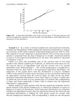
Example 4.5 A total of 9121 breast cancer cases were diagnosed in
Connecticut hospitals from 1935 to 1953. The Connecticut life table for white
females, 1939—1941, is used in calculation of the expected survival rate. Table
4.8 gives the observed and expected survival rates as well as the relative
survival rates. Figure 4.5a graphically shows these data: the survival curves for
the breast cancer patients and the general population. The relative survival
rates are plotted in Figure 4.5b. For this group of patients, the relative survival
rates, although increasing during 13 successive years, are less than 100%
throughout the 15 years of follow-up. During each of the 15 years, the
, -,     95
Table 4.8 Relative Survival Rates of Breast Cancer
Patients in Connecticut, 1935 1953
Survival Rates (%) Relative
Years after Survival Rate
Diagnosis Observed Expected (%)
0—1 82.9 97.2 85
1—2 83.3 97.1 86

2—3 85.9 96.9 89
3—4 86.8 96.7 90
4—5 89.2 96.6 92
5—6 90.0 96.4 93
6—7 89.9 96.4 93
7—8 91.6 96.2 95
8—9 92.0 96.1 96
9—10 92.7 96.1 96
10—11 92.9 95.9 97
11—12 94.0 95.8 98
12—13 94.1 95.3 99
13—14 91.5 95.3 96
14—15 90.6 94.9 95
Source: Cutler et al. (1957).
breast cancer patient mortality rate is greater than that of the general
population.
Other measures of describing survival experience of cancer patients are the
five-year survival rate and the corrected rate. The five-year survival rate is
simply the cumulative proportion surviving at the end of the fifth year. For
example, the five-year survival rate for the males with angina pectoris in
Example 4.4 is 0.5193. The five-year survival rate is no longer a measure of
treatment success for patients with many types of cancer since the survival of
cancer patients has improved considerably in the last few decades.
Berkson (1942) suggests using a corrected survival rate. This is the survival
rate if the disease under study alone is the cause of death. In most survival
studies, the proportion of patients surviving is usually determined without
considering the cause of death, which might be unrelated to the specific illness.
If p
A
denotes the survival rate when cancer alone is the cause of death, Berkson

proposes that
p
A
:
p
p

(4.3.3)
where p is the observed total survival rate in a group of cancer patients and p

is the survival rate for a group of the same age and gender in the general
96      
Figure 4.5 Survival rates of breast cancer patients in Connecticut, 1935—1953.
population. Rate p
A
may be computed at any time after the initiation of
follow-up; it provides a measure of the proportion of patients that escaped a
death from cancer up to that point. If a five-year survival rate is 0.5 and it is
corrected for noncancer deaths and if we find that five-year survival rate of the
general population is 0.9, the corrected survival rate is 0.5/0.9, or 0.56.
4.4 STANDARDIZED RATES AND RATIOS
Rates and ratios are often used in demography and epidemiology to describe
the occurrence of a health-related event. For example, the standardized
mortality (or morbidity) ratio (SMR) is frequently used in occupational
epidemiology as a measure of risk, and the standardized death rate is
commonly used in comparing mortality experiences of different populations or
the same population at different times.
The concept of the SMR is very similar to that of the relative survival rate
described above. It is defined as the ratio of the observed and the expected
number of death and can be expressed as

SMR :
observed number of deaths in study population
expected number of deaths in study population
;100 (4.4.1)
where the expected number of deaths is the sum of the expected deaths from
the same age, gender, and race groups in the general population. The
standardized morbidity ratio can similarly be calculated simply by replacing
the word deaths by disease cases in (4.4.1). If only new cases are of interest, we
call the ratio the standardized incidence ratio (SIR).
    97
Table 4.9 Population and Deaths of Sunny City and Happy City by Age
Sunny City Happy City
Age-Specific Age-Specific
Rates Rates
Age Population Deaths (per 1000) Population Deaths (per 1000)
:25 25,000 25 1.00 55,000 110 2.0
25—44 40,000 50 1.25 20,000 50 2.5
45—64 20,000 200 10.00 21,000 315 15.0
.65 15,000 1,200 80.00 4,000 650 162.5
Total 100,000 1,475 100,000 1,125
The standardized death rate is only one of the many rates used to describe
the health status of a population or to compare the health status of different
populations. If the populations are similar with respect to demographic
variables such as age, gender, or race, the crude rate, or ratio of the number of
persons to whom the event under study occurred to the total number of
persons in the population, can safely be used for comparison.
The level of the crude rate is affected by demographic characteristics of the
population for which the rate is computed. If populations have different
demographic compositions, a comparison of the crude rates may be mislead-
ing. As an example consider the two hypothetical populations, Sunny City and

Happy City, in Table 4.9. The crude death rate of Sunny City is 1000(1475/
100,000) or 14.7 per 1000. The crude death rate of Happy City is 1000(1125/
100,000), or 11.25 per 1000, which is lower than that of Sunny City even though
all age-specific rates in Happy City are higher. This is mainly because there is
a large proportion of older people in Sunny City. A crude death rate of a
population may be relatively high merely because the population has a high
proportion of older people; it may be relatively low because the population has
a high proportion of younger people. Thus, one should adjust the rate to
eliminate the effects of age, gender, or other differences. The procedure of
adjustment is called standardization and the rate obtained after standardization
is called the standardized rate.
The most frequently used methods for standardization are the direct method
and the indirect method.
Direct Method
In this method a standard population is selected. The distribution across the
groups with different values of the demographic characteristic (e.g., different
age groups) must be known. Let r

, , r
I
, where k is the number of groups,
be the specific rates of the different groups for the population under study. Let
p

, , p
I
be the proportions of people in the k groups for the standard
population. The direct standardized rate is obtained by multiplying the specific
98      
rates r

G
by p
G
in each group. The formula for the direct standardized rate is
R

:
I

G
r
G
p
G
(4.3.2)
As an example, consider the data in Table 4.9. If we choose a standard
population whose distribution is shown in the second column of Table 4.10,
the direct standardized death rate for Sunny City and Happy City is, respect-
ively, 9.37 and 17.84 per 1000. These standardized rates are more reliable than
the crude rates for comparison purposes.
Indirect Method
If the specific rates r
G
of the population being studied are unknown, the direct
method cannot be applied. In this case, it is possible to standardize the rate by
an indirect method if the following are available:
1. The number of persons to whom the event being studied occurred (D) in
the population. For example, if the death rate is being standardized, D is
the number of deaths.
2. The distribution across the various groups for the population being

studied, denoted by n

, , n
I
.
3. The specific rates of the selected standard population, denoted by
s

, , s
I
.
4. The crude rate of the standard population, denoted by r.
The formula for indirect standardization is
R

:
D

I
G
n
G
s
G
r (4.3.3)
The summation in (4.3.3) is the expected number of persons to whom the event
occurred on the basis of the specific rates of the standard population. Thus, the
indirect method adjusts the crude rate of the standard population by the ratio
of the observed to expected number of persons to whom the event occurred in
the population under study.

Table 4.11 represents an example for the death rate in the states of
Oklahoma and Arizona in 1960 (data are from Grove and Hetzel, 1963). The
U.S. population in 1960 is used as the standard population. The crude death
rate of Oklahoma (9.7 per thousand) is higher than that of Arizona (7.8 per
thousand). However, the indirect standardized rates show a reverse relation-
ship (8.6 for Oklahoma and 9.6 for Arizona). This, again, is because of the
differences in age distribution. There is a higher proportion of people below the
age of 25 in Arizona and a higher proportion of people above the age of 54 in
Oklahoma.
    99
Table 4.10 Standardized Death Rates by Direct Method for Sunny City and Happy City
Sunny City Happy City
Age-Specific Age-Standardized Age-Specific Age-Standardized
Standard Proportion, Death Rates, Death Rates, Death Rates, Death Rates,
Age Population p
G
r
G
p
G
r
G
r
G
p
G
r
G
:25 420,000 0.42 1.00 0.42 2.00.84
25—44 280,000 0.28 1.25 0.35 2.5 0.70

45—64 220,000 0.22 10.00 2.20 15.0 3.30
.65 80,000 0.08 80.00 6.40 162.5 13.00
Total 1,000,000 9.37 17.84
(R

)(R

)
100
Table 4.11 Standardized Death Rates by Indirect Method for Oklahoma and Arizona, 1960
Oklahoma Arizona
Standard Population
(U.S. Population, 1960) Expected Expected
Age-Specific Death Rates, Population, Deaths, Population, Deaths,
Age s
G
n
G
n
G
s
G
n
G
n
G
s
G
:10.0270 49,103 1,325.78 34,599 934.17
1—4 0.0011 193,644 213.01 132,367 145.60

5—14 0.0005 454,972 227.49 285,830 142.92
15—24 0.0011 329,230 362.15 186,789 205.47
25—34 0.0015 279,327 418.99 169,873 254.81
35—44 0.0030 287,994 863.98 173,029 519.09
45—54 0.0076 269,147 2,045.52 136,573 1,037.95
55—64 0.0174 216,036 3,759.03 92,871 1,615.96
65—74 0.0382 157,385 6,012.11 63,634 2,430.82
75—84 0.0875 74,848 6,549.20 22,499 1,968.66
85; 0.1986 16,598 3,296.36 4,092 812.67
Total 2,328,284 25,074 1,302,161 10,068
Crude rates 9.5 9.7 7.8
(per thousand)
Observed deaths 22,584 10,157
Expected deaths? 25,074 10,068
Standardized rate

22,584
25,074

9.5 : 8.6

10,157
10,068

9.5 : 9.6
(per thousand)
Source: Data from Grove and Hetzel (1963).
?  n
G
s

G
.
101
Results for the adjusted rates depend on the standard population selected.
Hence, this selection should be done carefully. When discussing death rate by
age, Shryock et al. (1971) suggest that a population with similar age distribu-
tion to the various populations under study be selected as a standard. If the
death rate of two populations is being compared, it is best to use the average
of the two distributions as a standard.
It should be remembered that specific rates are still the most accurate and
essential indicators of the variations among populations. No matter which
method is used, standardized rates are meaningful only when compared with
similarly computed rates. Kitagawa (1964) also criticizes the standardized rate
because if the specific rates vary in different ways between the two populations
being compared, standardization will not indicate the differences and some-
times will even mask the differences. Nevertheless, if the specific rates are not
available, if a single rate for a population is desired, or if the demographic
composition of the population being compared is different, the standardized
rate is useful.
Bibliographical Remarks
Kaplan and Meier’s (1958) PL method is the most commonly used technique
for estimating the survivorship function for samples of small and moderate size.
However, with the aid of a computer, it is not difficult to use the method for
large sample sizes.
Berkson (1942), Berkson and Gage (1950), Cutler and Ederer (1958), and
Gehan (1969) have written classic reports on life-table analysis. Peto et al.
(1976) published an excellent review of some statistical methods related to
clinical trials. The term life-table analysis that they use includes the PL method.
Other references on life tables are, for example, Armitage (1971), Shryock et al.
(1971), Kuzma (1967), Chiang (1968), Gross and Clark (1975), and Elandt-

Johnson and Johnson (1980).
Relative survival rates and corrected survival rates have been used by Cutler
and co-workers in a series of survival studies on cancer patients in Connecticut
in the 1950s and 1960s (Cutler et al., 1957, 1959, 1960a, b, 1967; Ederer et al.,
1961). Discussions of SMR, standardized rates, and related topics can be found
in many standard epidemiology textbooks: for example, Mausner and Kramer
(1985), Kahn (1983), Kelsey et al. (1986), Shryock et al. (1971), Chiang (1961),
and Mantel and Stark (1968).
EXERCISES
4.1 Consider the survival time of the 30 melanoma patients in Table 3.1.
(a) Compute and plot the PL estimates of the survivorship functions
S (t) of the two treatment groups and check your results with Table
3.2 and Figure 3.1.
102      
Exercise Table 4.1
Number
Time from Number Lost Withdrawn Number Number
Diagnosis to Follow-up, Alive, Dying, Entering,
(yr) l
G
w
G
d
G
n

G
0—5 18 0 731 949
5—10 16 0 52 200
10—15 8 67 14 132

15—20 0 33 10 43
(b) Compute the variance of S (t) for every uncensored observation.
(c) Estimate the median survival times of the two groups.
4.2 Do the same as in Exercise 4.1 for the remission durations of the two
treatment groups in Table 3.1.
4.3 Compute and plot the PL estimates of the tumor-free time distributions
for the saturated fat and unsaturated fat diet groups in Table 3.4.
Compare your results with Figure 3.4.
4.4 Consider the remission data of 42 patients with acute leukemia in
Example 3.3.
(a) Compute and plot the PL estimates of S(t) at every time to relapse
for the 6-MP and placebo groups.
(b) Compute the variances of S (10) in the 6-MP group and of S (3) in
the placebo group.
(c) Estimate the median remission times of the two treatment groups.
4.5 (a) Compute the survival time for each patient in Exercise Table 3.1.
(b) Estimate and plot the overall survivorship function using the PL
method. What is the median survival time?
(c) Divide the patients into two groups by gender. Compute and plot
the PL estimates of the survivorship functions for each group. What
is the median survival time for each?
4.6 Consider the skin test results in Exercise Table 3.1. For each of the five
skin tests:
(a) Divide patients into two groups according to whether they had a
positive reaction. Measurements less than 10;10 (5;5 for mumps)
are considered negative.
(b) Estimate and plot the survivorship functions of the two groups.
(c) Can you tell from the plots if any skin tests might predict survival
time?
4.7 Consider the data of patients with cancer of the ovary diagnosed in

Connecticut from 1935 to 1944 (Cutler et al. 1960b). Exercise Table 4.1
 103
Exercise Table 4.2 Survival Data of Female Patients with Angina Pectoris
Year After Number Entering Number Lost to
Diagnosis Interval Follow-up Number Dying
0—1 555 0 82
1—2 473 8 30
2—3 435 8 27
3—4 400 7 22
4—5 371 7 26
5—6 338 28 25
6—7 285 31 20
7—8 234 32 11
8—9 191 24 14
9—10 153 27 13
10—11 113 22 5
11—12 86 23 5
12—13 58 18 5
13—14 35 9 2
14—15 24 7 3
15; 14 11 3
Source: R. L. Parker et al., JAMA, 131(2),95—100 (1946). Copyright 1946. American Medical
Association.
reproduces the data in life-table format. Provide a life-table like Table
4.5. What do you find out?
4.8 Do a complete life-table analysis for the two sets of data given in Table
3.5. Plot the three survival functions.
4.9 Do a complete life-table analysis of the data given in Exercise Table 4.2.
Plot the three survival functions.
4.10 Consider the survival times of the melanoma patients in Exercise Table

3.4. Do a complete life-table analysis of the survival time. Plot the three
survival functions.
4.11 Consider the data given in Exercise Table 4.3. Compute the direct
standardized death rate for the states of Oklahoma and Montana using
the U.S. population of 1960 as the standard.
4.12 Given the population of Japan and Chile (Exercise Table 4.4), compute
the indirect standardized death rate for the two countries using the U.S.
death rate of 1960 in Table 4.11 as the standard.
104      
Exercise Table 4.3
Oklahoma Average Montana Average
Death Rate Death Rate
U.S. Population, Proportion, (per 1000)(per 1000)
Age 1960 (thousands) p
G
r
G
r
G
:1 4,112 0.023 25.525.8
1—4 16,209 0.091 1.2 1.2
5—14 35,465 0.198 0.5 0.5
15—24 24,020 0.134 1.2 1.6
25—34 22,818 0.127 1.6 1.8
35—44 24,081 0.134 2.9 3.1
45—54 20,486 0.114 6.9 7.5
55—64 15,572 0.087 14.8 16.3
65—74 10,997 0.061 32.4 37.3
75—84 4,634 0.026 79.0 87.3
85; 929 0.005 190.4 202.8

Total 179,323 1.000
Source: Grove and Hetzel (1963).
Exercise Table 4.4
Population
(thousands)
Age Japan Chile
:1 1,577 228
1—4 6,268 876
5—14 20,223 1,817
15—24 17,627 1,323
25—34 15,727 1,034
35—44 11,057 779
45—54 9,018 603
55—64 6,573 395
65—74 3,724 212
75—84 1,438 83
-85 188 22
———— ———
Total 93,419 7,374
Observed deaths 706,599 95,486
Source: Shryock et al. (1971).
 105
CHAPTER 5
Nonparametric Methods for
Comparing Survival Distributions
The problem of comparing survival distributions arises often in biomedical
research. A laboratory researcher may want to compare the tumor-free times
of two or more groups of rats exposed to carcinogens. A diabetologist may
wish to compare the retinopathy-free times of two groups of diabetic patients.
A clinical oncologist may be interested in comparing the ability of two or more

treatments to prolong life or maintain health. Almost invariably, the disease-
free or survival times of the different groups vary. These differences can be
illustrated by drawing graphs of the estimated survivorship functions, but that
gives only a rough idea of the difference between the distributions. It does not
reveal whether the differences are significant or merely chance variations. A
statistical test is necessary.
In Section 5.1 we introduce five nonparametric tests that can be used for
data with and without censored observations. Section 5.2 is devoted to the
Mantel—Haenszel test, which is particularly useful in stratified analysis, a
method commonly used to take account of possible confounding variables. In
Section 5.3 we discuss the problem of comparing three or more survival
distributions with or without censoring.
5.1 COMPARISON OF TWO SURVIVAL DISTRIBUTIONS
Suppose that there are n

and n

patients who receive treatments 1 and 2,
respectively. Let x

, , x
P

be the r

failure observations and x
>
P

>

, ,x
>
L

the
n

9 r

censored observations in group 1. In group 2, let y

, , y
P

be the r

failure observations and y
>
P

>
, ,y
>
L

the n

9 r

censored observations. That

is, at the end of the study n

9 r

patients who received treatment 1 and
n

9 r

patients who received treatment 2 are still alive. Suppose that the
observations in group 1 are samples from a distribution with survivorship
function S

(t) and the observations in group 2 are samples from a distribution
106
with survivorship function S

(t). Then null hypothesis to consider is
H

: S

(t) : S

(t) (treatments 1 and 2 are equally effective)
against the alternative
H

: S


(t) 9S

(t) (treatment 1 more effective than 2)
or
H

: S

(t) :S

(t) (treatment 2 more effective than 1)
or
H

: S

(t) "S

(t) (treatments 1 and 2 not equally effective)
When there are no censored observations, standard nonparametric tests can
be used to compare two survival distributions. For example, the Wilcoxon
(1945) test or the Mann—Whitney (1947) U-test can test the equality of two
independent populations, and the sign test can be used for paired (or depend-
ent) samples (Marascuilo and McSweeney, 1977). In the following we introduce
five nonparametric tests: Gehan’s generalized Wilcoxon test (Gehan, 1965a,b),
the Cox—Mantel test (Cox 1959, 1972; Mantel, 1966), the logrank test (Peto
and Peto, 1972), Peto and Peto’s generalized Wilcoxon test (1972), and Cox’s
F-test (1964). All the tests are designed to handle censored data; data without
censored observations can be considered a special case.
5.1.1 Gehan’s Generalized Wilcoxon Test

In Gehan’s generalized Wilcoxon test every observation x
G
or x
>
G
in group 1 is
compared with every observation y
H
or y
>
H
in group 2 and a score U
GH
is given
to the result of every comparison. For the purpose of illustration, let us assume
that the alternative hypothesis is H

: S

(t) 9 S

(t), that is, treatment 1 is more
effective than treatment 2.
Define
U
GH
:

;1ifx
G

9 y
H
or x
>
G
. y
H
0ifx
G
: y
H
or x
>
G
: y
H
or y
>
H
: x
G
or (x
>
G
, y
>
H
)
91ifx
G

: y
H
or x
G
- y
>
H
and calculate the test statistic
W :
L


G
L


H
U
GH
(5.1.1)
where the sum is over all n

n

comparisons. Hence, there is a contribution to
     107
the test statistic W for every comparison where both observations are failures
(except for ties) and for every comparison where a censored observation is
equal to or larger than a failure. The calculation of W is laborious when n


and n

are large. Mantel (1967) shows that it can be calculated in an alternative
way by assigning a score to each observation based on its relative ranking. In
Gehan’s computation each observation in sample 1 is compared with each in
sample 2. If the two samples are combined into a single pooled sample of
n

; n

observations, it is the same as comparing each observation with the
remaining n

; n

9 1. Let U
G
, i : 1, , n

; n

, be the number of remaining
n

; n

9 1 observations that the ith is definitely greater than minus the
number that it is definitely less than. The n

; n


U
G
’s define a finite population
with mean 0 and it is true that Gehan’s
W :
L


G
U
G
(5.1.2)
where summation is over the U
G
of sample 1 only. From either (5.1.1) or (5.1.2),
it is clear that W would be a large positive number if H

is true. Mantel also
suggests that the permutational variance of W be used instead of the more
complicated variance formula derived by Gehan. The permutational distribu-
tion of W can be obtained by considering all

n

; n

n



:
(n

; n

)!
n

! n

!
ways of selecting n

of the U
G
at random. The test statistic W under H

can be
considered approximately normally distributed with mean 0 and variance
Var(W ) :
n

n

L

>L


G

U

G
(n

; n

)(n

; n

9 1)
(5.1.3)
Since W is discrete, an appropriate continuity correction of 1 is ordinarily used
when there are neither ties nor censored observations. Otherwise, a continuity
correction of 0.5 would probably be appropriate.
Since W has an asymptotically normal distribution with mean zero and
variance in (5.1.3), Z : W/
(
Var(W ) has standard normal distribution. The
rejection regions are Z 9Z
?
for H

, and Z :9Z
?
for H

, and "Z"9Z
?

for
H

where P(Z 9 Z
?
" H

) : .
 n! is read n factorial: n! : n(n 9 1)(n 9 2) %3.2.1.
 This is called the permutational variance because it is obtained by considering the per mutational
distribution of all (n

; n

)!/n

! n

! W ’s
108      
The number U
G
can be computed in two stages. For each observation, the
first stage yields, unity plus the number of remaining observations that it is
definitely larger than, that is, R
G
. The second stage yields R
G
, which is unity
plus the number of remaining observations that the particular observation is

definitely less than. Then U
G
: R
G
9 R
G
. The computations of R
G
and R
G
can
be accomplished systematically in steps, as illustrated in the following hypo-
thetical example.
Example 5.1 Ten female patients with breast cancer are randomized to
receive either CMF (cyclic administration of cyclophosphamide, methatrexate,
and fluorouracil) or no treatment after a radical mastectomy. At the end of two
years, the following times to relapse (or remission times) in months are
recorded:
CMF (group 1): 23, 16;,18;,20;,24;
Control (group 2): 15, 18, 19, 19, 20
The null hypothesis and the alternatives are
H

: S

: S

(the two treatments are equally effective)
H


: S

9 S

(CMF more efficient than no treatment)
The computations of R
G
, R
G
, and U
G
are given in Table 5.1. Thus,
W : 1 ; 2 ; 5 ; 4 ; 6 : 18, Var(W ) : (5)(5)(208)/[(10)(9)] : 57.78, and
Z : 18/(57.78: 2.368. Suppose that the significance level used is : 0.05,
Z

: 1.64; then the Z value computed is in the rejection region. Therefore,
we reject H

at 0.05 level and conclude that the data show that CMF is more
effective than no treatment. In fact, the approximate p value corresponding to
Z : 2.368 is 0.009.
Note that the sum of all n

; n

U
G
’s equals zero. This fact can be used to
check the computation.

5.1.2 Cox Mantel Test
Let t

: ···:t
I
be the distinct failure times in the two groups together and
m
G
be the number of failure times equal to t
G
, or the multiplicity of t
G
, so that
I

G
m
G
: r

; r

(5.1.4)
Further, let R(t) be the set of people still exposed to risk of failure at time
t, whose failure or censoring times are at least t. Here R(t) is called the risk set
at time t. Let n
R
and n
R
be the number of patients in R(t) that belong to

     109
Table 5.1 Mantel’s Procedure of Calculating U
i
for Gehan’s Generalized Wilcoxon Test
Observations of Two
Samples in Ascending
Order 15 16> 18 18> 19 19 20 20> 23 24>
Computation of R
G
Step 1. Rank from left to
right, omitting
censored
observations 1 2 3 4 5 6
Step 2. Assign next-higher
rank to censored
observations 2 3 6 7
Step 3. Reduce the rank
of tied observations
to the lower rank
for the value 3
Step 4. R
G
12 23 335 6 67
Computation of R
G
Step 5. Rank from right
to left 10 9 8 7 6 5 4 3 2 1
Step 6. Reduce the rank of
tied observations to
the lowest rank for

the value 5
Step 7. Reduce the rank
of censored
observations to 1 1 1 1 1
Step 8. R
G
10181554121
U
G
: R
G
9 R
G
991? 962? 92 921 5? 4? 6?
? From group 1.
treatment groups 1 and 2, respectively. The total number of observations,
failure or censored in R(t
G
), is r
G
: n
R
; n
R
. Define
U : r

9
I


G
m
G
A
G
(5.1.5)
I :
I

G
m
G
(r
G
9 m
G
)
r
G
9 1
A
G
(1 9 A
G
) (5.1.6)
where r
G
is the number of observations, failure or censored, in R(t
G
) and A

G
110      
Table 5.2 Computations of Cox Mantel Test
Number in Risk Set of:
Distinct Sample 1 Sample 2
Failure Time, t
G
m
G
n
R
n
R
r
G
A
G
15 1 5 5 10 0.5
18 1 4 4 8 0.5
19 2 3 3 6 0.5
20 1 3 1 4 0.25
23 1 2 0 2 0
is the proportion of r
G
that belong to group 2. An asymptotic two-sample test
is thus obtained by treating the statistic C : U/(I as a standard normal
variate under the null hypothesis (Cox, 1972). The following example illustrates
the procedure.
Example 5.2 Consider the remission data and the hypotheses in Example
5.1. There are k : 5 distinct failure times in the two groups, r


: 1 and r

: 5.
To perform the Cox—Mantel test, Table 5.2 is prepared for convenience:
U : 59 (0.5 ; 0.5 ; 2 ;0.5 ; 0.25)
: 5 9 2.25
: 2.75
I :
1;9
9
(0.5;0.5) ;
1;7
7
(0.5;0.5) ;
2;4
5
(0.5;0.5) ;
1;3
3
(0.25;0.75)
: 0.25 ; 0.25 ; 0.4 ; 0.1875
: 1.0875
Therefore, C : 2.75/(1.0875 : 2.6379 Z

: 1.64 and we reject H

at 0.05
level and reach the same conclusion as in Example 5.1. The p value correspond-
ing to Z : 2.637 is approximately 0.004.

5.1.3 Logrank Test
Mantel’s (1966) generalization of the Savage (1956) test, often referred to as the
logrank test (Peto and Peto, 1972), is based on a set of scores w
G
assigned to
the observations. The scores are functions of the logarithm of the survival
     111
function. Altshuler (1970) estimates the log survival function at t
G
using
9e(t
G
) :9 
j-t
G
m
H
r
H
(5.1.7)
where m
H
and r
H
are as defined in Section 5.1.2. The scores suggested by Peto
and Peto are w
G
: 1 9 e(t
G
) for an uncensored observation t

G
and 9e(T ) for
an observation censored at T. In practice, for a censored observation t
>
G
,
w
G
:9e(t
H
), where t
H
is the largest uncensored observation that t
H
- t
>
G
.
Thus, the larger the uncensored observation, the smaller its score. Censored
observations receive negative scores. The w scores sum identically to zero for
the two groups together. The logrank test is based on the sum S of the w scores
of the two groups. The permutational variance of S is given by
Var(S) :
n

n


L


>L

G
w

G
(n

; n

)(n

; n

9 1)
(5.1.8)
which can be rewritten as
V :

I

H
m
H
(r
H
9 m
H
)
r

H

n

n

(n

; n

)(n

; n

9 1)
(5.1.9)
The test statistic L : S/(Var(S ) has an asymptotically standard normal
distribution under the null hypothesis. If S is obtained from group 1, the critical
region is L : 9Z
?
, and if S is obtained from group 2, the critical region is
L 9 Z
?
, where  is the significance level for testing H

: S

: S

against

H

: S

9 S

. The following example illustrates the computational procedures.
Example 5.3 Consider the data and hypotheses in Example 5.1. The test
statistic of the logrank test can be computed by tabulating m
G
, r
G
, m
G
/r
G
,
and e(t
G
) as in Table 5.3. Since every observation in the two samples, censored
or not, is assigned a score, it is convenient to list them in column 1. Columns
2 to 5 pertain only to the failure times; e(t
G
) is the cumulative value of m
G
/r
G
,
Altshuler’s (1970) estimate of the logarithm of the survivorship function
multipled by 91. For example, at t

G
: 18, e(t
G
) : 0.100 ; 0.125 : 0.225; at
t
G
: 19, e(t
G
) : 0.225 ; 0.333 : 0.558. The last column, w
G
, gives the score for
every observation. For an uncensored observation w
G
: 1 9 e(t
G
), for example,
at t
G
: 18, w
G
: 1 9 0.225 : 0.775. Since e(t
G
) is an estimate of a function of
the survivorship function, which we assume to be constant between two
consecutive failures, e(t
>
G
) is equal to e(t
H
) for t

H
-t
>
G
. Thus w
G
for censored
observations t
>
G
equals 9e(t
H
), where t
H
- t
>
G
. For example, w
G
for 16> is
9e(15), or 90.100, and that for 18> is 9e(18), or 90.225. Tied observations
like the two 19’s receive the same score: 0.442. The 10 scores w
G
sum to zero,
which can be used to check the computation.
112      
Table 5.3 Computations of Logrank Test
Remission Times
in Both Samples,
t

G
m
G
r
G
m
G
/r
G
e(t
G
) w
G
15 1 10 0.100 0.100 0.900?
16; —— — — 90.100
18 1 8 0.125 0.225 0.775?
18; —— — — 90.225
19 2 6 0.333 0.558 0.442?
20 1 4 0.250 0.808 0.192?
20; —— — — 90.808
23 1 2 0.500 1.308 90.308
24; —— — — 91.308
? From sample 2.
The statistic S : 0.900 ; 0.775 ; 0.442 ; 0.442 ; 0.192 : 2.751. The vari-
ance of S, computed by (5.8) is 1.210. Hence, the test statistic L :2.751/
(1.210 : 2.5 and the p value is approximately 0.0064, data showing that CMF
treatment is superior. The logrank statistic S can be shown to equal the sum
of the failures observed minus the conditional failures expected computed at
each failure time, or simply the difference between the observed and expected
failures in one of the groups. A similar version of the logrank test is a

chi-square test which compares the observed number of failures to the expected
number of failures under the hypothesis. Let O

and O

be the observed
numbers and E

and E

the expected numbers of death in the two treatment
groups. The test statistic
X:
(O

9 E

)
E

;
(O

9 E

)
E

(5.1.10)
has approximately the chi-square distribution with 1 degree of freedom. A large

X value (e.g., .X


) would lead to the rejection of the null hypothesis in
favor of the alternative that the two treatments are not equally effective
( : 0.05).
To compute E

and E

, we arrange all the uncensored observations in
ascending order and compute the deaths expected at each uncensored time and
sum them. The number of deaths expected at an uncensored time is obtained
by multiplying the deaths observed at that time by the proportion of patients
exposed to risk in the treatment group. Let d

be the number of deaths at time
t and n
R
and n
R
be the numbers of patients still exposed to risk of dying at
time up to t in the two treatment groups. The deaths expected for groups 1
     113
Table 5.4 Computation of E
1
of Logrank Test
Relapse time, td
R
n

R
n
R
e
R
e
R
15 1 5 5 0.5 0.5
18 1 4 4 0.5 0.5
19 2 3 3 1.0 1.0
20 1 3 1 0.75 0.25
23 1 2 0 1.0 0
Total 3.75 2.25
and 2 at time t are
e
R
:
n
R
n
R
; n
R
;d
R
e
R
:
n
R

n
R
; n
R
;d
R
(5.1.11)
Then the total numbers of deaths expected in the two groups are
E

: 
 R
e
R
E

: 
 R
e
R
In practice, we only need to compute the total number of deaths expected
in one of the two groups, for example, E

, since E

is the total observed number
of deaths minus E

. The following example illustrates the calculation pro-
cedure.

Example 5.4 Let us use the hypothetical data in Example 5.1 again. The
remission times in months are:
CMF (group 1): 23, 16
;
,18
;
,20
;
,24
;
Control (group 2): 15, 18, 19, 19, 20.
Consider the following null and alternative hypotheses:
H

: S

: S

(the two treatments are equally effective)
H

: S

" S

(the two treatments are not equally effective)
Table 5.4 gives the calculation of E

. For example, at t : 18, four patients
in group 1 and four in group 2 are still exposed to the risk of relapse, and there

is one relapse. Thus, d
R
: 1, n
R
: n
R
: 4, and e
R
: 0.5.
The total number of relapses expected is E

: 3.75. Since there are a total of
six deaths (O

: 1, O

: 5) in the two groups, E

: 69 3.75 : 2.25. Using
114      
(5.1.10), we have
X:
(1 9 3.75)
3.75
;
(5 9 2.25)
2.25
: 5.378
Using Table C-2, the p value corresponding to this X value is less 0.05
(p < 0.02). Therefore, we reach the same conclusion: that there is a significant

difference in remission duration between the CMF and control groups.
Computer software is available to perform a number of two-sample tests
with censored observations. For example, SAS, SPSS, and BMDP provide
procedures for the logrank and Cox—Mantel tests. We use the remission time
of the 10 breast cancer patients in Example 5.1 to illustrate the use of these
software packages. To compare the two groups, we create the following three
variables: t, remission time; CENS: 0ift is censored and 1 otherwise; and
TREAT : 1 if receiving CMF and :2 if no treatment. Assume that the data
have been saved in ‘‘C:!D5d1.DAT’’ as a text file, which contains three
columns, separated by a space (t is in the first column, CENS the second
column, and TREAT the third column), and the data in each row are for the
same patient. The following SAS code can be used to perform the logrank test.
data w1;
infile ‘c:!d5d1.dat’ missover;
input t cens treat;
run;
proc lifetest data: w1;
time t*cens(0);
strata treat;
run;
If BMDP procedure 1L is used, the following code can be used to perform
the Cox—Mantel test.
/input file : ‘c:!d5d1.dat’ .
variables : 3.
format : free.
/variable names : t, cens, treat.
/form time : t.
status : cens.
response : 1.
/group codes(treat) : 1, 2.

Names(treat) : treated, control.
/estimate method : product.
Group : treat.
Stat : mantel.
/end
     115
If procedure KM in SPSS is used, the following code can be used to perform
the Cox—Mantel test.
data list file : ‘c:!d5d1.dat’ free
/ t cens treat.
km t by treat
/status : cens event (1)
/test : logrank.
These codes can be modified to perform tests comparing more than two groups
simply by replacing TREAT in the codes with the group variable defined.
5.1.4 Peto and Peto’s Generalized Wilcoxon Test
Another generalization of Wilcoxon’s two-sample rank sum test is described by
Peto and Peto (1972). Similar to the logrank test, this test assigns a score to
every observation. For an uncensored observation t, the score is u
G
:
S (t;) ; S (t9) 9 1, and for an observation censored at T, the score is
u
G
: S (T ) 9 1, where S is the Kaplan—Meier estimate of the survival function.
If we use the notation of Section 5.1.2, the score for an uncensored observation
t
G
is u
G

: S (t
G
) ; S (t
G\
) 9 1 and S (t

) : 0 and that for a censored observa-
tion is t
>
H
is u
H
: S (t
G
) 9 1, where t
G
- t
>
H
. These generalized Wilcoxon scores
sum to zero. The test procedure after the scores are assigned is the same as for
the logrank test. The following example illustrates the computational pro-
cedures.
Example 5.5 Using the same data and hypotheses as in Example 5.1, the
calculations of the scores u
G
for Peto and Peto’s generalized Wilcoxon test are
given in Table 5.5. Using the scores of group 1, we obtain
S :90.1009 0.2129 0.605 9 0.408 9 0.803 :92.128
Var(S) : (5)(5)

(0.9);% ; (90.803)
10 ;9
: 0.765
Thus, Z :92.128/(0.765 :92.433: 9Z

:91.64. We reject H

at the
0.05 level and reach the same conclusion as in the last three examples: that the
data show that CMB is more effective than no treatment.
5.1.5 Cox’s F-test
Cox’s F-test (Cox, 1964) is based on ordered scores from the exponential
distribution. It is for singly censored or complete samples; it is not applicable
to progressively censored data. The procedure is as follows:
116      
Table 5.5 Computations of Peto and Peto’s
Generalized Wilcoxon Test
t
G
S (t) u
G
15 0.900 1; 0.900 9 1 : 0.900
16; — 0.9009 1 :90.100?
18 0.788 0.900 ; 0.788 9 1 : 0.688
18; — 0.7889 1 :90.212?
19 0.657 0.788 ; 0.657 9 1 : 0.445
19 0.526 0.526 ; 0.657 9 1 : 0.183
20 0.395 0.395 ; 0.526 9 1 :90.079
20; — 0.3959 1 :90.605?
23 0.197 0.197 ; 0.395 9 1 :904.08?

24; — 0.1979 1 :90.803?
? Group 1.
1. Rank the observations in the combined sample.
2. Replace the ranks by the corresponding expected order statistics in
sampling the unit exponential distribution [ f (t) : e\R]. Denote by t
PL
the
expected value of the rth observation in increasing order of magnitude,
t
PL
:
1
n
; % ;
1
n 9 r ; 1
r : 1, , n (5.1.12)
where n is the total number of observations in the two samples. In
particular,
t
L
:
1
n
t
L
:
1
n
;

1
n 9 1
$
t
LL
:
1
n
;
1
n 9 1
; %; 1
(5.1.13)
For n not too large, they can easily be computed by using tables of
reciprocals. When two or more observations are tied, the average of the
scores is used.
3. For data without censored observations, the entire set of n observations
is replaced by the set of scores +t
PL
, so obtained. The sample mean scores
denoted by t

and t

of the two samples with n

, n

observations are then
computed. The ratio t


/t

has been shown to follow an F distribution
with (2n

,2n

) degrees of freedom. Critical regions for testing H

: S

: S

     117
against H

(S

9 S

), H

(S

: S

), and H

(S


"S

) are, respectively,
t

/t

9 F
L

L

?
, t

/t

: F
L

L

\?
, and t

/t

9 F
L


L

?
or t

/
t

:F
L

L

\?
.
4. The calculation of F is slightly different for singly censored data. Let r

and r

be the number of failures and n

9 r

and n

9 r

the number of
censored observations in the two samples. Then there are p : r


; r

failures in the combined sample and n 9 p censored observations. Cox
(1964) suggests using the scores t
L
, , t
NL
as before for the failures and
t
N>L
for all censored observations. The mean score, for example, for the
first group is
t

:
r

t


; (n

9 r

)t
N>L
r

(5.1.14)

where t


is the mean score of the failures. The mean score for the second
group is calculated in a similar way. The F-statistic t

/t

, has an
approximate F-distribution with (2r

,2r

) degrees of freedom.
This test is for the hypothesis that the two samples are from populations
with equal means. It can also determine if the second population mean is k
times the first population mean, for a given k, by dividing the observations in
the second sample by k before ranking and applying the test. The set of all
values k not rejected in such a significance test forms a confidence interval. The
following example illustrates the computation.
Example 5.6 In an experiment comparing two treatments (A and B) for
solid tumor, suppose that the question is whether treatment B is better than
treatment A. Six mice are assigned to treatment A and six to treatment B. The
experiment is terminated after 30 days. The following survival times in days are
recorded. Our null and alternative hypotheses are H

: S

: S

and
H

: S

: S

.
Treatment A: 8, 8, 10, 12, 12, 13
Treatment B: 9, 12, 15, 20, 30
;
,30
;
That is, all the mice receiving treatment A die within 13 days and two mice
receiving treatment B are still alive at the end of the study. Do the data provide
sufficient evidence that treatment B is more effective than treatment A?
To compute the test statistic, it is convenient to set up a table like Table 5.6.
The first column lists all the observations in the two samples. The second
column contains the ordered exponential scores t
PL
. In this case, n

: 6, n

: 6,
n : 12, r

: 6, and r

: 4. The scores are computed following (5.1.12) and

(5.1.13). For example, t
PL
for t
G
: 10 is equal to 1/12 ; 1/11 ; 1/10 ; 1/9
or simply the previous t
PL
plus 1/9, that is, 0.274 ; 1/9 : 0.385. The
tied observations receive an average score: for example, for t
G
: 12,
118      