a guide to microsoft excel 2002 for scientists and engineers phần 10 ppt

286
A
Guide to
Microsoft Excel
2002
for
Scientists and Engineers
Correlation
0.97
Figure
14.8
(a)
On Sheet6 of
CHAPl4.XLS,
enter the text values shown
in
columns A:G of Figure
14.8.
For now, ignore columns
I:K.
Enter the values shown in
A4:C9.
(b) Enter the formula
=B4-C4
in
D4
and copy it down to
row
9.
(c) The formulas
in

column
G
are:
G3:
=AVERAGE(W:DS)
Computes
7
G4:
=COUNT(ALL:AS)
Computes
n
G5:
=DEVSQ(DI:DS)
Computes
C(d,
-iV
G6:
=SQRT(GS/(G4-1))
Computes
sd
G7:
=G3*SQRT(G4)/G6
Compute
t(experimental)
G8:
0.05
The required a-value
G9:
=TINV(G8, G4-1)
Computes

t(critical)
G10:
=IF(G7<GS,"same","not
same")
(314:
=TTEST(B4:B9,C4:C9,2,1)
Computes thep-value
We
are led to the conclusion that the
two
methods give the same
mean (with an a-value
of
0.05)
since (i)
t(experirnental)
is
less than
t(critical)
and (ii) thep-value computed by TTEST
is
greater than
the alpha value or
0.05.
To
round off this exercise, we use the
t-TEST: Paired Two Sample
for
Means
tool from the Data Analysis tool. This

is
left as an
exercise for the reader. Note that you should set the
Hypothesized
mean dzfference
to
0
and the
alpha
value to
0.05
when completing
the tool's dialog box. The results are shown in the figure.
As
expected, the results agree with our own calculations. The
t(experimental)
values in
G9
and
J
1
5
are the same,
as
are the
p-
values in
G14
and
J

14.
These serve
as
useful checks but recall that
the results from the tool are static whereas our calculations will be
updated if new experimental array values are entered.
Statistics for Experimenters
287
Exercise
7:
Comparing
Repeated
Measurements
8
When the two data sets are
of
equal size, this reduces to
s
P
=J($
+s3/2
.
In the previous exercise each sample was measured once by each
of
two
techniques. In this exercise the same sample
is
measured
repeatedly by
two

techniques. Our task is the same, to determine
if the mean
of
the
two
sets of measurements is the same. Once
again, we have
two
statistical methods we could use: the t and the
p
methods. For the former we compute a pooled standard deviation
using the formula$:
s=
n, +n,
-1
n, +n2
-2
P
from this we compute t(experimentaZ) and compare it with
t(criticaZ). The experimental t-value is found using:
For thep method we will again use the Microsoft Excel functions
TDIST
or
TTEST to find a probability value which we will
compare to the required a-value. We will also use the Data
Analysis tool t-Test: Two Sample Assuming Equal Variance to
check our results.
(a) On Sheet7 of CHAP 14.XLS enter the text shown in
A
1

:
D
19 of
Figure 14.9. Enter the experimental values
in
columns
A
and
B. Select A4:B 19 and use the InsertlEame command to name
Al:A19 as
A
and B1:B19 as
B.
This will allow the worksheet
to be used with up to
15
data points.
179.729 179.66
0.1025
Pooled Variance
0.01 1
179.731
179.749
179.705
179.661
179.5441
t
expt
1.249
lpmb

IdHtYpoth Mean Diff
0.000
14.000
179.6531
Idf
14 1.249
I
t theory
2.145
outcome Null hypothesis
I
p method
I
P(T<=t) one-tail
t
Critical one-tail
P(T<=t) two-tail
0.116
1.761
0.232
2.145
P
expt
0.232
t-test
0.232
alpha
0.05
Figure 14.9
288

A
Guide
to
Microsoft
Excel
2002
for
Scientists and Engineers
(b)
The formulas
in
columns
E
and
F
are:
E5:
=AVERAGE(A)
E6:
=STDEV(A)
E7:
=DEVSQ(A)
E8:
=COUNT(A)
E9:
=SQRT((E7+F7)/(€8+F8-2))
Ell:
95%
E12:
=E8

+
F8
-
2
E
14:
=IF(
El O>El3,"Alternative hypothesis","Null
hypothesis")
F5:
=AVERAGE(B)
F6:
=STDEV( B)
F7:
=DEVSQ(
B)
FS:
=COUNT@)
El
0:
z(ABS(E5
-
F5)/E9)
*
SQRT((E8*F8)/(E8+F8))
The required confidence level
The degrees of hedom
E
1
3

:
=TINV( 1-El 1, El 2)
Comparing the t(experimenta0 value of
1.249
in
E10
with the
t(critical) value of
2.145
in
El
3,
we accept the
null
hypothesis that
the
two
means are statistically the same.
(c)
For
thep method, the formula
in
E17
is
=TDIST(ElO,El2,2)
and
in
E18
it is
=TTEST(A,

6,
2,
2)
for a two-tailed test with
sets having equal population variances.
In
El
9
we use
=1-El 1
to
compute the required alpha.
The results here lead to the same conclusion: that the
null
hypothesis cannot be dismissed.
You may wonder why we used
two
formulas for thep method. The
simple answer is that
TTEST
is
only of use when the
two
arrays
are of equal size. The longer method, which involves computing a
t-value from which to compute thep-value, is applicable when the
sets are of unequal size.
(d) Using IoolslQata Analysis
,
select the tool t-Test: Two-

Sample Assuming Equal Variance. Set the Hypothetical mean
diyerence to
0
and the
alpha
value to
0.05
when completing
the tool's dialog box. Use
H3
as the Output runge. The
two
t-
statistics from the tool agree with our calculations and
so
do
the p-values.
Unlike the
TTEST
function, the tool may be used with arrays of
unequal size. We have been speaking
of
testing the hypothesis that
there is
no
difference
in
the mean
of
two

data sets. We could
rephrase this to: testing that the means differed by zero. Can we
Statistics for Experimenters
289
test if the means differ by
a
non-zero amount? Yes, by entering a
value
in
the
Hypothetical mean difference
box. If we wish to do a
similar test with formulas, the
t(experimentul)
value must be
computed using:
where
(p,
-
p2)
represents the hypothesized
popu
I
at ion means.
difference
in
the
Exercise
8:
The

Revisited
In
Chapter
7
we saw how to chart a calibration curve and add a
trendline. We also used the functions SLOPE, INTERCEPT and
LINEST to find the slope and intercept of the line of best fit. This
line, of course, has uncertainties associated with it. The LINEST
function not only gives us the values for the slope and intercept, it
also gives the errors associated with them. Let
sh
be the standard
error (uncertainty) for the intercept
b,
s,
the standard error for the
slope
m
and
sv
the standard error for the estimate of
y.
If
y*
is
the
measured signal for an unknown, then the value ofthe unknown is
computed using
x*
=

Calibration Curve
Y
*
(by>
-W%
1
m(%>
In
this exercise we make a calibration curve and determine
x*
for
a measured
y*
using the equation above. The function LINEST is
used to find the required parameters. We will see how a
combination of INDEX and LINEST allows
us
to generate only
those parameters that are necessary for the task. We shall need to
recall that errors are combined using
e3
=
,/=
and that for
multiplication and division, we must work with percentage errors.
On Sheet8 of CHAPl4.XLS enter the text shown
in
Figure
14.10.
Enter the calibration data

in
A4:B8. Name the columns as
x
and
y,
respectively.
Select D4:E8, enter the formula =LINEST(y,
x,
TRUE, TRUE)
and
press(Ctrl+[~Shift+(~]
to complete the array formula.
The entry will appear
in
the
formula bar surrounded by braces
{}
because it is an array formula.
290
A
Guide to Microsoft Excel
2002
for Scientists and Engineers
(d) To see how we may obtain certain parameters from the
LINEST function, enter the formulas shown below. These are
not array formulas
so
complete them normally.
B12:
=INDEX(LINEST(y,

x,
TRUE, TRUE), 1,l)
B13:
=INDEX(LINEST(y,
x,
TRUE, TRUE), 1,2)
B14:
=INDEX(LINEST(y,
x,
TRUE, TRUE), 2,l)
B15:
=INDEX(LINEST(y,
x,
TRUE, TRUE), 2,2)
B16:
=INDEX(LINEST(y,
x,
TRUE, TRUE), 3,2)
The first formula returns the LINEST value that would
normally be in the first row and first column, i.e. the slope of
the line of best fit. Likewise, the second gives
us
the intercept
which is in row
1,
column 2, of the LINEST array.
AI
SI
c
ID1

El
F
Uncertainty in a Calibration
Curve
5.982
0.1376
Figure
14.10
Select
A
12:B
16
and use the InsertIName command to name the
cells in
B12:B16.
This will make it easier to understand the
formulas that follow.
For
the purpose
of
the exercise, assume
our
measured signal
had
a value
of
6.55.
Enter this value in
D12.
Enter the

following formulas:
D13:
=D12
-
b
El
3:
=SQRT(syY+sbY)
F13:
=El31013
The percentage error in the
D14:
=m
The denominator
m
E14:
=sm
The error in the denominator
F14:
=E14/D14
The percentage error in the
D15:
=D13/D14
The numerator
(y*
-
b)
The error in the nominator
nominator
denominator

The value
x*
=
(y*
-
b)/m
Statistics
for
Experimenters
291
Exercise
9:
More
on
the Calibration Curve
$
See.
for
example,
P.
C.
Meier
and
R.
E.
Ziind,
Statistical Methods in
Analytical Chemistry,
New York:
Wiley,

1993.
E15:
=D15*F15
The error
in
x*.
This will
mean nothing until F15 is
computed
F15:
=SQRT(F13"2 + F14"2)
The percentage error
in
x*
When using a spreadsheet (or a calculator) to do such
computations, we let it use its full precision. We may wish to
format the cell to show a limited number of digits if the
spreadsheet is to be displayed to others. We must round off the
values when reporting the results. We would report
x*
as 2.59,
f
0.07,
or 2.59,
f
2.,%.
The statistical analysis
in
the previous exercise ignores the fact that
the estimations ofthe slope and intercept are interdependent.

A
full
treatment of the alternative approach is beyond the scope of this
book. To enable the reader to use Microsoft Excel to perform the
calculations that are given
in
advanced statistics books$, we shall
show without comment the formulas used.
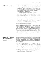
When the advanced treatment is used to compute the upper and
lower confidence intervals for the line of best fit, curves as shown
in
Figure 14.1
1
result. Note that very poor data was purposely used
to get a figure
in
which the
two
confidence intervals are visible.
h
v
x
a,
m
>
S
a,
U
c
a,

Q
a,
U
ii
._
k
+
independent
variable
(x)
I
Figure
14.11
292
A
Guide to Microsoft Excel
2002
for
Scientists and Engineers
the dependent values used
in
the
calibration, and their average
the number
of
x,y
pairs
degrees of freedom
=
n

-
2
The expression for the confidence interval for the computed
Y-
values is:
1
(x-F)2
Note:
Statisticians use the
symbol
h
for the slope and the
Fymbol
a
for
the intercept
in
regression analysis.
This can be confusing
for those
of
The confidence interval for the predicted
x*-
value
is
found using
us
who
use
y

=
mx
+
h
for the
one
of:
CI(Y)
=+t(cG!!)-s,,,
./=
a range named
y
AVERAGE(y)
COUNT( X)
n-2
equation of a straight line.
cqx
*)
=
*t(
a,@).
.
Iml
the slope of the line
the intercept of the line
standard deviation
in
sum of the squares
of the residuals
lSymbol

INDEX(LINEST(y,x,TRUE, TRUE),
1,l)
INDEX(LINEST(y,x,TRUE, TRUE),
1,2)
INDEX(LINEST(y,x,TRUE, TRUE),
3,2)
I
n’
degrees of freedom
the confidence level, generally
0.05
Student’s t-value for given
a
and
df
Ib
INDEX(LINEST(y,x,TRUE, TRUE),
4,2)
a value
TINV(alpha, df)
I
I
s,,
Idf
Ik
1
1
(x*-X)’
-+-+
i

Srx
Cl(X*)
=
+t(a,df).S””.
I4
The variables needed to compute these expressions are shown
in
the table below, together with the appropriate Excel functions.
Purpose
I
Excel
I
the independent values used
in
the
calibration, and their average
a range named
x
AVERAGE(x)
sum of squares of
x
deviations
I
DEVSQ(x)
~
number of repeated
y*
measurements
1
COUNT(range)

I
We begin by using the calibration data from the previous exercise
and computing the confidence levels.
Statistics
for
Experimenters
293
(a)
Copy
Al:B8
from Sheet8 of
CHAPl4.XLS
to
A1
of Sheet9.
Name the
two
ranges
x
and
y.
Enter the text
in
A
1
O:A
19
of
Figure
14.12.

Select
AlO:B19
and name the cells.
Sres
0.095
Figure
14.12
(b)
The required parameters are found with these formulas:
91
1:
912:
913:
914:
91.5:
916:
B17:
B18:
B19:
=INDEX(LINEST(y,
x,
TRUE, TRUE), 1, 1)
=INDEX(LINEST(y,
x,
TRUE, TRUE), 1,2)
=COUNT(x)
=n-2
=INDEX(LINEST(y,
x,
TRUE, TRUE),

3,
2)
=DEVSQ(x)
=AVERAGE(x)
=AVERAGE(y)
0.05
(c) The formulas
in
C4:E4
to compute the predicted
Y-
values and
the upper and lower confidence levels are:
C4:
=A4*m+b
D4:
=$C4
+
TINV(alpha,df)
*
Sres
*
SQRT((
I
/n+($A4-a~gx)~2/Sxx))
E4:
=$C4
-
TINV(alpha,df)
Sres

*
SQRT(( l/n+($A4-a~gx)~2/Sxx))
The mixed cell references
in
D4's
entry
permits copying it to
E4 and then changing the
sign.
The cells C4:E4 are copied
down to
row
8.
294
A
Guide to Microsoft Excel
2002
for
Scientists and Engineers
Finally, we show how to use compute a predicted x-value from a
series of sample measurements.
(d) Enter the text shown
in
CI
1:DIS
of the figure. Enter the
measurements, values in value
C
12:C 16.
These represent five

duplicated analyses of the same sample.
(e) Average they*-values with the
formula=AVERAGE(C12:C16)
in
cell
El
1.
The computed x*-value in
E12
is found with the
formula
=(El
1
-
b)/m
while the confidence intervals
in
E13
and
El
4
are found with:
E13:
=TINV(alpha,df) *
(Sredm)
*
SQRT(l/n
+
1
/COU NT(C 1

2:C
16)
+
(El
1 -avg y)Y/(
mA2*Sxx))
E14:
=TINV(alpha,df)
*
(Sredm)
*
SQRT(l/n
+
I/COUNT(EI
2:
E16)
+
(El 2-a~gx)~2/Sxx)
We have used
two
formulas merely to show they are
equivalent; some texts use one, some the other. The percentage
error (uncertainty)
is computed
in
E15
with =El3/E12 and
formatted as a percentage.
You
will see that this treatment gives aresult that differs somewhat

from that obtained in the previous exercise. We would report the
x*
values as
2.61
f
0.08,
or
2.61,
f
3.,%
at the
95%
confidence
level.
Statistics
for
Experimenters
295
Problems
1.
The distribution ofweight of
1
000
pills from a certain machine
was found to be well described by aNormal curve with a mean
of
400
mg with a standard deviation
of
50

mg.
What fraction
of the pills are expected to be
in
the interval
400
f
10
mg?
2.
An
analysis of substance
X,
thought to be compound
Q,
gave
these results for percentage carbon:
59.09,59.17,59.27,59.13,
59.1,
59.14.
The expected result for compound
Q
is 59.55.
What conclusion can be drawn?
Source of data:
F.
W.
Power,
Analytical Chemistry,
11,

6000
(1
939).
The data has a wide spread by modern standards.
3.
The F-statistic is another measure used to compare data.
As
with the t-statistic, one computes
an
F-value from the data and
compares it to a critical F-value. The null hypothesis (no
difference
in
the means)
is
accepted when the
group
F-value is
less than the critical value. The
Anova:
Single
Factor Data
Analysis tool is one way to do this. The table below represents
the results from three testing laboratories working with the
same sample. Does the Anova result suggest that the mean
values of these results are statistically different?
7.18
7.68

15

Report
Writ
i
n
g
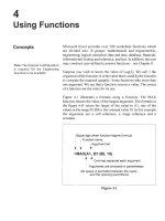
Concepts
Exerc
Paste
:ise
1:
Copy and
The method described
in
this
Exercise will work with Microsoft
Office products such a Word and
PowerPoint. They also work with
many other applications. If
a
simple
Paste does not give the required
result, look
in
the Paste Special
options.
In
this chapter we learn how to place Microsoft Excel workbook
data and charts into a word processor document. There are
two
very different ways to do this:

(i)
using copy and paste, or (ii) with
Object Linking and Embedding
(OLE).
We will examine these
methods
in
detail in the exercises. The algorithm below will help
you choose the appropriate method.
Are you sure that the workbook is complete and the report will
never need updating?
Yes: Use copy and paste.
No:
Will you always have access to the workbook?
Yes: Use linking.
No:
Use embedding.
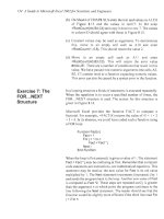
In
this exercise we will copy data and a chart from an Excel
workbook to a document you are writing with a word processor
application such as Microsoft@ Word or Corel@ Wordperfect. We
need a simple workbook with data and a chart. Let
us
assume we
have run an experiment to find the value of a resistor by measuring
the currents passing through the resistor when various voltages are
applied. Since
I
=
V/R,

the slope of a plot of Ivs Vwill be
1/R.
(a) Open a new Excel workbook. Enter the data shown
in
A1
:B11
of
Figure
15.1.
The cell
B11
contains the formula
=I
000/SLOPE(B4: B9,A4:A9)
where the factor of 1000 accounts
for the fact that the current was measured
in
milliamps.
(b) Construct a chart similar to that in Figure
15.1.
Insert a
trendline without the formula being displayed.
Reminder:
In
Microsoft Office
products right-clicking brings up a
(c) Save the workbook as CHAP1
5.XLS.
shortcut menu that is very
convenient for copying and pasting.

(d) Without closing Excel, open your word processor. Put some
text into
a
new document as
in
Figure
15.2
but without the
table
or chart.
298
A
Guide
to
Microsoft
Excel
2002for
Scientists
and Engineers
!AI
B
IC1
0
1
IExperiment
to
find
the
value
of

a
resistor
nl
i
I
I
Figure
15.1
Laboratory Report
1
Finding the value
of
a
resistor using
Ohm’s law
Data.
Voltage
I
Current
(mA)
24.8
32.1
10
40.7
Graph.
I
Current
vs
Vollaae
45

40
35
30
25
20
15
10
5
0
u?
10246810 Vadts
Figure
15.2
(e)
Make Excel the active application. Select the range
A3:B9
in
CHAP1
S.XLS.
Either click the COPY button or use Editlcopy.
(9
Make the word processor active. Move to the line below ‘Data’
and click the Paste button. The data from the Excel worksheet
is inserted into the document
as
a table. You may need to
adjust
its
position and to add any required borders to the table.
Note that the table uses the same font as the worksheet but this

may be changed fiom within the word processor
if
you
so
wish.
Should you need the text not
in
table
form,
use
EditlPaste
-
Special and stipulate non-formatted text. This will give you the
data in tabular columns.
(g) Return to the workbook. Click once on the graph and click the
Copy button.
Report Writing
299
(h) Activate the word processor and move the insertion pointer
under the word ‘Graph’. From the main menu select EditlPaste
-
Special. This will bring up a dialog box similar to that in
Figure
15.3.
Make sure the
Paste
radio button is selected and
in the
As
box select

Picture (EnhuncedMetuJle).
Click the
OK
button. The graph
is
now added to the document as a picture.
It may be positioned and sized to suit your needs using the
word processor commands.
New
to
Excel
2002
Figure
15.3
The Paste Option in Word
2002
may cause a smart tag to be
displayed. This may be used, for example, to change an item
copied as a picture to convert to a linked object.
If you need to copy the same Excel object many times, the
Windows Clipboard can be inconvenient. Recall that an Excel
object remains on the Windows Clipboard only while the
object is selected
-
in the case of a range, only while the ‘ant
track’ is present. The Office Clipboard may be used to hold up
to
24
objects and they are all available in the various Office
components. The command EditlOffice Clipboard may be used

to display the Office Clipboard as a panel in each application.
Exercise
2:
Object
To get the ‘flavour’ of OLE carry out the following:
(a) In the CHAP15.XLS workbook click once on the chart. Click
Embedding
the Copy button.
(b) Move to your word processor and start a new document. Click
the Paste button to copy the chart.
300
A
Guide
to
Microsoft Excel
2002
for
Scientists
and
Engineers
(c) Double click the chart. If you are new to
OLE
the result
is
unexpected. Although you are running a word processor
application (Word, Wordperfect, etc.), the part of the screen
containing the chart now looks like Excel. That
is
exactly what
it

is.
The whole of your Excel workbook has been
embedded
in the document. While the chart
is
open, the application’s
menus and tools bars have been replace by those from Excel.
Your
embedded workbook should consist
of
a chart sheet and
the sheets that were present in the original workbook.
Remember to go back to the chart sheet before closing the
embedded object since this
is
what you want displayed.
(d) If you save the word processing document, a copy
of the
workbook is saved with
it;
not as a separate
file
but as part
of
the word processing document file. You could give a copy of
the
file
to a colleague and he/she could modi6 the workbook
provided hisher computer had Excel installed.
In

the previous exercise we have
embedded
a workbook
in
a
document. Part
of
the word processing ‘space’ has Excel
properties.
In
the embedded object of Exercise
2
we displayed a
chart. We can open the workbook from within the word processing
application, modi@ the data and hence update the chart.
Is
linking
the same? Yes and no! If you
link
a workbook to a
document, the workbook
is
accessible
from
it provided the
workbook file
is
present in the same folder that it was when the
linking was made. One way to think of linking
is

to imagine that
what you
see
in
the document is
a
picture of the part of the
workbook to which it is linked.
Consider the following scenario.
1.
An Excel workbook
is
linked to a Word document on Monday.
Clearly, the workbook and the document display the same data.
2.
On Tuesday, the data
in
the workbook
is
revised. Since the
document
file
is
not open, its data
is
now out of date.
3.
On Wednesday, when the document
is
opened, the word

processor will display a message stating that the document
contains links and asking
if
you wish
to
update them
now.
If
you reply Yes, the workbook
is
opened but you do not see this
happen. The data
is
updated and the workbook
is
closed.
Report Writing
301
Exercise
3:
Embedding and
Linking
Exercise
4:
Creating
an Equation
j-dx
"1
0
X2

Applet:
An applet
is
a small
application
which
must berun
from
within another application.
If nothing was done to the workbook on Tuesday, the same
message would be displayed on Wednesday since the system has
no way
of
knowing if it has been revised since the last time the
document was used.
Linking has certain advantages over embedding:
(1)
it is often
easier to revise the workbook by opening it on its own,
(2)
no
matter what part of the workbook is active, the document displays
the same data it did when the link was first established, and (3) the
document file size is not as large as with embedding.
This is a do-it-yourself exercise. We are near the end
of
the book
and by now you do not need to be told every step. The task
is
to

embed and to link the chart in CHAP15.XLS with a word
processor document and to experiment with the results.
But
I
have not told you how to link! Look at Figure 15.3 and note
the
two
radio buttons.
Paste
results
in
OLE
embedding, Link
results in OLE
linking.
In the
As
box select either Microsoft Excel
Worksheet or Microsoft Excel Chart.
It is also possible to use OLE within a word processing document
with the InsertlQbject

command. You may wish to experiment
with this.
Microsoft provides an applet called Equation Editor which may be
used
in
programs such as Word or Excel to create an equation.
With a little practice and experimentation you will be able to create
complex equations. In this exercise we create the expression at the

left to get you started.
(a) On Sheet2
of
CHAP1 5.XLS, use the command InsertlQbject

and select
Microsoft Equation
3.0.
Figure 15.4 shows how the
worksheet appears.
(b) To draw the integral sign, click the mouse pointer over the
fifth item on the bottom row
of
the Equation Editor toolbar.
Move the pointer to the second item on the top row
of
the drop
down menu since we need an integral sign with
two
limits.
302
A
Guide to Microsoft Excel
2002
for Scientists
and
Engineers
Figure
15.4
(c) Experiment by tapping the key; hold down the

[Shift]
key and tap
[Tab=].
The
L
shape that moves around is the
insertion point.
When a box has something typed in it, the
L
is
reversed. Now use the mouse to move the insertion point to the
box which will hold the lower limit. In this box type
0.
(d) Using either the mouse or
[TabSl,
move to the box where the
upper limit will go. Open the ninth item on the top row of the
toolbar and click on the
x
symbol.
(e) Use
[TabSl
to move the insertion point into the box at the right
of the integral sign. Move the pointer to the second item on the
bottom row of the toolbar and select the first item on the top
row of the drop down menu
-
two open boxes stacked
vertically with a bar between them. We need this template for
the

1/x2
part of the expression.
(f)
Move the insertion point to the top box and type
1.
Move the
insertion point to the bottom box and type
x.
Experiment using
the mouse to relocate the insertion point.
(g) We need an object to hold the superscript. Move to the third
item on the bottom row of the toolbar and select the first item
from the menu. You should now have a superscript box in
which to type the
2.
Alternatively, type the
2,
select it, and
now open the template for a superscript.
(h) Press
[Tab=]
to move the insertion point to the far right of the
equation. Type
dx.
Report Writing
303
Exercise
5:
Interactive Web
(i)

Click the mouse anywhere outside the equation box to close
the Equation Editor applet.
As
you may have discovered, you cannot use
[Spacebar]
when
forming an equation -the applet looks after the spacing
of
items.
You can however, use
@+[XI
to add addition spacing.
By default the Equation Editor uses italics for variables such as
x
and regular font for digits and anything it thinks is a function such
as Exp or Ln. You can enter normal text, including spaces, in an
equation box by using the Text item in the Style menu.
Some users have reported that they have better success if they
compose the equation in Word and copy the completed object
to
the Excel worksheet.
The techniques (Copy and Paste, or Copy and Paste Special) we
used in Exercise
1
may be used to place data and pictures
of
charts
on web pages. Some simple experimenting will quickly show you
the correct method.
Page

Microsoft Excel 2000 and Internet Explorer
4
introduced a new
concept: web pages with interactive Excel. We will briefly explore
this topic but you will need Microsoft FrontPage or a similar web
page composer to develop more complex pages. The HTML files
made in the exercise will be saved on the local hard drive. You
will, of course, need to move them to your web folder if you wish
Internet users to be able to access them.
Figure
15.5
304
A
Guide to Microsoft Excel
2002
for Scientists and Engineers
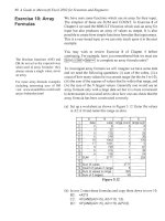
(a) Open Sheet1 of CHAP15.XLS and select the range A1:Dll.
Open the File menu and select
Save
as
Web Page.
This
opens
up a dialog box similar to Figure 15.5. If you merely click the
Save
button, a non-interactive web page will be made.
$
When a web page has previously
been saved
from

an
Excel
(b) Click in the
Selection
radio button$ and
in
the
Add interactivity
be
option box. Enter
Chapl
5.
htm
in
the
Name
box. Click the
Save
button.
called
Republish.
this
button
(c)
Open the Chapl 5.htm file with Internet Explorer (version
4
or
better). The page will be similar to that
in
Figure 15.6.

Experiment by changing some of the values in the table and
noting the change
in
the value
in
B1
1
,
You may wish to ensure that the users can change only certain
cells. Before saving the Excel file as a web page, select the cells
that the user may change and use F~rmatlCglls to unlock them.
Then protect the worksheet using ToolslErotection.
Voltage
Current
(mA)
D
85
16
9
24
8
32
1
8
40
7
I
Sheetl-
_-
Figure

15.6
You may ask why the chart was not included
in
step (a).
Unfortunately, even if it had been included
in
the selection, the
chart would not have appeared on the web page. Putting a chart on
the web page requires a little more work.
Report Writing
305
(d) With the chart selected, open the File menu and click
Save as
Web Page.
Select the
Selection
(or
Republish)
radio button and
put a check mark
in
the
Add
interactivity
box. Use the name
Chapl 5b.htm and click the
Save
button.
(e) When you open the new file with Internet Explorer the chart
and part of the worksheet are visible. However, it is

disappointing to find that only the cell A3:B9 (Le. the ones
used to make the chart) have data
in
them. The chart
is
interactive but we get no value in B
I
1.
The process
in
step (d) gave
us
a web page with a chart but only
those rows of the worksheet needed by the chart are displayed.
So
we will cheat! We will make the chart depend on more cells. We
need the chart to be dependent
on
data
in
row
1
and row
12.
(f)
Move to the worksheet and right click the chart. Select
Source
Data
and open the
Series

tab. Add a new series with x-values
as
El
and y-values as
F1.
Add another new series with
A
12
as
the x-values and B
12
as the y-values. Since there
is
no data in
these cells, the chart
is
unchanged. But as far as Excel
is
concerned the chart
is
dependent on them.
(g)
Repeat step (d) and save the web page as Chapl 5c.htm. Open
the new file with Internet Explorer. Now we have both a chart
and a worksheet that includes all the cells of interest.
To
use Microsoft Excel interactive data on the Web, your users
must have Microsoft Office XP or access to an Ofice XP licence
and the Office Web Components installed. Furthermore, there are
some limitations you should learn about before developing a large

web page. In Excel Help search with the word
Guidelines
and open
the topic
Guidelines and limitations for saving
or
publishing Web
pages.
Strangely, this topic does not show when the phrase
web
page
is
used for the search!
You
may also wish to experiment with using the
Publish
button in
place of
Save.
This offers some options for the web page. It will
generate both an HTML file and a similarly named folder which
hold files needed for the web page.

Answers to Starred Problems
Chapter
2
Chapter
4
Chapter
5

1.
(a)
=2*A1 -C1
(b)
=BIA2 +AI
(c)
=l/(C1"2
-
DI"2)
or
=(CIA2
-
D1"2)"-1
(d)
=
(AI
+
BI)
/
(C1
-
DI)
2.
(a)
=DIA0.5
or
=DIA(1/2)
(b)
=D2"(1/3)
(c)

=D3"(-1)
or
=1/D3
(the latter
is
better)
1.
=ROUNDUP(Length
*
Height
/
2.25)
3
MINVERSE
is an
array formula.
You
should have selected
F3:16,
typed the formula and then pressed
~+[zmJ+[~].
4. =DEGREES(ASlN(OPP/HYPOT))
5.
=FACT(AlO)
/
FACT(A10
-
BIO)
or
=PERMUT(AlO, BIO)

1.
=IF(AI=O,
1,
SIN(X)/X)
or
=IF(Al<>O, SIN(X)/X, 1)
2.
=IF(x<2, IF(y>=lO, IF(y<=l2, IF(r>=O,"Pass","Fail"), "Fail"),
"Fail"), "Fail")
3.
=IF(AND(x<2, AND(y>=IO, y<=12),
z>=O),
"Pass", "Fail")
4.
There are many possible solutions. The simplest is to use:
D2:
=IF(A2+B2=2,1,0),
E2:
=IF(A2+B2>=1
,I
,O)
F2:
=IF(C2+E2=2,1,0),
G2:
=IF(D2+F2>=1,1,0)
Replacing the
Os
and
1
s

by
FALSE
and
TRUE
values
in
the
A,
B
and
C
columns, we could use either of these formulas:
D2:
=AND(A2, B2),
E2:
=OR(A2,B2)
F2:
=AND(C2, D2),
G2:
=OR(D2,F2)
or, with greater risk
of
making an error, we may
use
just
the
D
column with
D2
having the formula:

=OR(AND(A2,B2),AND(C2,OR(A2,
B2)))
308
A
Guide to
Microsoft
Excel
2002
for Scientists and Engineers
Chapter
6
Chapter
7
5. Name the range A3:F15 as ColourCode and enter these
formulas:
A21
:
=VLOOKUP(A19,ColourCode,2,
FALSE)
B2
1
:
=VLOOKUP(Bl S,CoiourCode,2, FALSE)
C2
1
:
=VLOOKUP(Cl S,ColourCode,2, FALSE)
D21:
=VLOOKUP(DlS,ColourCode,2,
FALSE)

A22:
=VLOOKUP(A19,ColourCode,3,
FALSE)
B22:
=VLOOKUP(BlS,ColourCode,4,
FALSE)
C22:
=VLOOKUP(C19,ColourCode,5,
FALSE)
B23:
=(A22*10+822)*C22
C23:
=VLOOKUP(D19,ColourCode,6,
FALSE)
2.
After opening the
Source Data
dialog, move to the
Series
tab.
Click the
Add
button and proceed to add the new data.
Remember you must specify both the y-values and the
x-
values.
3.
Make the chart in the normal manner.
In
an unused part

of
the
worksheet enter
a
pair
ofx-
and y-values in
two
adjacent cells.
Values such as
3
and 0.9 will do. Add these to the chart as a
new data series. The CopylPaste Special method explored
in
Exercise
10
may be use. Alternatively, right click on the chart
and use the Add button
on
Source Data dialog.
Right click on the new point and open the
Format Dataseries
dialog.
On
the
Axis
tab specie
secondary axis.
Return to the
chart and right click. On the

Axes
tab of the
Chart Options
dialog, put
a
Jin
the
Value
(4
axis
box. Format the
two
secondary axes such that they have the same minimum,
maximum and units as their respective primary axis. When all
is
ready, format the new data series to have no line and no
markers
-
to be invisible.
5.
The results are (a) for length vs length:
b
=
I
.0275,
R2
=
0.988,
and (b) for area vs length:
b

=
I
.8065,
R2
=
0.993
1.
You could
plot
Y
against
X
and insert a trendline for a Power model
rather than a Linear model. Ifyou
try
to
make
a
log-log plot
of
the data in the table, a message pops up stating
Negative or
zero values cannot be plotted correctly on log charts.
To
plot
a log-log chart, first multiply the lengths by
10
to give values
in millimetres and the area values
by

100
to give millimetres
squared.
Answers
to
Starred
Problems
309
Chapter 8
1.
The required functions may be coded as shown below.
Function Kelvin(Fahrn)
End Function
Celsius
=
(Fahrn
-
32)
*
5
/
9
Kelvin
=
Celsius
+
273.1
5
Of
course, the two statements could be combined:

Kelvin
=
(Fahrn-32)*5/9
+
273.15
Function Stirling@)
End Function
Stirling
=
n
*
Log(n)
-
n
Function SumRange(a,
b)
If
a
<=
b
Then
lower
=
a:
Else
lower
=
b:
End If
SumRange

=
0
For n
=
lower
To
upper
Next
n
End Function
upper
=
b
upper
=
a
SumRange
=
SumRange
+
n
Note the use
of
the colons
in
SumRange
to place
two
statements
on

one line. The formula
=LN(FUNC(A3))
may be
used to compare the Stirling approximation with the exact
value. When
A3
is
100,
the approximation gives
360.5
while
the exact value
is
363.7.
One cannot test values
of
n
above
170
since
170!
is
close
to
Excel's maximum value
of
1
E+307.
2.
Option Base

1
Function Quad2(a,
b,
c)
Dim Temp(3, 1)
d=(b*b)-
(4*a*c)
Select Case
d
Case
Is
<
0
Temp(
1,
1)
=
"No real"
Temp(2, 1)
=
"roots": Temp(3, 1)
=
'"'
Temp(1, 1)
=
"One root"
Temp(2, 1)
=
-b
/

(2
*
a): Temp(3,
1)
=
""
Temp(1,
1)
=
"Two roots"
Temp(2,
I)
=
(-b
+
Sqr(d))
/
(2
*
a)
Temp(3, 1)
=
(-b
-
Sqr(d))
/
(2
*a)
Case
0

Case Else
End
Select
Quad2
=
Temp
End Function
31
0
A
Guide to
Microsoft
Excel
2002
for
Scientists
and
Engineers
Chapter
9
1
(a)By the principle of mass balance, if
V
ml of water
is
added to
V,
ml of solution of concentration C,, and the concentration of
the resulting solution
is

C,,,
then COY,
=
cb(V
+
V,).
In
this
problem
V,
is always
I,
so
we may write
Cb
=
CJ(
1
+
V).
The required formulas are:
B1
I:
=IF(BlO>req, BlO/(vol+l), NA())
CI
1:
=IF(BlO>req,
C10+(
wash+ vol*disp/lOOO), NAO)
1

(b)From the equation developed
in
(a),
C,
=
Co/(
V
+
I
)
and
C2
=
C,/(
V
+
1).
By substitution, we may
write the last equation as
C2
=
Co/(V+
Continuing with
this, we get
C,
=
Co/(
V+
I
)”.

Take the logarithm of both sides
to find what value of
n
gives the required final concentration.
The formulas are:
B9:
C9:
=(BS*wash
+
B9*A9/1000*disp)
=CEILING( LN( init/req)/LN(AS+ 1
),
1)
We need an integer value
in
B9 but the INT function is not
appropriate; if the formula evaluates
to
4.23 we need
a
value
of
5
not
4
to
ensure that the concentration is equal to or less
than the required value. The
CEILING
or

ROUNDUP
function
is needed.
2.
The equation for the decay
of
iodine-135 integrates to
[I],=[I],
exp(
-k,t).
The series expansion of exp(-x) is
I
-
x
+
x2/2!
-
x3/3!

Hence, provided
-k,t
is
small (Le. small time intervals
and reasonably large half-life), our approximate should give
values of acceptable accuracy. Your graph should resemble
that below.
You
may wish to add these
two
exact solutions to your

worksheet and the chart. The agreement is most satisfactory.
Clearly, when the exact solution to a problem is known, it
should be used rather than an approximation. However, when
a carefully developed approximation agrees with an exact
solution, one has some added confidence that an error did not
slip
into the derivation of the exact solution. The converse is
not necessarily true.