Beginning Microsoft Excel 2010 phần 4 pps
Bạn đang xem bản rút gọn của tài liệu. Xem và tải ngay bản đầy đủ của tài liệu tại đây (904.83 KB, 40 trang )
CHAPTER 4 ■ KEEPING UP APPEARANCES—FORMATTING THE WORKSHEET
106
Figure 4–37. Centered data—centered vertically, that is
click one of the buttons shown in Figure 4–36. What these do is position data along a vertical axis
in the cell—at the bottom of a cell (the default, when you think about it), in the center (as above), or
even at the cell’s ceiling (Figure 4–38):
Figure 4–38. Hitting the heights. Cell data top-aligned
Just bear in mind that if you apply these formats to cells of normal heights, you won’t see the above
effects. That’s because the default row height is too low to enable these to happen, and so you’ll need to
elevate the heights of the rows you want.
How do you do that? The technique is in many ways the right-angled equivalent of the column-
widening methods we described in chapter 2. In order to raise a row height, click on the row’s lower
boundary and drag down (or up, if you want to shrink the row’s height). And if I select several row
boundaries at the same time by dragging along the row numbers, releasing the mouse and then
dragging on any selected row boundary, I’ll see something like this (Figure 4–39):
CHAPTER 4 ■ KEEPING UP APPEARANCES—FORMATTING THE WORKSHEET
107
Figure 4–39. Modulating row heights
I can then modulate the height of all the selected rows at the same—and they’ll all exhibit the
same, new height.
So to achieve the row height you see in Figure 4–40—brought about in cell A10—I simply dragged
down on the lower boundary by the 10 (Figure 4–40):
Figure 4–40. Cell A10, now heightened
And once I’ve engineered the desired height I then clicked the Top Align button—and you get your
top-of-the-cell number. Of course as always I can heighten the row first, click Top Align, and then
enter the number. The sequence of clicks doesn’t matter here.
Now you’ll recall my flippant aside about 48-degree text, the one I threw out on the opening page
of this chapter. Well, if you need or want something like that, look here (Figure 4–41):
Figure 4–41. The Orientation Button
CHAPTER 4 ■ KEEPING UP APPEARANCES—FORMATTING THE WORKSHEET
108
That’s the Orientation button. Click its down arrow, and you’ll see this (Figure 4–42):
Figure 4–42. Orientation options
That’s a pretty illustrative, what-you-see-is-what-you-get drop-down. Select a cell, then click
Vertical Text, for example, and you get (Figure 4–43):
Figure 4–43. Vertical text: Like THIS
And so on. Note, though, that when you call upon these Orientation options they automatically
raise the heights of rows (as also happens with font size changes|) in order to accommodate their
effects, unlike the vertical alignment buttons, which require the user to heighten the rows.
When you click the last Orientation button, Format Cells: Alignment, the aforementioned Format
Cells dialog box appears, with the Alignment tab in view (Figure 4–44):
CHAPTER 4 ■ KEEPING UP APPEARANCES—FORMATTING THE WORKSHEET
109
Figure 4–44. The Alignment tab of the Format Cells dialog box
If you type a number in the Degrees field on the box’s right side and click OK, you can achieve that
48-degree angle, or any other tilt you want, at least between -90 and 90 degrees. You can also click on
the red diamond referenced by the arrow above, and drag it along that Orientation half-circle to angle
your text, too. Either way, you could get the example shown in Figure 4–45:
Figure 4–45. 48 degrees worth of text alignmnent
To turn this effect off—that is, to restore the data to a level orientation—return to the Degrees
field and type “0.”
And if you click that vertical Text field you see beneath the Orientation heading, that’s what you’ll
get—vertical text in their cells, as per the Vertical Text options we saw in the Orientation drop-down
menu in the Alignment Group.
On the left side of the Format Cells dialog are various Text alignment options. Now some of the
options in those Horizontal and Vertical drop-down menus are obscure, but here goes:
General—Brings about standard data alignment defaults, e.g., text is left-aligned, numbers right-
aligned. Obviously you’d only select this to restore realigned data to their original alignments.
Right and Left (Indent)—These simply push, or indent, data in their cells to the right or the left by
the number of characters you type in the Indent field in the dialog box. But just remember that if you
select a right indent, the text will move left, because it is the indent itself that pushes to the right.
CHAPTER 4 ■ KEEPING UP APPEARANCES—FORMATTING THE WORKSHEET
110
Indents can bring about some rather unusual visual results. If I select a right indent and type 10 in the
indent field, I can wind up with something like this (Figure 4–46):
Figure 4–46. Cell-dom used: the indent option
Don’t be fooled—the text is actually “in” the cell selected by the cell pointer. This can’t happen
with a number, however, and for a reason we’ve already discussed in the chapter on data entry; Excel
won’t allow a number to creep into another cell. Thus, if I type 43 in the very cell you see above with
the same indent settings, this is what I’ll get (Figure 4–47):
Figure 4–47. An indented number
Here the indent carries out what’s tantamount to an Auto Fit. The number is indeed indented, but
only within its own cell. Yeah—you’re not likely to use this very often. The two indent buttons (Figure
4–48) found on the Alignment Group on the Home tab of the ribbon:
Figure 4–48. The Indent buttons
equate respectively with the Right and Left Indent options in the Alignment Dialog box—but look at
the buttons. What I’m calling Right Indent features an arrow pointing left, and what I’ve called Left
Indent bears an arrow pointing right. Nevertheless that’s what they are. Moreover, the Alignment
Group caption clinging to the first of the two buttons above (seen when you rest you mouse over it)
calls it Decrease Indent, and not Right Indent; and the other button is labeled Increase Indent; and
CHAPTER 4 ■ KEEPING UP APPEARANCES—FORMATTING THE WORKSHEET
111
neither of these labels corresponds to what the same commands are called in the Alignment Dialog
box.
A couple other qualifications to what is again, not the sort of command you’re likely to call
upon daily: Click the left-pointing indent button arrow in the button group and nothing happens in the
cell at the outset—the data stay put. But click either left or right setting in the dialog box and type a
number in the indent field and the data will indent in the desired direction.
Sorry about that.
Center—Really an equivalent of the Center alignment button. Typing a number in Indent here
has no effect.
Fill—Takes any data you’ve written in the cell and repeats it in the cell, until the cell’s width is
taken up with the data. For example, if I type the word “the” in a cell and select Fill, I’ll see (Figure 4–
49):
Figure 4–49. Filling the cell with data—repeatedly
And if I go on to widen the cell now, I’ll get Figure 4–50:
Figure 4–50. Same command, wider cell.
And yes, you can bring about the same effect with a number—though I can’t imagine why you’d
want to. That is, if I type 3 in a cell and invoke the Fill format I’ll see
333333
across the width of the cell—but its actual value is still….3. Don’t ask questions, but remember—
this is a format, and as such, it doesn’t change the number’s value.
The Justify and Distributed options are similar, though not quite identical to one another. These
commands represent a kind inverse of the column Auto Fit; instead of widening a column to
accommodate its widest entry, Justify and Distributed treat the current column width as a fixed margin
and stack the text in the cell so that it all fits. So for example, if I type (Figure 4–51):
Figure 4–51. Before justifying the text…
And select Justify, the text is realigned like this (Figure 4–52):
CHAPTER 4 ■ KEEPING UP APPEARANCES—FORMATTING THE WORKSHEET
112
Figure 4–52. … and after
The text continues to use the existing column width, and so needs to raise its row height in order to
pinch all the text within that width. The command is called Justify because it emulates a similar effect
in Word, whereby text in a paragraph exhibits straight left and right margins—at least to the extent
possible. Distribution differs only in that it attempts to distribute the text equally across each line in the
cell, so that each line spans the current column width, including the last line—again, to the extent
possible. Here’s another instance of a justified cell (Figure 4–53):
Figure 4–53. Justified vs. Distributed text
And here’s the same test subject to the Distributed option (Figure 4–54):
CHAPTER 4 ■ KEEPING UP APPEARANCES—FORMATTING THE WORKSHEET
113
Figure 4–54. The text, Distributed
Note how the word “happen” is centered here. It’s the closest Distribute could come to spanning
the entire column width with that one word. Try typing the above phrase, applying the Justify and
Distribute effects, and widening the column.
Center Across Selection centers a cell entry across a range of cells. That is, if I type this:
This is how to center data across a selection
in cell E28, and then select this range (Figure 4–55):
Figure 4–55. Data about to be centered across a range selection
And select Center Across Selection, I’ll view this (Figure 4–56):
Figure 4–56. The data, now centered
CHAPTER 4 ■ KEEPING UP APPEARANCES—FORMATTING THE WORKSHEET
114
The effect is clear. Excel treats the selected range as a single space—in essence as one big cell,
even though each cell retains its own identity— and centers the data accordingly. You may want to
contrast this with the Merge & Center command coming up soon.
Of the five Vertical Alignment drop-down options in our dialog box (Figure 4–57),
Figure 4–57. Vertical cell alignment options
the first three—Top, Bottom and Center—are clones of the Vertical Alignment buttons we’ve already
seen in the Alignment Group. The other two—Justify and Distributed—attempt to realize the same
effects as their similarly-named Horizontal options, but to appreciate how they work you need to
tinker with column widths and text length. Here are two examples (Figures 4–58 and 4–59):
Figure 4–58. Vertically distributed text
CHAPTER 4 ■ KEEPING UP APPEARANCES—FORMATTING THE WORKSHEET
115
Figure 4–59. Text, vertically jusftified
The three Text control options in the Alignment dialog box are variations on themes we’ve
previously sounded. As with Justify and Distribute, Wrap text regards a cell’s current width as a
margin, and wraps cell text accordingly. The difference here is that Wrap text doesn’t try to flatten the
right text margin, but rather lets text advance unevenly against cell’s right boundary (Figure 4–60):
Figure 4–60. Wrapping and styling: text wrapped in its cell
Wrap text allows text to wrap naturally to the next line, and doesn’t try the spacing heroics of
Justify or Distribute; this command is represented by the Wrap Text button in the Alignment Group.
Those options—Wrap text, Justify, and Distribute—that realign text by raising row heights instead
of stretching column widths do serve a real purpose. They’re usefully applied to worksheets in which
you want to present data in a series of columns and maintain the same width for all of them, even as
the data in the columns exhibit various widths.
Shrink to fit is a curious flip side to the workings of Wrap text and column Auto Fit. Whereas Wrap
text tries to pile text into a cell without changing its width by raising its row height instead, and Auto Fit
tries to widen columns to accommodate all text in one cell, Shrink to fit changes neither col umn width
nor row height; it shrinks text in order to gather it all into existing width and height. So if you start with
this (Figure 4–61):
CHAPTER 4 ■ KEEPING UP APPEARANCES—FORMATTING THE WORKSHEET
116
Figure 4–61. Text, normally sized
Shrink to Fit will recast the text to look like this (Figure 4–62):
Figure 4–62. Look honey, I shrunk the text
Well, you get the idea.
Finally, the Merge cells option does as it says. It actually consolidates, or merges, selected
contiguous cells into one mega cell. Thus if I start with this entry in cell J12 (Figure 4–63):
Figure 4–63. Text in cell J12
And I then select cells J12 through N12 and click the Merge cells command, I get (Figure 4–64):
Figure 4–64. A merged cell
And what you’re looking at now is all J12; all the selected cells have been absorbed by one cell—
J12—in which I typed my data. All of which raises a fairly obvious question: what does that do for me?
Answer: not much.
But what you really may want to do is merge these cells as we’ve demonstrated above, and then
center the data in the new, super-sized cell. And indeed, there’s an Alignment Group button—Merge &
Center—which does exactly that (Figure 4–65):
Figure 4–65. The Merge & Center button
CHAPTER 4 ■ KEEPING UP APPEARANCES—FORMATTING THE WORKSHEET
117
By default, clicking Merge & Center on our selection of J12 through N12 brings about (Figure 4–
66):
Figure 4–66. A mega, merged cell
This option resolves an old spreadsheet problem—the need to center a title over a collection of
columns (Figure 4–67):
Figure 4–67. How to center that title over all those months?
In the old days, users had to resort to all manner of contortions in order to situate that title in the
middle of the row above the month names, including trying to locate a “middle” column. But we’re
working with 12 columns here, aren’t we? There is no middle column. Merge & Center will turn A1:L1
into one cell (of course that’s the range you need to select), after which Monthly Sales will be precisely
centered within the new super cell—which is still called A1.
The drop-down menu attaching to Merge & Center affords three additional options. Merge Across
allows you to Merge & Center data in consecutive rows. Thus if you start with this (Figure 4–68):
Figure 4–68. Text, one word per cell
You see that I’ve already selected the cells to be merged. Clicking Merge & Center: Merge Across
results in this (Figure 4–69):
CHAPTER 4 ■ KEEPING UP APPEARANCES—FORMATTING THE WORKSHEET
118
Figure 4–69. Each row, its selected cells merged
The respective rows are merged—but here, you see that the data in them are centered. At this
point, you need to then click the standard Center button in the Alignment Group in order to center
each bit of data in each new merged cell in each row. Inelegant, but it works.
Merge & Center: Merge Cells duplicates the Merge cells command we described above in the
Alignment Dialog Box, and Merge & Center: Unmerge Cells returns all cells back to their original
integrity.
An important additional note about the Merge Cells options: Be sure that only the leftmost of the
cells you wish to merge has data in it. Thus if I want to merge cells J12 through N12, and any cells other
than J12 have data in them, those data will be lost when you go ahead with the merge—though Excel
will war n you about this prospect with an onscreen message.
Excel Has Got Your Number(s)
Now that we’ve gotten ourselves oriented and aligned, we can push on to a group whose modest
bearing belies its importance—the Number group (Figure 4–70):
Figure 4–70. The Number button group
Needless to say, formatting numbers is a pretty essential Excel task, but with a couple of slightly
pause-giving exceptions, the task is pretty easy. And the number formats you’re most likely to need are
a snap.
Let’s start with the group’s lower tier, moving left to right. That first button, picturing a pile of
coins and a bank note of indeterminate origin, enables you to format numbers in currency mode—but
unfortunately it’s called, rather cryptically, Accounting Number Format, with its caption asking you to
“Choose an alternate currency format for the selected cell” (of course you know that means cells, too).
That term “alternate” is pretty cryptic, too—but what it means here simply is that clicking the button
will impart a currency motif from one monetary system—Euro instead of Dollars, for example. (But as
we’ll see, there’s a slightly different format out there called Currency, too—but we’ll get to that.)
If you select a cell or a range of cells and click the Accounting Number Format, this is what
happens by default:
CHAPTER 4 ■ KEEPING UP APPEARANCES—FORMATTING THE WORKSHEET
119
• The number is now embellished by your indigenous currency symbol. If you’re
in the States, you’ll see the dollar sign, in the UK the pound sign, and so on (how
Excel knows what symbol to use is tied to your system setup in Control Panel).
• If the number exceeds 999, commas will punctuate where necessary, e.g.,
1,234,582. (In France, the comma is replaced by a space. It’s another country-
specific, Control Panel thing).
• The number will exhibit two decimal points. Thus 27 will appear as 27.00, 678.1
as 678.10.
And why the term Accounting? Well, to repeat—this is a currency-specific format, but of a special
type. What’s special—or at least different—about it is that it lines up the currency symbol independent
of the length of numbers. Consider this example: If I stack these numbers in a column (Figure 4–71):
Figure 4–71. Numbers, pre-formatted
And I click Accounting Number Format, I’ll see (Figure 4–72):
Figure 4–72. Numbers, as per the Accounting format
Note the position of the dollar signs—all positioned in the far left of their cells, even as the actual
numbers describe various widths (note also how the 12 receives those two decimal points, as does
123.8).
Of course that’s all for starters—and you can stop right there if you’re happy with the defaults. But
if you’re in the US and require a different currency, click the down arrow and some standard,
alternative currency options appear, e.g., the British pound and the Euro.
But if you need something else, click More Accounting Formats (Figure 4–73):
CHAPTER 4 ■ KEEPING UP APPEARANCES—FORMATTING THE WORKSHEET
120
Figure 4–73. The Number tab, in an abridged Format Cells dialog box
We’re back to the Format Cells dialog box, this time showing only one tab. Then click the down
arrow by Symbol and click on any one of the long array of currency formats Excel makes available;
your numbers will take on that denomination, and you’ll note as well that you can add or diminish the
number of decimal points your currency displays, either by typing a number in the Decimal places
field or clicking one of those Spin Box arrows in either direction.
That’s really all there is to the Accounting Number Format, but that’s not all there is to currency
formatting, as we’ll see.
The next button in the Number lineup is Percent Style, and while it’s most easy to use (no drop-
down menu, either!) you need to understand what the style will do to a number. If I type:
41
and select that cell, and click Percent Style, I’ll see:
4100%
And not 41%. That’s because percentages really express a number’s percentage of the number 1—
which is, after all, 100%. Thus our number above—which is 41 times the size of 1—has to turn out to be
4100%. If you were expecting 41%, you will need to have typed .41.
But there is an alternative way to institute the Percent Style. If I type:
41%
in a cell, complete with the percent sign, I will achieve exactly that figure—41 percent.
The next button, Comma Style—symbolized, naturally enough, by the comma—imitates the
Accounting Number Format, minus the currency symbol. Thus if I select a cell containing the number
3457, the comma button will make it look like this:
3,457.00
CHAPTER 4 ■ KEEPING UP APPEARANCES—FORMATTING THE WORKSHEET
121
The following two buttons, Increase Decimal and Decrease Decimal, are simple, too, but a jot more
thought-provoking. With each click, Increase Decimal will indeed add one decimal point to a number—
and that includes numbers that have already received two such points under either of the Accounting
Number Comma Style formats. Thus:
67
will appear as 67.0, 67.00, 67.000, etc., with each successive Increase Decimal click. If you write:
=4/7
your result will initially appear as:
0.571429
in a cell of default column width. If you execute an Auto Fit, you’ll see:
.0571428571
a nine-digit rendition of this repeating decimal (note that the “9”—the last digit in the original six-
digit version above—is replaced by 8571—adding additional precision to the number). But you can add
still more decimal digits—up to 15 meaningful ones in total—to a number, after which 5 additional
zeroes will then appear. But of course unless you’re a currency-exchange high roller or a nuclear
physicist, you’re not likely to need all those extras.
Decrease Decimal works in the opposite direction, paring a decimal point with each click. And that
means, for example, that if you click Decrease Decimal once on this number:
4.56
you’ll see:
4.6
Click Decrease Decimal again and you’ll see:
5
Now what’s the numerical value of that figure? The answer: 4.56, and that’s because—at the risk of
repeating myself—we’re formatting data, and formatting changes the appearance of the data only, not
their value. And that means in turn that if I write the above number in cell A12, and write somewhere
else:
=A12*2
I’ll realize 9.12, not the 10 you might assume on the basis of appearances. And if you want proof of
all this, type 4.56 in A12, click back in A12 and click Decrease Decimal twice, and grab a look at the
Formula Bar. You’ll see 4.56.
And what this could mean is that a printout of a worksheet containing the above activity would
display a 5 in A12 and a calculation showing 9.12, when you multiply A12 by 2—and that could be
rather misleading, to put it mildly. It’s something you need to think about. (It should be added, by the
way, that text entries in cells bearing any of the above number formats will be completely unaffected
by any of this. It’s only when you actually enter a numeric value in such cells that these changes
matter.)
There’s one other clarification to be made about the buttons we’ve examined thus far: that any one
of the buttons overrules the effect of any other. Thus, if I’ve formatted 5457.67 to take on this
appearance:
$5,457.67
CHAPTER 4 ■ KEEPING UP APPEARANCES—FORMATTING THE WORKSHEET
122
and then click Comma Style, I’ll see 5,457.67. If I click Percent Style, I’ll see 545767%, and so on. The
point is that the last format selected takes priority.
Now if you examine the broad strip—called Number Format —sitting atop all these buttons in the
Number group, you’ll view the default entry General (Figure 4–74):
Figure 4–74. The General number format
Click the accompanying drop-down arrow and you’ll see (Figure 4–75)
Figure 4–75. The Number Format drop-down menu
Each of those eleven options (you can’t see that eleventh one—Text—in the screen shot, because
you need to scroll down) introduces formatting variations, some of which you’ve already seen, others
of which need to be explained. And note the More Number Format option at the base of the menu, too;
that also requires a closer look. So let’s move in sequence.
The default General format type is captioned No specific format—and that means General makes
its own guess about what kind of data you’ve entered in a cell. If I type a number, General assumes
that’s exactly what I had in mind—an entry that possesses quantitative value. If I type a prose sentence
in the cell instead, General deems it text in nature. If I type a formula, General treats it as such.
Now at this point you’re probably itching to ask a rather pressing question, because I see a lot of
raised hands out there. You want to know: Isn’t this all completely obvious? Why do we need a format to
make any decision about the data, when the nature of those data is so clear?
The answer is that the data types aren’t always so clear. If I type this:
CHAPTER 4 ■ KEEPING UP APPEARANCES—FORMATTING THE WORKSHEET
123
4/5
that sure looks like text, because it’s missing the tell-tale = sign. But General treats the above
expression as a date, namely:
05-Apr
And similarly, General treats:
4–5
the same way, as that same date. Yes—by rights, the General format could have assigned text status to
these entries, but Excel assumes that users who write such expressions really want to enter dates. And
dates, as we’ll see, are really numbers.
In any case, the General format keeps an open mind about what it is you’ve written, whereas the
other formats are a bit bossier, in the sense that they impose their expectations on the data to the
extent they can.
Thus the Number Format option can’t turn text into a number, but it can turn numerical data
displaying a different format back into a garden-variety number—and it throws in two decimal points
for free. Thus if a cell contains this entry:
34.5%
Clicking that cell and then clicking Number will yield:
.35
See why? Here, Number has really done two things: it’s repealed the percent style, and rounded
off the number to two decimal points—because that what Number does by default. But remember: the
number is really .345. Check out the Formula Bar.
Currency is a cousin of the Accounting Number Format, and we’ve already alluded to it. It differs
from Accounting in one respect: the currency symbol it imparts hugs each number’s first digit, instead
of assigning it to a fixed place in the far left of the cell. Thus our Accounting example of a few pages
back looked like this (Figure 4–76):
Figure 4–76. The Accounting format redux
Click Currency on the same range and you’ll come away with this (Figure 4–77):
CHAPTER 4 ■ KEEPING UP APPEARANCES—FORMATTING THE WORKSHEET
124
Figure 4–77. The Currency format
And you’ll be happy to know we’ve already discussed Accounting.
Dates—The Long and the Short of It
But we’ve yet to discuss the next two formatting alternatives—Short Date and Long Date, which do
require a bit of elaboration. In order to appreciate how Excel formats dates, you need to know that at
bottom, a date is a sequenced number. And the sequence starts with January 1, 1900, a date to which
Excel assigns the numerical value of 1. Any post-January 1, 1900 date you enter in any cell in effect
supplies a count of the number of days that have elapsed between itself and that day 1. Thus May 4,
1972 superimposes a date format over the number 26423.00—the number of days stretching in time
from the baseline January 1, 1900 to May 4, 1972. Put otherwise, May 4, 1972 really is 26423.
As a way of corroborating this point, you’ll note that when you click on a cell containing
numerical data—say 34567—and click the Number Format down arrow, you’ll see something like this
(Figure 4–78):
Figure 4–78. Mark that date
CHAPTER 4 ■ KEEPING UP APPEARANCES—FORMATTING THE WORKSHEET
125
Look closely at the screen shot and you’ll see that each format presents its proposed “version” of
34567, that is, how the number would look were you to select this or that format. And look in particular
at Short and Long Date.
Understanding this formative concept (it probably qualifies as a have-to-know)—that dates are
really numbers—helps you understand in turn that if you write April 6, 2001 in cell A1 (in any date
format) and July 12, 1983 in cell A2, you can then write:
=A1-A2
and realize an answer of 6478, which signifies the number of days between the two dates you’ve
entered—because what you’ve really done here is subtract 30509.00 from 36987.00.
Thus a date format—and again, that’s what it is, a format—masks what’s really a number in date
terms. And so if I write say, 23786 in a cell, select it, and select Short Date, I’ll see:
02/13/1965
That’s the mode of date presentation that Excel calls Short Date. Select that same cell and click on
Long Date, and I’ll see:
February 13, 1965
And if write 7/8 in a cell and select Short Date, I’ll see 07/08/2010. Choose Long Date, and July 08,
2010 emerges. Note in this case 7/8 omits the year; and when one does just that, Excel assumes you’re
referring to a date in the current year. But remember what I said earlier. If I type 7/8 under the General
format—without earmarking any date format at all—I’ll still see a date entry in the cell, because even
the General format thinks you meant to type a date anyway. But this is what you’ll see:
Jul-08
an even briefer format than Short Date. It’s a really short date.
To sum up, Date formats paint a chronological veneer over what is really, when the smoke clears,
just a number. And bear in mind that the inverse applies: if I type 7/8 and Jul-08, I can return to that
cell, click the Number format, and see: 40367.00. But why the two decimal points?
Time Is On Your Side—Yes It Is
I was afraid you’d ask that question, and in order to answer it we need to bump down to the next
formatting selection—Time. To Excel, any time or clock reading in a 24–hour span can be treated as a
fraction of a 24–hour denominator. What does that mean? It means this: if I type.346 in a cell, and then
apply the Time format to that cell, I’ll see:
08:18:14
Yeah, I also found this baffling at first—and second—sight. But think about it: the above clock time
actually represents .346 of a day in hourly terms; that is, 8:18:14 is the time of day which stands for
34.6% of an entire 24–hour span. And to trot out perhaps the simplest illustration, type .5 in that cell,
and format it with Time. You’ll see:
12:00
Get it? That’s noon—exactly half, or .5, of a day.
Thus the Date formats provide a default number with two decimal points, e.g., 32456.00, in order to
enable you to format a cell with either date or time readings. If you enter 31456.17 in a cell and opt for
Short Date, you’ll muster 02/13/1986. But if you select the Time format instead, you’ll see 04:04:48, the
time of day which stands for exactly .17 of an entire day. Choose a Date format, and the original
CHAPTER 4 ■ KEEPING UP APPEARANCES—FORMATTING THE WORKSHEET
126
number—31456.17—extracts and uses only the digits to the left of the decimal point. Choose Time and
only the .17 is used.
And for putting up with all that, you get a break—because we’ve already discussed the next
format—Percentage (even though Excel calls the equivalent button Percentage Style).
The next option, Fraction, is a wee bit tricky. It presents any less-than-whole number in fractional
terms. This:
12.5
would be formatted by Fraction as 12 1/2.
That looks pretty simple, and it is; but by default Fraction rounds off if necessary. That is, the
number:
34.32
will be treated by Fraction as 34 1/3 for starters, and that’s not quite exact. As you’ll see a bit later,
however, there are ways of adjusting this discrepancy.
The penultimate option, Scientific, performs a scientific-notational makeover on a number. Type
567 for example and Scientific gives you:
5.67E+02
Thus 0.67 becomes:
6.70E-01
Notice the plus and minus exponent references.
And finally, Text imputes a text format to whatever you write in the cell. That sounds a bit
gratuitous; after all, how else could you possibly format a prose sentence? True, but Text can also
format numbers as text, although you’re not likely to want to do such a thing—because doing so
compromises the numbers’ mathematical character. However, there are times when numerical data
imported from the Internet assumes textual form, and some tinkering is required in order to restore
their true quantitative status.
Now you’ll also note that the last entry on the Number:General Format drop-down menu is
entitled More Number Formats, and clicking it delivers you to the Number tab in the ubiquitous Format
Cells dialog box (Figure 4–79):
CHAPTER 4 ■ KEEPING UP APPEARANCES—FORMATTING THE WORKSHEET
127
Figure 4–79. The Number tab in the Format Cells dialog box
The Category column simply reiterates the options on the Number Format drop-down menu (with
two exceptions—Special and Custom). Clicking any of these often—but not always—presents the user
with additional formatting variations available under that category. For example, if I click Number, I’ll
see this (Figure 4–80):
Figure 4–80. Accentuating the negative—negative number format options
CHAPTER 4 ■ KEEPING UP APPEARANCES—FORMATTING THE WORKSHEET
128
Note here I can choose the way in which I want negative numbers to appear—in red, accompanied
by a minus sign (the default), or featuring both elements. The Use 1000 Separator option simply allows
you to decide if you want your numbers to utilize a comma when it tops 999. The Date category
augments the Short Date and Long Date possibilities (Figure 4–81):
Figure 4–81. Date formatting options
(Note the discussion about asterisks, too. What it means is that only the asterisked formats are tied
directly to the settings in your computer, meaning in turn that 3/14/2001 in the States would
necessarily appear as 14/03/2001 in the UK. The other, asterisk-free options can be selected on any
computer.)
And Time does the same—broadening the number of ways in which a time can appear in a cell
(Figure 4–82):
CHAPTER 4 ■ KEEPING UP APPEARANCES—FORMATTING THE WORKSHEET
129
Figure 4–82. Time formatting options
A few words about the Fraction category may be in order. I earlier noted that when submitted to
this format, the number 34.32 was rendered as 34 1/3—and that’s not correct. 1/3 is .33, not .32, and
that difference might matter—although again we need to remember that, because we’re “only”
formatting the cell, the value is really 34.32 in any case. But by default Fraction estimates the fractional
equivalent of a decimal up to one digit. If we click on the cell containing 34.32 we’ll see (Figure 4–83):
Figure 4–83. Fraction options
CHAPTER 4 ■ KEEPING UP APPEARANCES—FORMATTING THE WORKSHEET
130
And note the sample captures the actual value in the cell we’ve selected. What’s happening here is
that Fraction starts by treating 34.32 as 34.3—one digit’s worth of a decimal; but if we choose the next
option, Up to two digits, we’ll get (Figure 4–84):
Figure 4–84. Options for representing numbers as fractions
The number is now regarded as the two-digit decimal it truly is, and the sample shows 34 8/25—
or, exactly 34.32.
What about Special? This category automatically formats numbers in one of four motifs (at least for
users in the US): Zip Code, Zip Code+4, Phone Number, and Social Security Number. Special imposes
what is called in Access an input mask on a value, supplying punctuation in the cell that spares the user
the need to do so. Some examples: normally typing a zip code in say, New England, where the codes
begin with zero, poses a problem in Excel, because typing:
04567
is rendered by Excel initially as 4567, with the leading zero eliminated. But select Zip Code from the
Special option, and you get all five digits. Indeed, if you type:
4567
Zip Code will automatically supply the zero. Zip Code +4 lets the user type a nine-digit number,
whereupon Excel will insert the dash between the fifth and sixth digit. As a result, typing:
123456789
yields:
12345-6789
The Phone and Social Security Number options likewise supply dashes at the appropriate points in
a number, so that the user doesn’t have to remember exactly where they go.