Engineering and Scientific Computations Using MATLAB phần 3 ppt

Chapter
2:
MATLAB
Functions, Operators, and Commands
35
Chapter
2:
MATLAB
Functions,
Operators, and Commands
36
By
clicking
MATLAB\general,
we have the Help Window illustrated in Figure
2.3,
and
a
complete description
of
the general-purpose commands can be easily accessed.
Figure
2.3.
Help Window
Chapter
2:
MATLAB
Functions, Operators, and Commands
In
particular,
we

have
37
Chapter
2:
IMA
TUB
Functions,
Operators, and Commands
3
8
In addition to the general-purpose commands, specialized commands
and
functions are used. As
illustrated in Figure
2.4,
the
MAT LA^
environment integrates the toolboxes. In particular, Communication
Toolbox, Control System Toolbox, Data Acquisition Toolbox, Database Toolbox, Datafeed Toolbox, Filter
Design Toolbox, Financial Toolbox, Financial Derivatives Toolbox, Fuzzy Logic Toolbox, GARCH
Toolbox, Image Processing Toolbox, Instrument Control Toolbox, Mapping Toolbox, Model Predictive
Control Toolbox, Mu-Analysis and Synthesis Toolbox, Neural Network Toolbox, Optimization Toolbox,
Partial Differential Equations Toolbox, Robust Control Toolbox, Signal Processing Toolbox, Spline Toolbox,
Statistics Toolbox, Symbolic Math Toolbox, System Identification Toolbox, Wavelet Toolbox, etc.
Chapter
2:
MATLAB
Functions, Operators, and Commands
39
Figure

2.4.
MATLAB
demo
window with toolboxes available
Having accessed the general-purpose commands, the user should consult the
MATLAB
user
manuals or specialized
books
for specific toolboxes. Throughout this book, we will apply and emphasize
other commonly used commands needed in engineering and scientific computations.
As
was shown, the
search can be effectively performed using the
helpwin
command. One can obtain the information
needed using the following help topics:
a
help datafun
(data analysis);
a
help
demo
(demonstration);
a
a
help general
(general purpose command);
a
a

help f unf un
(differential equations solvers);
help graph2d
and
help graph3d
two-
and three-dimensional graphics);
help
elmat
and
help matfun
(matrices and linear algebra);
0
help elfun
and
help specfun
(mathematical functions);
0
help lang
(programming language);
a
a
help polyfun
(polynomials).
help ops
(operators and special characters);
In this book, we will concentrate on numerical solutions of equations. The list of
MATLAB
specialized
functions and commands involved

is
given below.
Chapter
2:
MATLAB
Functions,
Operators, and Commands
40
Function functions and ODE solvers.
Optimization and root finding.
fminbnd
-
Scalar bounded nonlinear function minimization.
fminsearch
-
Multidimensional unconstrained nonlinear minimization,
by Nelder-Mead direct search method.
f zero
-
Scalar nonlinear zero finding.
Optimization Option handling
optimset
-
Create or alter optimization OPTIONS structure.
optimget
-
Get optimization parameters from OPTIONS structure.
Numerical integration (quadrature).
quad
-

Numerically evaluate integral, low order method.
quad1
-
Numerically evaluate integral, higher order method.
dblquad
-
Numerically evaluate double integral.
triplequad
-
Numerically evaluate triple integral.
Plotting.
ezplot
-
ezplot3
-
ezpolar
-
ezcontour
-
ezcontourf
-
ezmesh
-
ezmeshc
-
ezsurf
-
ezsurfc
-
fplot

-
Easy to use function plotter.
Easy to use 3-D parametric curve plotter.
Easy to use polar coordinate plotter.
Easy to use contour plotter.
Easy to use filled contour plotter.
Easy to use 3-D mesh plotter.
Easy to use combination mesh/contour plotter.
Easy to use 3-D colored surface plotter.
Easy to use combination surf/contour plotter.
Plot function.
Inline function object.
inline
-
Construct INLINE function object.
argnames
-
Argument names.
formula
-
Function formula.
char
-
Convert INLINE object to character array
Differential equation solvers.
Initial value problem solvers for ODEs. (If unsure about stiffness, try ODE45
first, then ODE15S.)
ode
4
5

-
Solve non-stiff differential equations, medium order method.
ode23
-
Solve non-stiff differential equations, low order method.
ode113
-
Solve non-stiff differential equations, variable order method.
ode23t
-
Solve moderately stiff ODES and DAEs Index
1,
trapezoidal rule.
odel5s
-
Solve stiff ODES and DAEs Index
1,
variable order method.
ode23s
-
Solve stiff differential equations, low order method.
ode23tb
-
Solve stiff differential equations,
low
order method.
Initial value problem solvers for delay differential equations (DDEs).
dde23
-
Solve delay differential equations (DDEs) with constant delays.

Boundary value problem solver for ODEs.
bvp4c
-
Solve two-point boundary value problems for ODEs by collocation.
1D Partial differential equation solver.
PdePe
-
Solve initial-boundary value problems for parabolic-elliptic PDEs.
Option handling.
odeset
-
Create/alter ODE OPTIONS structure.
odeget
-
Get ODE OPTIONS parameters.
ddeset
-
Create/alter DDE OPTIONS structure.
ddeget
-
Get DDE OPTIONS parameters.
bvpset
-
Create/alter
BVP
OPTIONS structure.
Chapter
2:
MATLAB
Functions,

Operators, and Commands
41
bvpget
-
Get
BVP
OPTIONS parameters.
Input and Output functions.
deval
-
Evaluates the solution of a differential equation problem.
odeplot
-
Time series ODE output function.
odephas2
-
2-D phase plane ODE output function.
odephas3
-
3-D phase plane ODE output function.
odeprint
bvpinit
-
Forms the initial guess for
BVP4C.
pdeval
-
Evaluates by interpolation the solution computed by PDEPE.
odefile
-

MATLAB
v5
ODE file syntax (obsolete).
-
Command window printing ODE output function.
Distinct functions that can be straightforwardly used in optimization, plotti.ng, numerical
integration,
as
well
as
in ordinary and partial differential equations solvers, are reported
in
[I
-
41.
The
application
of
many
of
these functions and solvers will be thoroughly illustrated in this book.
REFERENCES
1.
2.
3.
4.
MTUB
6.5
Release
13,

CD-ROM, Mathworks,
Inc.,
2002.
Dabney,
J.
B.
and Harman,
T.
L.,
Mastering
SIMULINK
2,
Prentice Hall, Upper Saddle River, NJ,
1998.
Hanselman, D. and Littlefield,
B.,
Mastering
MATLAB
5,
Prentice Hall, Upper Saddle River, NJ,
1998.
User’s Guide. The Student Edition
of
I’VI~TLAB:
The Ultimate Computing Environment for Technical
Education,
Mathworks, Inc., Prentice Hall, Upper Saddle River, NJ, 1995.
Chapter
3:
MATLAB

and Problem
Solving
42
Chapter
3
MATLAB
and Problem Solving
3.1.
Starting
MATLAB
As we saw in Chapter
1,
we start MATLAB by double-clicking the
MATLAB
icon:
MATLAB
6.5.lnk
The MATLAB Command and Workspace windows appear as shown in Figure 3.1.
Figure 3.1. MATLAB Command and Workspace windows
The line
Thus,
aa=2,
and Figure 3.2 illustrates the answer displayed.
Chapter
3:
MATLAB
and
Problem
Solving
43

Figure
3.2.
Solution of
aa=a+l
if
a=l:
Command and Workspace windows
For the vector
a=
[
1
2
3
1,
to find
aa=a+l,
we have
Variables, arrays, and matrices occupy the memory.
For
the example considered, we have the
MATLAB
statement
a=
[
1
2
31
;
aa=a+l
(typed in the Command Window). Executing this statement,

the data displayed in the Workspace Window
is
documented in Figure
3.3.
Figure
3.3.
Solution
of
aa=a+l
if
a=
[
1
2
31
:
Command and Workspace windows
For
a three-by-three matrix
a
(assigning all entries to be equal to
1
using the
ones
function, e.g.,
a=ones
(3)
),
adding
1

to all entries, the following statement must be typed in the Command Window to
obtain the resulting matrix
aa:
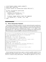
Specifically, as shown in Figure
3.4,
we have
aa
=
I:
:
:1
Chapter
3:
MATLAB
and
Problem
Solving
44
Figure
3.4.
Solution of
aa=a+l
if
a=ones
(3)
:
Command and Workspace windows
Here, the
once
function was used. It is obvious that this function was called by reference from

the
MATLAB
functions library. Call commands, functions, operators, and variables by reference should be
used whenever necessary.
The element-wise operations allow
us
to perform operations on each element
of
a vector. For
example, let
us
add, multiply, and divide two vectors by adding, multiplying, and dividing the
corresponding elements. We have:
Chapter
3:
MATLAB
and
Problem
Solving
45
MATLAB
has operators for taking the real part, imaginary part, or complex conjugate
of
a
complex number. These operators are
real, imag
and
con
j.
They are defined to work element-wise on

any matrix or vector. For example,
using the
sin
and
plot
functions. The corresponding Command and Workspace windows are
documented in Figure 3.5.
Figure 3.5. Solution of
x
=
sin(2r) if
t
=
[0
107~1:
Command and Workspace windows
It is obvious that the size
of
vectors
x
and
t
is
315 (see the Workspace Window in Figure 3.5).
The plot of
x(t)
=
sin(2t) if
r-[0
1

On]
sec is illustrated in Figure 3.6.
Chapter
3:
MTLAB
and
Problem
Solving
46
Figure
3.6.
Plot
ofx
=
sin(2t) if
t=[O
IOx]
sec
MATLAB
does not require any type declarations or dimension statements for variables (as was
shown in the previous example). When
MATLAB
encounters a new variable name, it automatically creates
the variable and allocates the appropriate memory. For example,
The Command and Workspace windows are illustrated in Figure
3.7.
Figilre
3.7.
Command and Workspace windows
Variable names can have letters, digits, or underscores (only the first

31
characters of a variable
name are used). One must distinguish uppercase and lowercase letters because
A
and
a
are not the same
variable.
Conventional decimal notation is used (e.g.,
-
1,
0,
1, 1.1 1,
1.1
1
e
1
1,
etc.). All numbers are stored
internally using the long format specified by the
IEEE
floating-point standard. Floating-point numbers
have a finite precision
of
16
significant decimal digits and a finite range of
1
0-308
to
1

O+308.
Chapter
3:
MTLAB
and
Problem
solving
47
As
was illustrated, MATLAB provides a large number of standard elementary mathematical
functions (e.g.,
abs,
sqrt,
exp,
log,
sin,
cos,
etc.). Many advanced and specialized mathematical
functions (e.g., Bessel and gamma functions) are available. Most of these functions accept complex
arguments. For a list
of
the elementary mathematical functions, use
help elfun
(the MATLAB
functions are listed in the Appendix):
Chapter
3:
h.ta
TLAB
and

Problem
Solving
48
Chapter
3:
MATLAB
and
Problem
Solving
49
3.3.
How
to Use Some Basic
MATLAB
Features
MATLAB
works by executing the statements you enter (type) in the Command Window, and the
To
illustrate the basic arithmetic operations (addition, subtraction, multiplication, division, and
.
In the
MATLAB
Command Window we
type
the following
MATLAB
syntax must be followed. By default, any output is immediately printed to the window.
1+2-e-~+sin5
cos
6

-
7-*
exponentiation), we calculate
statement:
Chapter
3:
MA
TLAB
and Problem Solving
50
3.3.1.
Scalars and Basic Operations with Scalars
Mastering MATLAB mainly involves learning and practicing how to handle scalars,
vectors, matrices, and equations using numerous functions, commands, and computationally
efficient algorithms. In
MATLAB,
a matrix is a rectangular array
of
numbers. The one-by-one
matrices are scalars, and matrices with only one row or column are vectors.
A
scalar
is
a variable with one row and one column (e.g.,
1,
20, or
300).
Scalars are the
simple variables that we use and manipulate in simple algebraic equations.
To

create a scalar, the
user simply introduces it on the left-hand side
of
a prompt sign. That
is,
The Command and Workspace windows are illustrated in Figure
3.8
(scalars
a,
b,
and
c
were
downloaded in the Command Window, and
the
size
of
a,
b,
and
c
is given in the Workspace Window).
Command Window Workspace Window
Chapter
3:
MATLAB
and Problem Solving
51
Figure
3.8.

Command and Workspace windows
MATLAB
fully supports the standard scalar operations using an obvious notation. The following
statements demonstrate scalar addition, subtraction, multiplication, and division.
-b-c;
z
r
3.3.2.
Arrays, Vectors, and Basic Operations
To introduce the vector, let us first define the array. The array is a group of memory locations
related by the fact that they have the same name and same type. The array can contain
n
elements
(entries). Any one of these number (entry) has the “array number” specified the particular element (entry)
number in the array. The simple array example and the corresponding result are given below:
0
array is
(MATLAB
statement):
Chapter
3:
MATLAB
and Problem
Solving
52
MATLAB
allocates memory for all variables used (see the Workspace Window). This allows the
user to increase the size
of
a vector by assigning a value to

an
element that has not been previously used.
For example,
Mathematical operations involving vectors follow the rules of linear algebra. Addition and
subtraction, operations with scalars, transpose, multiplication, element-wise vector operations, and other
operations can be performed.
Chapter
3:
MATLAB
and
Problem
Solving
3.4.
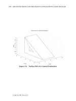
Matrices and Basic Operations with Matrices
Matrices are created in the similar manner as vectors. For example, the statement
53
and the sparsity pattern
of
the matrix
A
is
illustrated in Figure
3.9.
Chapter
3:
MATLAB
and Problem Solving
54
4
0

0.5
1
1.5
2
2.5
3
3.5
nz
=
7
I
Figure
3.9.
Sparsity pattern of the matrix
A
Generating Matrices and Working with Matrices.
Linear and nonlinear algebraic, differential,
and difference equations can be expressed in matrix form. For example, the linear algebraic equations are
given as
qlx1
+
q2x2
+ +
aln-lxfl-l
+a,,x,,
=
bll,
a2p1
+
aZ2x2

+ +
a2n-1~n-l
+
a,x,
=
a,-ll~l
+
an-12~2
+ +
an-ln-I~n-l
+
an+pn
=
bfl-,,
,
anlxl
+
an2x2
+ +
anfl-lxn-l
+
a,xn
=
b,,,
which in matrix form are expressed by
a21
a22
*
a2n-I
a2n

XI
x2
where
x
is the vector of variables,
XER",
x
=
or
Ax=B,
;
A
ER"
"
and
BER"
I
are the matrices of constant
coefficients.
downloaded. The most straightforward way to download the matrix
is
to
create
it
by typing
matrix
=
[valuell valuel2
. .

valueln-l valueln;
where each value can be a real or complex number. The square brackets are used to form vectors and
matrices, and a semicolon
is
used to end a row. For example,
To solve linear and nonlinear equations, the matrices are used. These matrices must be
value21 valuezz
.
.
val~e~~-~ valuepnJ,
Chapter
3:
MATUB
and
Problem
solving
55
Subscript expressions involving colons refer to portions
of
a matrix.
For
example,
A
(
1
:
k,
j
)
represents the first

k
elements
of
the
j
th column
of
A.
The colon refers
to
all row and column elements
of
a matrix, and the keyword
end
refers to the
last row
or
column. Therefore,
sum
(A
(
:
,
end)
)
computes the sum
of
the elements in the last column
of
A.

Chapter
3:
MATLAB
and
Problem
Solving
56
-
-
100
010
001
A=1
11.
111
111
000
-
As
mentioned,
MATLAB
has a variety of built-in functions, operators, and commands to generate
the matrices without having to enumerate all elements. It is easy to illustrate how to use the functions
ones,
zeros,
magic,
etc.
As
an example, we have
Chapter

3:
MATLAB
and Problem Solving
57