Engineering and Scientific Computations Using MATLAB phần 4 ppt

Chapter
3:
MATLAB
and
Problem
Solving
58
because the
AA
is
an active variable.
To
remove
AA
from active variables, we type
Chapter
3:
MATLAB
and
Problem Solving
59
The
size
and
length
functions return the size and length
of
a vector or matrix. For example,
>>
E=magic(4);
SE=size(E),

LE=length(E)
SE
=
LE
=
4 4
4
Chapter
3:
MTLAB
and Problem
Solving
60
Selective
Indexing.
The user may need to perform operations with certain elements
of
vectors
and matrices. For example, let us change all negative elements of the vector or matrix to be positive.
To
perform this, we have
Thus,
y=-4andz=4.5.
The system
of
equations
y+2~=5
3y+4~=6
can be solved graphically. In particular, we have the
following

MATLAB
statement:
>>
y=-10:
z=
(-y+5)
/2
;
plot
(y
ho
z=
1-3
Figure
3.10
illustrates that the solutions
are
y
=
-
4 and
z
=
4.5.
Chapter 4 covers
two-
and three-
dimensional plotting and graphics. The graphical solution is given just to illustrate and verifL the results.
y+2~=5
3y+

42
=
6
Figure
3.10.
Graphical solution of the system of linear equations
Chapter
3:
MATLAB
and Problem
Solving
61
As
another example, using
MATLAB,
let
us
solve the system
of
the third-order
linear
algebraic
equations given
by
Ax=B,whereA=
Our
goal
is to find
x(xl,
x2,

and
x3).
We have
Chapter
3:
MATLAB
and
Problem
Solving
62
Many numerical problems involve the application of inverse matrices. Finding inverse matrices in
MATLAB
is
straightforward using the
inv
function.
For matrix
A=
0
4
0
,
find the inverse matrix, calculate the eigenvalues, derive
[:
1
:i
B
=
10A3A-',
and find the determinant of

B.
Using the inv,
eig,
and
det
functions, we have
ans
=
>>
A=[l
2
3;O
4 0;5 6 71
;
B=lO*(AA
*(-l);
inv(A1, B, eig(B), det(B)
-8.7500e-001 -1.2500e-001 3.7500
0
2.5000e-001
6.2500e-001 -1.2500e-001 -1.2500e-00
1.6000e+002 2.8000e+002
2.4000e+002
0
1.6000e+002
0
4.0000e+002
7.6000e+002 6.4000e+002
8.0816e+000
7.9192e+002

1.6000e+002
1.0240e+006
B=
ans
=
ans
=
Chapter
3:
MATLAB
and
Problem
Solving
63
-0.875 -0.125 0.375
1,
[160 280 2401
0.625 -0.125 -0.125 400 760 640
0.25
B
=
0
160
0
,
the eigenvalues of the matrix
B
are
8.1,
791.9,

160,
and the determinant is
1024000.
We performed the matrix multiplications. The entry-by-entry multiplication, instead of the usual
matrix multiplication, can be performed using a dot before the multiplication operator; for example,
a
.
*
b
.
As
an illustration, let us perform the entry-by-entry multiplication of
two
three-by-three matrices
A=
4
5
6
and
B=
100 1
100
.Wehave
123
10
10 10
[78d
[ill]
The random matrices, arrays, and number generation are accomplished using
rand.

Different
sequences of random matrices, arrays, and numbers are produced for each execution. The complete
description of the
rand
function is available
as
follows:
>>
help rand
RAND Unif
RAND('state',O) resets the generat
RAND('state',J), for integer
J,
re
RAND
(
'state',
sum(
100*clock)
)
resets it
his generator can generate
all
the floa numbers in the
MATLAB
Version
4.x
used random number generators with
a
single seed.

Chapter
3:
WTLAB
and Problem
Solving
64
RAND
(
'seed'
,
0)
and RAND
(
'seed', J) cause the
MATLAB
4
generator to be
used.
RAND('seed') returns the current seed
of
the
MATLAB
4
uniform generator.
RAND('state',J) and RAND('state',S) cause the
MATLAB
5
generator
to
be

used.
See also RANDN, SPRAND, SPRANDN, RANDPERM.
The range of values generated by the
rand
function can be different from what is needed.
R
=
Shifting
+
Scaling*rand
(
)
,
Therefore, scaling is necessary. The general expression for scaling and shifting is
and the following example illustrates the application of the above formula:
>>
R=ones
(5)
+O.
l*rand
('5)
R=
1.0583 1.0226 1.0209 1.0568 1.0415
1.0423 1.0580 1.0380 1.0794 1.0305
1.0516
1.0760
1.0783 1.0059 1.0874
1.0334 1.0530
1.0681 1.0603 1.0015
1.0433 1.0641 1.0461 1.0050 1.0768

The average (mean) value can be found using the
mean
function.
For
vectors,
mean(x)
is the
mean value of the elements in
x.
For
matrices,
mean()()
is a row vector containing the mean value of
each column. In contrast, for arrays,
mean(x)
is
the mean value of the elements along the first non-
singleton dimension of
x.
The median value
is
found by making use of the
median
function.
For
vectors,
median(x)
is
the median value of the elements in x.
For

matrices,
median()()
is a row vector containing the median
value of each column. For arrays,
median(x)
is the median value of the elements along the first
nonsingleton dimension of
x.
>>
R=rand
(5),
Rmean=mean
(R)
,
Rmedian=median
(R)
,
R=
To illustrate the
mean
and
median
functions, the following example is introduced:
0.6756 0.1210 0.2548 0.2319 0.1909
0.6992 0.4508 0.8656 0.2393 0.8439
0.7275 0.7159 0.2324 0.0498 0.1739
0.4784 0.8928 0.8049 0.0784 0.1708
0.5548 0.2731 0.9084 0.6408 0.9943
0.6271 0.4907 0.6132 0.2480 0.4747
0.6756 0.4508 0.8049 0.2319 0.1909

mean
=
Rmedian
=
Thus, using
rand,
we generated the random
5
x
5
matrix
R.
Then, applying the
mean
and
median
functions, we found the mean and median values of each column
of
R.
MATLAB
has functions to round floating point numbers to integers. These functions are
round,
fix, ceil,
and
floor.
The following illustrates the application of these functions:
Chapter
3:
A&
TUB

and
Problem
Solving
65
Symbols
and Punctuation.
The standard notations are used in
MATLAB.
To practice, type the
examples given. The answers and comments are given in Table 3.1.
Table 3.1.
MATLAB
Problems
Problems with
MATLAB
syntaxes
>>
a=2+3
>>
2+3
>>
a=2*3
>>
2*3
>>
a=sqrt (5*5)
>>
sqrt(5*5)
>>
a=1+2j; b=3+4j; c=a*b

>>
a=[O
2 4
6
8
101
>>
a=[0:2:10]
>>
a=0:2:10
>>
a(:)'
>>
a=[0:2:10];
>>
b=a(:)*a(:)'
>>
b(3,4)
>>
b(3,:)
>>
c=b(:,4:5)
Answers
a=5
ans
=
5
a=6
ans
=

6
a=5
ans
=
5
c
=
-5.0000
+lO.OOOOi
a=O
2
4
6
8
10
a=O 2
4
6
8
10
a=O 2 4
6
8
10
a=O
2 4
6
8 10
c=
0

0
0 0 0
0
0
4
8 12
16
20
0
8
16
24
32 40
0
12 24
36
48
60
0
16
32 48
64
80
0
20 40
60
80
100
ans
=

24
ans
=
0
8
16
24 32 40
c=
0
0
12
16
24 32
36 48
48 64
60
80
ans
=
220
Comments
MATLAB
arithmetic
Complex variables
Vectors
Forming matrix
b
Element
(3,4)
Third row

Forming a new matrix
MATLAB
Operators, Characters, Relations, and Logics.
It
was
demonstrated how to
use
summation, subtractions, multiplications, etc. We can use the relational and logical operators.
In
particular, we can apply
1
to symbolize "true" and
0
to symbolize "false." The
MATLAB
operators and
special characters are listed below.
Chapter
3:
MATLAB
and Problem
Solving
66
For
example, the
MATLAB
operators
&,
1,
-

stand
for
"logical
AND",
"logical
OR",
and
"logical
NOT".
Chapter
3:
MTLAB
and
Problem
Solving
67
The operators
==
and
-=
check for equality. Let us illustrate the application of
==
using two
Chapter
3:
MATLAB
and
Problem
Solving
68

Chapter
3:
MATLAB
and
Problem
Solving
69
Polynomial
Analysis.
Polynomial analysis, curve fitting, and interpolation are easily performed.
p(x)
=
1
OX"
+
9x9
+
8x8
+
7x7
+
6x4
+
5x5
+
4x4
+
3x3
+
2x2

+
IX
+
0.5.
We consider a polynomial
To find the roots, we use the
roots
function:
>>
p=[10 9 8 7
6
5
4
3 2 1 0.51;
roots(p)
ans
=
0.6192
+
0.51383.
0.6192
-
0.5138i
-0.7159
+
0.2166i
-0.7159
-
0.2166i
-0.4689

+
0.55973.
-0.4689
-
0.5597i
0.2298
+
0.689Oi
0.2298
-
0.68903.
-0.1142
+
0.6913i
-0.1142
-
0.6913i
As
illustrated, different formats are supported by
MATLAB.
The numerical values are displayed in
15-digit fixed and 15-digit floating-point formats if
format
long
and
format
long
e
are used,
respectively. Five digits are displayed if

format short
and
format short
e
are assigned to be used.
For example, in
format short
e,
we have
>>
format short
e;
p=
[lo
9 8 7 6 5
4
3 2 1 0.51
;
roots(p1
ans
=
6.1922e-001 +5.1377e-0011
6.1922e-001 -5.1377e-001i
-7.1587e-001 +2.1656e-O01i
-7.1587e-001 -2.1656e-001i
-4.6895e-001 +5.5966e-O01i
-4.6895e-001 -5.5966e-001i
2.2983e-001 +6.8904e-O01i
2.2983e-001 -6.8904e-001i
-1.1423e-001 +6.9125e-O01i

-1.1423e-001 -6.9125e-0013.
In general, the polynomial
is
expressed
as
The functions
conv
and
deconv
perform convolution and deconvolution (polynomial
p,(x)=x4 +2x3 +3x2 +4~+5
and
p2(x)=6x2 +7~+8
2
p(x)
=
u,x"
+
u,_,xn-l
+
.
.
.
+
u2x
+
a,x
+
a,.
multiplication and division). Consider two polynomials

To
findp3(x)
=
pl(x)p2(x)
we use the
conv
function. In particular,
>>
pl=[l 2 3 4 51
;
p2=[6 7 81; p3=conv(pl,p2)
p3
=
Thus, we find
6 19 40 61 82 67 40
p,(x)=6~~+19~~+40~~ +61x3+82x2 +67~+40.
=
6x2 +7x+8
=
p,(x)
p
(x)
It is easy to see that
p4(x)
=
3
=
6x6
+
1

9x5
+
40x4
+
61x3
+
82x2
+
67x
+
40
PI
x4 +2x3+3x2 +4x+5
This
can be verified using the
deconv
function. In particular, we have
>>
p4=deconv (p3, pl)
p4
=
6 7 8
Comprehensive analysis can be performed using the
MATLAB
polynomial algebra and numerics.
P,(X)
=6x6 +19x5 +40x4 +61x3 +82x2 +67~+40
For example, let
us
evaluate the polynomial

Chapter
3:
MATLAB
and
Problem
Solving
70
at the points
0,
3,6,9,
and
12.
This problem has a straightforward solution using the
polyval
function. We
have
>>
x=
[O
:
3
:
121
;
y=polyval (p3,
x)
Y=
Thus, the values of
p3(x)
at x

=
0,3,9,
and
12
are
40,14857,496090,462477
1,
and
2359
12
12.
As
illustrated,
MATLAB
enables different operations with polynomials (e.g., calculations of roots,
convolution, etc.). In addition, advanced commands and functions are available, such
as
curve fitting,
differentiation, interpolation, etc. We download polynomials as row vectors containing coefficients
ordered by descending powers.
For
example, we download the polynomial
p(x)
=
x3
+
2x
+
3
as

40
14857 496090 4624771 23591212
>>
p=[l
0
2 31
The following functions
are
commonly used:
conv
(multiply polynomials),
deconv
(divide
polynomials),
poly
(polynomial with specified roots),
pol yder
(polynomial derivative),
pol
yf it
(polynomial curve fitting),
pol yval
(polynomial evaluation),
pol yva
1m
(matrix polynomial
evaluation),
residue
(partial-fraction expansion),
roots

(find polynomial roots), etc.
The
roots
function calculates the roots of a polynomial.
>>
p=
[l
0
2
31
;
r=roots(p)
r=
0.5000
+
1.6583i
0.5000
-
1.65833.
-1.0000
>>
p=poly(r)
P=
The
poly
function computes the coefficients of the characteristic polynomial of a matrix.
For
example,
The function
poly

returns to the polynomial coefficients, and
1.0000
-0.0000
2.0000 3.0000
>>
A=[l
2
3;
0
4
5;
0
6 71; c=poly(A)
c=
1.0000
-12.0000
9.0000
2.0000
The roots of this polynomial, computed using the
roots
function, are the characteristic roots
(eigenvalues) of the matrix
A.
In particular,
>>
r=roots
(c)
r=
11.1789
1.0000

-0.1789
The
polyval
function evaluates a polynomial at a specified value.
For
example,
to
evaluate
p(x)=x3+2x+3
ats=lO,wehave
>>
p=
[l
0
2
31
;
plO=polyval(p,lO)
p10
=
the polynomial
p(x)
=
x3
+
2x
+
3,
the
MATLAB

statement is
>>
p=
[l
0
2 31
;
der=polyder(p)
der
=
The
polyder
function can
be
straightforwardly applied to compute the derivative of the product
or
quotient of polynomials.
For
example, for two polynomials
p,(x)
=
x3
+
2x
+
3
andp2(x)
=
x4
+

4x
+
5,
we
have
>>
pl=[l
0
2 31; p2=[1
0
0
4 51; p=conv(pl,p2), der=polyder(pl,p2)
P=
der
=
1023
The
polyder
function computes the derivative of any polynomial.
To
obtain the derivative of
3
0
2
1
0
2 7 5 8 22 15
7
0
10 28 15 16

22
Chapter
3:
MATLAB
and
Problem
Solving
71
The data fitting can be easily performed. The
polyf
it
function finds the coefficients of a
x=[O 12
3
4
5
6 7 8 9]andy=[1 2.5 2
3
3 3
2.5 2.5 211.
polynomial that
fits
a set of data
in
a least-squares sense. Assume we have the data (x and
y)
as
given by
Then, to fit the data by the polynomial of the order three, we have
>>

x=[O
12
3
4
5
6
7 8
91;
y=[l
2.5 2
3
3
3
2.5 2.5 2
11;
p=polyfit(x,y,3)
P=
Thus, one obtains p(x)
=
0.001x3-
0.
104x2
+
0.8478~
+
1.2028.
>>
plot(x,y,
'-i,x,polyval(p,x)
,':I)

of the data and its approximation by the polynomial are illustrated in Figure
3.1
1.
0.0010
-0.1040 0.8478 1.2028
The resulting plots, plotted using the following
MATLAB
statement,
16-
14~
12-
1
0123456769
Figure3.1l.Plotsofthexydata(x=[O
1
2
3
4
5
6
7
8 9]andy=[1
2.5
2
3
3
3
2.5 2.5 211)
and its approximation by p(x)
=

0.001~~-
0.
104x2
+
0.8478~
+
1.2028
Interpolation (estimation of values that lie between known data points) is important in signal and
image processing.
MATLAB
implements a number of interpolation methods that balance the smoothness of
the data fit with the execution speed and memory usage. The one-,
two-
and three-dimensional
interpolations are performed by using the
interpl, interp2,
and
interp3
functions. The
interpolation methods should be specified, and we have
interpl (x, y, xi,method)
.
The nearest neighbor interpolation method
is
designated by
nearest,
while the linear, cubic
spline, and cubic interpolation methods are specified by the
linear, spline
and

cubic
functions.
Choosing an interpolation method, one must analyze the smoothness, memory, and computation time
requirements.
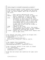
Example
3.4.
I.
Consider the nonlinear magnetic circuit. Ampere's law states that the line integral
of
around the
closed path
is
proportional to the
net current
through the enclosed area. However, the value of permeability
of the ferromagnetic material depends on the external field, and
p
is
not constant. This effect
is
observed due
to the
saturation magnetization
phenomena. In general, one should use the nonlinear magnetization curves.
That
is,
the equation
L
=
-

N@
=
-
v/
=
const
is
valid
only
if the magnetic system
is
linear.
ii
Weuse
i=[O
0.2 0.4 0.6 0.8
1
1.2 1.4 1.6 1.8 21
and
Consider a set of data for the
flux
linkage
-
current relation for an electromagnetic motion device.
0
=[0
0.022 0.044 0.065 0.084
0.1
0.113
0.123 0.131 0.136 0.1381.

Chapter
3:
MATLAB
and Problem
Solving
72
Using
MATLAB,
curve fitting, interpolation, and approximation can be performed (see the script and
the results).
MATLAS
ScriDt
Chapter
3:
MATLAB
and Problem
Solving
73
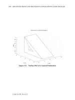
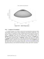
Figure
3.12
plots the data, and the variations
of
the inductance are evident. Approximating
CD
=
f(i)
CD
=
-0.0048i3
-

0.016i2
+
0.12i
-
0.00075
,
by the third-order polynomial
is
found to be
0.1
X
G;
0.05
0
The plot of the Current
-
Flux data
00
0
0
0
0
0
0
0
I
Current
Interpolation of
the
Current

-
Flux curve
by
N-order polynom
Is
X
0
1
2
Current
Derivative dFlux
/
dCurrent as a function of Current
Derivative dFlux
/
dCurrent as a function of Current
I
I
I
1
2
Current
Derivative dFlux
/
dCurrent as a function
of
Current
Figure
3.12.
Application

of
numerical analysis in curve fitting, interpolation,
and
approximation
3.5.
Conditions and
Loops
The logical operators in
MATLAB
are
<,
>,
<=,
>=,
==
(logical equals),
and
-=
(not equal). These
are binary operators which return the values
0
and
1
(for scalar arguments).
To
illustrate them, we have
Chapter
3:
MATLAB
and Problem Solving

74
These logical operators have limited features, and therefore, loops, conditions, control statements, and
control structures (sequence, selection, and repetition structures) are embedded
in
all programming
languages. In particular,
MATLAB
has standard
if-elseif-else, switch,
and
while
structures.
The general form of the pseodocode for the
if
conditional statement
is
Control Structures.
The
if
selection structure (conditional statement) allows us to design
programs that make decisions about what commands to execute. This decision-making is performed
choosing among alternative actions based upon the particular (specific) conditions. The basic statement,
to illustrate the basic features,
is
if
a>O
x=aA3;
end
Chapter
3:

MATLAB
and
Problem
Solving
75
Thus, we assign
x
be the equal
to
a3
if
a
is
positive. We have an
end
statement
to
terminate the
program. We define an
else
clause which
is
executed
if
the condition given
(if
statement) is not true.
For example,
if
a>O

x=a"3;
else
x=-aA4;
end
Hence,
if
a
=
5,
x
=
125,
and
if
a
=
-
5,
x
=
-
625.
Here, we need one
end.
Using the
MATLAB
help, we have:
1.
if
structure:

>>
help if
IF IF statement condition.
The general form
of
the IF statement is
IF expression
statements
ELSEIF expression
statements
ELSE
statements
END
The statements are executed if the real part of the expression
has all non-zero elements. The ELSE and ELSEIF parts are optional.
Zero or more ELSEIF parts can be used as well as nested IF'S.
The expression
is
usually of the form expr rop expr where
rop
is
==,
<,
>,
<=,
>=,
or
-=.
Ex
amp

1
e
if I
==
J
elseif abs(1-J)
==
1
else
end
A(1,J)
=
2;
A(1,J)
=
-1;
A(1,J)
=
0;
See also RELOP, ELSE, ELSEIF, END, FOR, WHILE, SWITCH
2.
e
1
se
structure:
>>
help else
ELSE Used with IF.
ELSE is used with IF. The statements after the ELSE are executed
if all the preceding IF and ELSEIF expressions are false.

The general form
of
the IF statement is
IF expression
statements
ELSEIF expression
statements
ELSE
statements
END
See also IF, ELSEIF, END.
Chapter
3:
MATLAB
and
Problem
Solving
76
3.
>>
help elseif
e
1
s
e
i
f
structure:
ELSEIF IF statement condition.
ELSEIF is used with IF. The statements after the ELSEIF are

executed if the expression is true and all the preceding IF and
ELSEIF expressions are false. An expression is considered true if
the real part has all non-zero elements.
ELSEIF does not need a matching END, while ELSE IF does.
The general form of the IF statement is
IF expression
statements
ELSEIF expression
statements
ELSE
statements
END
See also IF, ELSE, END.
4.
switch
structure:
>>
help switch
SWITCH Switch among several cases based on expression.
The general form of the SWITCH statement is:
SWITCH switch-expr
CASE case-expr,
CASE {case-exprl, case-expr2, case-expr3,

)
statement,
. .
.
,
statement

statement,
,
statement

OTHERWISE,
statement,
,
statement
END
The statements following the first CASE where the switch-expr matches
the case-expr are executed. When the case expression is a cell array
(as in the second case above), the case-expr matches if any of the
elements of the cell array match the switch expression. If none
of
the case expressions match the switch expression then the OTHERWISE
case is executed (if it exists). Only one CASE is executed and
execution resumes with the statement after the END.
The switch-expr can be a scalar or a string.
matches a case-expr if switch-expr==case-expr. A string
switch-expr matches a case-expr if strcmp(switch-expr,case
-
expr)
returns
1
(true).
A scalar switch-expr
Only the statements between the matching CASE and the next CASE,
OTHERWISE, or END are executed. Unlike C, the SWITCH statement
does not fall through
(so

BREAKS are unnecessary).
Example
:
To execute a certain block of code based on what the string, METHOD,
is set to,
Chapter
3:
MATLAB
and
Problem
Solving
77
method
=
'Bilinear';
switch lower (METHOD)
case {'linear', 'bilinear')
disp('Method is linear')
case 'cubic'
disp('Method is cubic')
case 'nearest'
disp('Method is nearest')
otherwise
disp('Unknown method.')
end
Method is linear
See also CASE, OTHERWISE, IF, WHILE, FOR, END.
The following conclusions can be made.
1.
2.

3.
The
if
selection structure performs an action if a condition is true
or
skips the action if the
condition is false.
The
if
-
else
selection structure performs an action if a condition is true and performs a
different action if the condition is false.
The
switch
selection structure performs one of many different actions depending on the value
of an expression.
Therefore, the
if
structure
is
called a single-selection structure because it performs (selects)
or
skips
(ignores) a single action. The
if
-
else
structure is called a double-selection structure because it
performs (selects) between

two
different actions. The
switch
structure is called a multiple-selection
structure because it selects among many different actions.
Using the results given it
is
obvious that we can expand the
if
conditional statement (single-
selection structure) using other possible conditional structures. If the first condition
is
not satisfied, it
looks for the next condition, and
so
on, until it either finds an
e
1
se,
or
finds the
end.
For
example,
if
a>O
x=a"3;
elseif
a==O,
else

x=j;
x=-aA4;
end
This script verifies whether
a
is positive (and, if
a>O,
x=a3),
and if
a
is not positive, it checks whether
a
is
zero (if this is true,
x
=
j
=
fi
).
Then, if
a
is
not zero, it does the else clause, and if
a<O,
x=
-
a4.
In
particular,

a=2;
if
a>O
x=a"
3
:
el sei
f
a==O
,
else
end:
x
gives
x=j:
x=-a"4
:
x=
8
Chapter
3:
MATLAB
and
Problem
Solving
78
while
a=O;
if
a>O

x=a"3;
elseif
a==O,
else
end; x
results
in
x=j;
x=-a"4;
x=
0
t
1.OOOOi
In addition
to
the selection structures (conditional statements), the repetition structures
while
and
for
are used
to
optimize and control the program. The
while
structure is described below:
>>
help while
WHILE Repeat statements an indefinite number of times.
The general form of a WHILE statement is:
WHILE expression
END

statements
The statements are executed while the real part of the expression
has all non-zero elements. The expression is usually the result
of
expr rop expr where rop is
==,
<,
>,
<=,
>=,
or
-=.
The BREAK statement can be used to terminate the
loop
prematurely.
For example (assuming
A
already defined):
E
=
O*A;
F
=
E
+
eye(size(E)); N
=
1;
while norm(E+F-El
1)

>
0,
E=E+F;
F
=
A*F/N;
N=N+1;
end
See also
FOR,
IF, SWITCH, BREAK, END.
Thus, the
while
structure repeats
as
long
as
the given expression
is
true (nonzero):
Chapter
3:
MATLAB
and Problem Solving
79
The built-in function
disp
displays the argument. The loop is terminated by the
end.
The

for
structure allows you to make a loop or series
of
loops
to be executed several times. It is
functionally very similar to the
for
structure in
C.
We may choose not to use the variable
i
as
an index,
because you may redefine the complex variable
i
=
fi.
Typing
for
z
=
1:4
k
end
causes the program to make the variable
z
count from
1
to
4,

and print its value
for
each step.
For
the
above statement, we have
z=
1
2
3
4
z=
z=
z=
In general, the loop can be constructed
in
the form
for i=l:n, <program>, end
Here we will repeat program
for
each index value
i.
>>
help for
The complete description
of
the
for
repetition structure
is

given below:
FOR Repeat statements a specific number of times.
The general form of a FOR statement is:
FOR variable
=
expr, statement,
.
.
.,
statement END
The columns
of
the expression are stored one at a time in
the variable and then the following statements, up to the
END, are executed. The expression is often of the form X:Y,
in which case its columns are simply scalars. Some examples
(assume N has already been assigned a value).
FOR
I
=
l:N,
FOR
J
=
l:N,
END
A(1,J)
=
l/(I+J-I);
END

FOR
S
=
1.0:
-0.1:
0.0,
END
steps
S
with increments
of
-0.1
FOR E
=
EYE(N),

END sets
E
to
the unit N-vectors.
Long loops are more memory efficient when the colon expression appears
in the FOR statement since the index vector is never created.
The BREAK statement can be used to terminate the loop prematurely.
See
also
IF, WHILE,
SWITCH,
BREAK, END.
several times. You can have nested
for

structures.
For
example,
for
m=1:3
The loop must have a matching
end
statement
to
indicate which commands should be executed
for
n=1:3
x
(m,
n) =mtn*i;
end
end;
x
Chapter
3:
MATLAB
and
Problem
Solving
80
generates (creates) the x matrix
as
x=
9
17

25
10
18
26
11
19
27
To
terminate
for
and
while,
the
break
statement is used.
3.6.
Illustrative
Examples
Example
3.6.1.
Find the values
of
a,
b,
and
c
as
given by the following expressions
-1
a

=
5x2
-
6y
+
72,
b
=
3Y2
mdc=(l+-$)
4x
-
52
ifx=
10,y=-20
andz=30.
Solution.
In the
MATLAB
Command Window, to find a, we type the statements
0
Example
3.6.3.
Given the complex number
N
=
13
-
7i.
Using

MATLAB,
perform the following numerical
Find the magnitude
of
N.
Find the phase angle of
N.
Determine the complex conjugate
of
N.
calculations:
a.
b.
c.