how to do everything with ms office excel 2003 phần 3 pdf

Enter Data with Paste, Paste Options, and Paste Special
You can cut, copy, and paste data from the Windows Clipboard or the Clipboard task pane much
as in the other Office applications but with the following variations:
■
When you copy an item, Excel displays a flashing border around it to indicate that the
item is available for pasting. To paste a single time without using the Clipboard task
pane, select the destination and press
ENTER; Excel removes the flashing border and
clears the item from the Clipboard. To paste multiple times, issue a Paste command (for
example,
CTRL-V). Excel maintains the flashing border until you clear it by pressing ESC.
■
When you paste the contents of multiple cells, Excel uses the active cell as the top-left
corner of the destination range. So you don’t need to select the whole of the destination
range, just its top-left cell.
■
When you paste data, Excel displays a Paste Smart Tag below and to the right of the
destination cells. Click this Smart Tag to display a menu of paste options, as shown
below. For example, you can choose between maintaining the formatting of the source
cell and matching the formatting of the destination cell, apply formatting only, or paste a
value rather than the formula that produces it. The available options depend on the type
of data you’ve pasted.
When the Smart Tag options don’t give you the fine control you need, issue a Paste Special
command from the Edit menu or the shortcut menu to display the Paste Special dialog box:
70 How to Do Everything with Microsoft Office Excel 2003
HowTo-Tght (8) / How to Do Everything with Microsoft Office Excel 2003 / Hart-Davis / 3071-1 / Chapter 3
P:\010Comp\HowTo8\071-1\ch03.vp
Thursday, August 28, 2003 11:35:52 AM
Color profile: Generic CMYK printer profile
Composite Default screen
3

CHAPTER 3: Create Spreadsheets and Enter Data 71
HowTo-Tght (8) / How to Do Everything with Microsoft Office Excel 2003 / Hart-Davis / 3071-1 / Chapter 3
The Paste section of the Paste Special dialog box offers these mutually exclusive options:
■
All Pastes everything copied: all values, formulas, formatting, etc.
■
Formulas Pastes all data—formulas, constants, etc.—without formatting.
■ Values Pastes the values of formulas (rather than the formulas themselves)
without formatting.
■
Formats Pastes all formatting without any data or formulas.
■
Comments Pastes all comments without other data.
■
Validation Pastes the data-validation criteria.
■
All Except Borders Pastes all data and formatting except cell borders.
■
Column Widths Pastes the column widths without data and without other formatting.
■
Formulas and Number Formats Pastes formulas and number formatting only.
■
Values and Number Formats Pastes values and number formatting only.
The Paste Special dialog box limits you to a single operation at a time, but you can use
multiple Paste Special operations with the same data range to transfer multiple items.
The Operation section of the Paste Special dialog box offers mutually exclusive options for
adding, subtracting, multiplying, dividing, or performing no operation (the default). To use these
options, follow these steps:
1. Copy to the Clipboard the cell or range that contains the number or numbers you want to
add to or subtract from, or by which you want to multiply or divide, the other numbers.

P:\010Comp\HowTo8\071-1\ch03.vp
Thursday, August 28, 2003 11:35:53 AM
Color profile: Generic CMYK printer profile
Composite Default screen
2. Select the cell or range you want to affect.
3. Display the Paste Special dialog box, choose the appropriate Operation option, and click
the OK button.
The final section of the Paste Special dialog box contains the following options, which you
can use with the Paste options and Operation options:
■
Skip Blanks Prevents Excel from pasting blank cells.
■
Transpose Transposes rows to columns and columns to rows.
Link Data Across Worksheets or Across Workbooks
Chances are, your work in Excel involves a healthy variety of different worksheets or workbooks,
some of which bear a relationship to one another. To avoid having to copy information manually
from one worksheet or workbook to another each time it changes (let alone retype it), Excel lets
you link data across worksheets or even across workbooks. For example, each departmental
manager might maintain a separate workbook of productivity targets, with summaries from each
of those workbooks linked to an executive-overview workbook used by the VPs.
To create a link, follow these steps:
1. Open the source workbook and the destination workbook. (If you’re linking from one
sheet of a workbook to another, open just that workbook.)
2. In the source workbook, copy the relevant cell or range.
3. Display the destination sheet of the destination workbook, issue a Paste Special
command to display the Paste Special dialog box, and click the Paste Link button.
Excel updates links within the same workbook automatically and immediately when you change
the data in the source. When you link from one workbook to another, here’s what happens:
■
If the source workbook is open and contains changes made since the destination

workbook was last updated, Excel updates the links in the destination workbook
when you open it.
■
If the source workbook isn’t open but contains changes made since the destination
workbook was last updated, Excel’s default behavior is to prompt you to update
automatic links when you open the destination workbook. To make Excel update the
links without prompting, clear the Ask to Update Automatic Links check box on the
Edit tab of the Options dialog box.
You can also force updating manually by choosing Edit | Links and working in the Edit Links
dialog box. This dialog box also lets you check the status of a link, change a link’s source, or
break a link (for example, if the source isn’t available now and never will be again). See “Edit,
Update, and Break Links,” in Chapter 16, for more information on working with links.
72 How to Do Everything with Microsoft Office Excel 2003
HowTo-Tght (8) / How to Do Everything with Microsoft Office Excel 2003 / Hart-Davis / 3071-1 / Chapter 3
P:\010Comp\HowTo8\071-1\ch03.vp
Thursday, August 28, 2003 11:35:53 AM
Color profile: Generic CMYK printer profile
Composite Default screen
3
Use AutoFill to Enter Data Series Quickly
To enable you to fill in series of data quickly and easily in worksheets, Excel provides the
AutoFill feature. You select one, two, or more cells that contain the basis for a series, then drag
the AutoFill handle—the black square that appears at the lower-right corner of the last cell
selected—to show AutoFill the range of cells you want to fill with the series of data. AutoFill
analyzes the starting cells, determines what the contents of the other cells should be, and enters
the information automatically.
The best way to get the hang of AutoFill is to play around with it for a few minutes. Open a
new, blank workbook and try the following examples to see how AutoFill works and what it does:
■
Enter January in cell A1 and drag the AutoFill handle to cell D1. As you drag, AutoFill

displays a ScreenTip to show you the entry that the current cell will receive. When you
release the mouse button, AutoFill enters the months February through April in the
selected cells.
■
Press CTRL-Z to undo the AutoFill operation, and then drag the AutoFill handle from cell
A1 to cell M1 instead. AutoFill will start repeating the list and enter January in cell M1.
■
Enter 0 in cell A2 and 5 in cell A3, select those cells, and then drag the AutoFill handle
down column A. AutoFill continues the sequence by adding 5 to each number it enters in
the successive cells.
The AutoFill series must be contained in a single row or a single column—it can’t cover
a range consisting of multiple rows and columns at once.
■
Drag the AutoFill handle from cell A3 to the right. AutoFill repeats the data in cell A3
(the number 5), because there’s no progression. You can use this behavior to extend a
text label over a range of cells.
■
Hold down CTRL and drag the AutoFill handle from cell A3 to the right. Holding down
CTRL forces AutoFill to increment the number entered in the single cell over the AutoFill
range rather than copy the number.
■
Enter Monday in cell B2 and press CTRL-B to make it boldface. Then right-drag the
AutoFill handle across to cell H2 and release the mouse button. AutoFill displays a
context menu that includes options such as Copy Series, Fill Series, Fill Formatting
Only, Fill Without Formatting, Fill Days, and Fill Weekdays. (For other content, the
options Fill Months, Fill Years, Linear Trend, Growth Trend, and Series are available as
appropriate.) Select the appropriate item. For example, select Fill Formatting Only to fill
the series with the formatting from cell B2 but skip filling the cells with the content.
You can change the item that AutoFill has entered by clicking the AutoFill Options Smart
Tag that appears below and to the right of the last cell in an AutoFill series and choosing the

appropriate option from the resulting menu.
CHAPTER 3: Create Spreadsheets and Enter Data 73
HowTo-Tght (8) / How to Do Everything with Microsoft Office Excel 2003 / Hart-Davis / 3071-1 / Chapter 3
P:\010Comp\HowTo8\071-1\ch03.vp
Thursday, August 28, 2003 11:35:53 AM
Color profile: Generic CMYK printer profile
Composite Default screen
Create Custom AutoFill Lists
As well as being able to extrapolate AutoFill sequences from data in cells, Excel includes several
custom lists for frequently used data: months, three-letter months (such as Jan and Feb), days of
the week, and three-letter days of the week (such as Sun and Mon). You can supplement these by
defining your own lists.
To create a custom list, follow these steps:
1. Choose Tools | Options to display the Options dialog box.
2. Display the Custom Lists tab (Figure 3-4).
3. In the Custom Lists box, select the NEW LIST item.
4. Enter the list items in the List Entries text box, one to a line.
5. Click the Add button.
You can import an existing list from a range of cells in a worksheet. Click the button
at the right end of the Import List from Cells box to minimize the Options dialog box,
select the range in the worksheet, and then click Import. (Alternatively, select the range
of cells before displaying the Options dialog box.)
To delete a custom list, select it in the Custom Lists box and click the Delete button.
74 How to Do Everything with Microsoft Office Excel 2003
HowTo-Tght (8) / How to Do Everything with Microsoft Office Excel 2003 / Hart-Davis / 3071-1 / Chapter 3
FIGURE 3-4 To speed up data entry, you can create custom AutoFill lists on the Custom Lists
tab of the Options dialog box.
P:\010Comp\HowTo8\071-1\ch03.vp
Thursday, August 28, 2003 11:35:53 AM
Color profile: Generic CMYK printer profile

Composite Default screen
3
Use Find and Replace
Excel includes Find and Replace functionality with plenty of power to make sweeping changes
in your worksheets in moments.
To find items, choose Edit | Find from the menu or press
CTRL-F; Excel displays the Find tab
of the Find and Replace dialog box (on the left of Figure 3-5). To replace items, choose Edit |
Replace or press
CTRL-H; Excel displays the Replace tab of the Find and Replace dialog box (on
the right on Figure 3-5).
By default, Excel displays the reduced version of the Find and Replace dialog box. For a
basic Find operation, enter the search text in the Find What text box and click Find Next to find
the next occurrence or Find All to find all occurrences. For a basic Replace operation, enter the
search text and replacement text, and then use the Find Next, Find All, Replace, and Replace All
buttons as appropriate.
For more options, click the Options button to reveal the rest of the dialog box. These are the
extra Find and Replace options:
■
The Within drop-down list lets you specify whether to restrict the search or replace
operation to the active worksheet (the default) or to the entire workbook.
■
The Search drop-down list lets you choose whether to search by rows (the default) or by
columns. Searching by columns can be quicker, but search performance is rarely an issue
unless you’re working with colossal worksheets.
To reverse the search direction, hold down
SHIFT and click Find Next.
■
The Look In drop-down list lets you specify whether to search formulas, values,
or comments.

■
The Match Case check box enables you to turn case-sensitive searching on and off.
■
The Match Entire Cell Contents check box enables you to restrict matches to only the
entire contents of cells rather than partial contents.
CHAPTER 3: Create Spreadsheets and Enter Data 75
HowTo-Tght (8) / How to Do Everything with Microsoft Office Excel 2003 / Hart-Davis / 3071-1 / Chapter 3
FIGURE 3-5 The full Find tab (left) and full Replace tab (right) of the Find and Replace
dialog box
P:\010Comp\HowTo8\071-1\ch03.vp
Thursday, August 28, 2003 11:35:54 AM
Color profile: Generic CMYK printer profile
Composite Default screen
■
The Format button lets you search for or replace specific types of formatting that you
either define using the Format Cells dialog box (choose Format | Format) or specify by
selecting a cell formatted that way (choose Format | Choose Format from Cell). You can
replace text and formatting together or simply replace formatting on its own. This allows
you to make sweeping changes to the formatting of your workbooks.
If you can’t find an item that you’re sure is in the worksheet, make sure that Find isn’t
set to use formatting. Click Format and choose Clear Find Format to clear Find
formatting.
Recover Your Work If Excel Crashes
Creating spreadsheets on a computer rather than on paper can save you a huge amount of time,
but it means your work is vulnerable to loss through user error, application crashes, operating
system crashes, hardware failures, or power outages. To help you avoid losing data through
mishaps, Excel has a feature called AutoRecover that automatically saves recovery copies of files
that contain unsaved changes as you work. (By default, AutoRecover saves every 10 minutes.
You can change this interval by choosing Tools | Options and using the controls on the Save tab
of the Options dialog box.) After a crash or a power outage, you can then try to recover one of

the versions that AutoRecover has saved.
Always save your work manually. AutoRecover may be able to save you from disaster,
but you should never rely on it. If you’re tempted to rely on AutoRecover, try thinking
of it as akin to a fire sprinkler system—the sprinkler may save your home and its
contents from disaster, but you’d probably rather not find out the hard way whether
it actually works.
76 How to Do Everything with Microsoft Office Excel 2003
HowTo-Tght (8) / How to Do Everything with Microsoft Office Excel 2003 / Hart-Davis / 3071-1 / Chapter 3
Minimize the Risk of Data Loss
To minimize the risk of data loss, practice safe computing and use Excel and Office’s
recovery features. Here are some recommendations:
■
Keep your computer hardware well maintained to reduce the risk of hardware
failures.
■
Use an uninterruptible power supply (UPS) to enable your desktop computer to ride
out brownouts or brief blackouts, and to enable you to save your work and shut down
your computer if a longer power outage occurs. If you have a laptop computer, you
shouldn’t need a UPS, because your computer’s battery can act as a backup. If your
P:\010Comp\HowTo8\071-1\ch03.vp
Thursday, August 28, 2003 11:35:54 AM
Color profile: Generic CMYK printer profile
Composite Default screen
3
To reduce the likelihood of losing data if Excel (or one of the other Office applications)
crashes, Microsoft Office includes Microsoft Office Application Recovery, an application for
closing down an Office application that’s crashed. Microsoft Office Application Recovery can
sometimes save data from the crashed application. When the application is relaunched, you can
try to recover the data.
Use Microsoft Office Application Recovery to Close

a Hung Application
Normally, when a Windows application hangs (stops responding to the keyboard and mouse),
you need to use Windows Task Manager to shut it down. Windows Task Manager closes the
application effectively but without finesse. Closing the application loses any unsaved changes in
the files you had open in that application.
Office includes a tool called Microsoft Office Application Recovery for shutting down the
Office applications a bit more gently when they crash. Microsoft Office Application Recovery
can sometimes (but not always) save unsaved changes in the files that the application has open.
If Excel stops responding, follow these steps:
1. Make sure nothing easily fixable is wrong:
■
Check that you don’t have a dialog box open for the application but hidden behind
another window.
CHAPTER 3: Create Spreadsheets and Enter Data 77
HowTo-Tght (8) / How to Do Everything with Microsoft Office Excel 2003 / Hart-Davis / 3071-1 / Chapter 3
company’s building has a backup power supply, you may not need a UPS for your
computer.
■
Keep Windows and your applications up-to-date by applying patches to eliminate
known bugs and security vulnerabilities. Run Windows Update (Start | All Programs |
Windows Update) periodically to check for patches to Windows and the applications
you’re using.
■
Run an effective antivirus application. Update your antivirus application consistently
and frequently.
■
Back up your data to a removable disk or an Internet drive so that you can recover
your data if your computer is destroyed, lost, or stolen. In a corporate environment,
an administrator will probably back up your data centrally.
■

Save your work frequently—perhaps even every time you’ve made a significant change.
■
Configure AutoRecover options to save AutoRecover backups as often as necessary.
■
Know how to use Microsoft Office Application Recovery to close down an
application that has crashed.
P:\010Comp\HowTo8\071-1\ch03.vp
Thursday, August 28, 2003 11:35:54 AM
Color profile: Generic CMYK printer profile
Composite Default screen
■
If you’re running a VBA macro, wait for it to stop. Windows lists an application as
Not Responding when it’s under VBA’s control but is otherwise fine.
■
Wait for a couple of minutes to see if the application starts responding again.
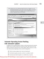
2. Choose Start | All Programs | Microsoft Office | Microsoft Office Tools | Microsoft Office
Application Recovery to display the Microsoft Office Application Recovery window:
3. Select the application that’s not responding.
4. Click the Recover Application button to try to recover the application.
5. If Microsoft Office Application Recovery is able to recover data, you’ll see a progress
report such as that shown below. The recovery operation may take anything from a few
seconds to several minutes, depending on how much data was involved.
6. Windows displays the error-reporting dialog box that invites you to send Microsoft a
report on the problem. If Microsoft Office Application Recovery may be able to save
some of your work, this dialog box includes an option for recovering your work and
restarting the application. Make sure this option is selected, then click the Send Error
Report button or the Don’t Send button as appropriate.
7. If the Recover Application option doesn’t work, click the End Application button to end
the application forcibly. (Clicking the End Application button has the same effect as
clicking the End Task button on the Applications tab of Windows Task Manager.)

78 How to Do Everything with Microsoft Office Excel 2003
HowTo-Tght (8) / How to Do Everything with Microsoft Office Excel 2003 / Hart-Davis / 3071-1 / Chapter 3
P:\010Comp\HowTo8\071-1\ch03.vp
Thursday, August 28, 2003 11:35:54 AM
Color profile: Generic CMYK printer profile
Composite Default screen
3
CHAPTER 3: Create Spreadsheets and Enter Data 79
HowTo-Tght (8) / How to Do Everything with Microsoft Office Excel 2003 / Hart-Davis / 3071-1 / Chapter 3
Recover a Workbook from an AutoRecover File
When an Office application restarts after a crash or after being closed by Microsoft Office
Application Recovery or Windows Task Manager, it displays the Document Recovery task pane
(shown below) on the left of the application window. The Document Recovery task pane lists any
files the application has recovered, together with original versions of the documents:
When you hover the mouse pointer over the entry for an available file in the Document
Recovery task pane, the application displays a drop-down button on the right side of the entry.
Click the button to display the menu, then choose Open, Save As, Delete (for AutoRecover
versions only, not for original files), or Show Repairs. Once you’ve opened a document, the
menu offers the choices View, Save As, Close, and Show Repairs.
The Show Repairs item displays the Repairs dialog box with a report showing which errors
(if any) were detected and repaired in the file. Figure 3-6 shows two examples of the Repairs
dialog box. In the first example, the news is good: Excel was able to repair the file. In the second
example, “damage to the file was so extensive that repairs were not possible” and “some data
may have been lost or corrupted.” Before you ask—yes, the workbook had lost a huge amount
of data, but some parts of it were recoverable.
After deciding which recovered file to keep, choose File | Save As to display the Save As
dialog box, and then save the file under a different name than the original file. This way, you’ll
P:\010Comp\HowTo8\071-1\ch03.vp
Thursday, August 28, 2003 11:35:55 AM
Color profile: Generic CMYK printer profile

Composite Default screen
be able to go back to the original file if you subsequently discover that the recovered file has
problems you didn’t identify when viewing it.
Click the Close button to close the Document Recovery task pane.
Approach the recovery of documents with as calm a mind as possible. Don’t fall sobbing
with relief on a recovered document and save it over your old document before making
sure it contains usable data without errors.
80 How to Do Everything with Microsoft Office Excel 2003
HowTo-Tght (8) / How to Do Everything with Microsoft Office Excel 2003 / Hart-Davis / 3071-1 / Chapter 3
FIGURE 3-6 The Repairs dialog box tells you whether Excel was able to repair the file or
whether data was lost.
P:\010Comp\HowTo8\071-1\ch03.vp
Thursday, August 28, 2003 11:35:55 AM
Color profile: Generic CMYK printer profile
Composite Default screen
HowTo-Tght (8) / How to Do Everything with Microsoft Office Excel 2003 / Hart-Davis / 3071-1 / Chapter 4
blind folio 81
Chapter 4
Format Worksheets
for Best Effect
P:\010Comp\HowTo8\071-1\ch04.vp
Thursday, August 28, 2003 11:42:38 AM
Color profile: Generic CMYK printer profile
Composite Default screen
82 How to Do Everything with Microsoft Office Excel 2003
HowTo-Tght (8) / How to Do Everything with Microsoft Office Excel 2003 / Hart-Davis / 3071-1 / Chapter 4
How to…
■
Add, delete, and manipulate worksheets
■

Format cells and ranges
■
Understand the number formats that Excel offers
■
Apply visual formatting to cells and ranges
■
Use conditional formatting to make remarkable values stand out
■
Apply canned formatting instantly with AutoFormat
■
Create and use styles to apply consistent formatting easily
A
s you saw in Chapter 3, Excel makes it easy to navigate in and enter data in worksheets.
Excel also offers a wide variety of formatting options for presenting the data in worksheets
as effectively as possible.
In this chapter, you’ll learn how to manipulate worksheets in a workbook before moving on
to discover how to format cells and ranges by using the many types of formatting that Excel supports.
Add, Delete, and Manipulate Worksheets
By default, each Excel workbook contains three worksheets and can contain from one to 255
worksheets. In the following sections, you’ll learn how to add, delete, hide, and redisplay worksheets;
move and copy worksheets; rename worksheets; and change the formatting on default new
worksheets that you create.
Add, Delete, Hide, and Redisplay Worksheets
You can add and delete worksheets to workbooks as follows:
■
To add a worksheet, select the worksheet before which you want the new worksheet
to appear, and choose Insert | Worksheet or press either
SHIFT-F11 or ALT-SHIFT-F1.
Alternatively, right-click the worksheet tab, choose Insert from the shortcut menu, select
Worksheet on the General tab of the Insert dialog box, and click the OK button.

You can change the default number of worksheets in a new workbook by adjusting the
value in the Sheets in New Workbook text box on the General tab of the Options dialog
box (Tools | Options).
■
To delete a worksheet, right-click its tab and choose Delete from the shortcut menu.
Alternatively, select the worksheet and choose Edit | Delete Sheet. Excel deletes the
worksheet without confirmation and doesn’t let you undo the deletion, so double-check
that you’ve picked the right worksheet before issuing the Delete command.
■
To hide a worksheet from view, select it and choose Format | Sheet | Hide. To display the
worksheet again, choose Format | Sheet | Unhide, select the sheet in the Unhide dialog
box, and click the OK button.
P:\010Comp\HowTo8\071-1\ch04.vp
Thursday, August 28, 2003 11:42:39 AM
Color profile: Generic CMYK printer profile
Composite Default screen
4
Move and Copy Worksheets
In a workbook that contains few worksheets, the easiest way to move a worksheet to a new position
in the workbook is to drag its tab to the new position. You can copy the worksheet instead of
moving it by holding down
CTRL as you drag. The copy receives the same name as the original
worksheet followed by the number two in parentheses.
In a workbook that contains many worksheets, it’s easier to use the Move or Copy dialog box
to move or copy a worksheet. Follow these steps:
1. Select the worksheet or worksheets that you want to move or copy.
2. Choose Edit | Move or Copy Sheet, or right-click a selected worksheet tab and choose
Move or Copy from the shortcut menu. Excel displays the Move or Copy dialog box:
3. Select the destination in the Before Sheet list box.
CHAPTER 4: Format Worksheets for Best Effect 83

HowTo-Tght (8) / How to Do Everything with Microsoft Office Excel 2003 / Hart-Davis / 3071-1 / Chapter 4
Recover from Deleting
the Wrong Worksheet
If you delete the wrong worksheet, the only way to recover your work is to revert to the
previously saved version of the workbook—if that version of the workbook contains the
worksheet. (If you’ve just inserted the worksheet in the workbook, entered data on it, and
deleted it, you’re stuck.)
To revert to the previously saved version of the workbook, close the workbook without
saving changes to it, and then open the workbook again.
When you close the workbook like this, you’ll also lose any other unsaved changes to the
workbook, so this isn’t an action to take lightly. But if the alternative is losing a worksheet
that contained valuable information, losing other unsaved changes may be worthwhile.
P:\010Comp\HowTo8\071-1\ch04.vp
Thursday, August 28, 2003 11:42:40 AM
Color profile: Generic CMYK printer profile
Composite Default screen
4. To copy the worksheet, select the Create a Copy check box.
5. Click the OK button to close the Move or Copy dialog box. Excel moves or copies the
worksheet.
The Move or Copy dialog box also enables you to move or copy a worksheet to a different
workbook. Open the workbook and follow the previous steps, but in the To Book drop-down list,
select the destination workbook.
When you copy a worksheet, Excel copies only the first 255 characters of each cell. If
any cell in the worksheet contains more than 255 characters, Excel warns you of this
problem, but it doesn’t specify the cells affected. To work around the problem, click the
Select All button to select the source worksheet, issue a Copy command, and then paste
the copies into the destination worksheet.
Rename a Worksheet
By default, Excel names worksheets Sheet1, Sheet2, and so on. You can rename worksheets
with new names of up to 31 characters. Usually, it’s best to keep worksheet names considerably

shorter than the maximum lengths so that there’s enough room for several tabs to appear at once
on an average-resolution screen.
To rename a worksheet, follow these steps:
1. Double-click the worksheet’s tab, or right-click the tab and choose Rename from the
shortcut menu. Excel selects the existing name.
2. Type the new name over or edit the existing name.
3. Press
ENTER or click elsewhere.
To make a worksheet tab easier to identify among its siblings, you can change its color.
Issue a Tab Color command from the Format | Sheet submenu or the tab’s shortcut
menu, select the color, and click the OK button.
84 How to Do Everything with Microsoft Office Excel 2003
HowTo-Tght (8) / How to Do Everything with Microsoft Office Excel 2003 / Hart-Davis / 3071-1 / Chapter 4
Change the Formatting on New
Default Worksheets and Workbooks
You can change the default formatting of the workbook and worksheets that Excel uses for
the New Blank Workbook command by creating a template named Book.xlt in the XLSTART
folder. This folder is located in your %userprofile%\Application Data\Microsoft\Excel\
folder (for example, C:\Documents and Settings\Jane Phillips\Application Data\Microsoft\
Excel\XLSTART).
P:\010Comp\HowTo8\071-1\ch04.vp
Thursday, August 28, 2003 11:42:40 AM
Color profile: Generic CMYK printer profile
Composite Default screen
4
Format Cells and Ranges
As you’ve seen already in this book, the cell is the basis of the Excel worksheet. A cell can
contain any one of various types of data—numbers (values that can be calculated), dates, times,
formulas, text, etc.—and can be formatted in a variety of ways. You can adjust everything from
the formats in which Excel displays different types of data to alignment to background color and

gridlines.
The most basic type of formatting controls the way in which Excel displays the data the cell
contains. For some types of entries, Excel displays the literal contents of the cell by default; for other
types of entries, Excel displays the results of the cell’s contents. For example, when you enter a
formula in a cell, by default, Excel displays the results of the formula rather than the formula itself.
So to be sure of the contents of a cell, you need to make it the active cell or edit it. Excel displays the
literal contents of the active cell in the Formula bar; and, when you edit a cell, Excel displays its literal
contents in both the cell itself and in the Formula bar.
Even when Excel displays the contents of the cell, it may change the contents for display
purposes. For example, when you enter a number that’s too long to be displayed in a General-
formatted cell, Excel converts it to scientific notation using six digits of precision. Similarly,
Excel rounds display numbers when they won’t fit in cells, but the underlying number remains
unaffected.
CHAPTER 4: Format Worksheets for Best Effect 85
HowTo-Tght (8) / How to Do Everything with Microsoft Office Excel 2003 / Hart-Davis / 3071-1 / Chapter 4
Before you can navigate to the XLSTART folder, you’ll need to display hidden files and
folders (if you haven’t already done so). Choose Tools | Options in an Explorer window to
display the Folder Options dialog box, select the Show Hidden Files and Folders option on
the View tab, and click the OK button.
Then open an Explorer window to the XLSTART folder and take either of the following
actions:
■
If you have a workbook or template that contains the formatting that you want to use
for new default worksheets and workbooks, copy it to the XLSTART folder. Press
F2 and rename the copy Book.xlt. (If the file was a workbook, Windows displays a
Rename dialog box that warns you about the change of file extension. Click the Yes
button.) Open Book.xlt and delete any contents you don’t want to have in the new
default worksheets and workbooks. Save and close the file.
■
If you don’t have a workbook or template that contains the formatting you want to

use for new default worksheets and workbooks, create a new one. In the XLSTART
folder, issue a New | Microsoft Excel Worksheet command from the File menu or
context menu. Name the new workbook Book.xlt. Windows displays a Rename
dialog box that warns you about the change of file extension. Click the Yes button.
Open Book.xlt, set it up with the formatting you want to use for new default
worksheets and workbooks, save it, and close it.
P:\010Comp\HowTo8\071-1\ch04.vp
Thursday, August 28, 2003 11:42:41 AM
Color profile: Generic CMYK printer profile
Composite Default screen
Apply Number Formatting
The main way of applying formatting to cells and ranges is the Format Cells dialog box (Format |
Cells). You can also apply basic formatting from the Formatting toolbar, shown here with labels.
(If the Formatting toolbar isn’t currently displayed, right-click the menu bar or any displayed
toolbar and choose the Formatting entry to display it.)
If you find the Formatting toolbar to be a more convenient way to apply formatting than
the Format Cells dialog box, customize the Formatting toolbar by adding to it buttons
for the types of formatting you apply most frequently. You’ll find a few extra buttons on
the Add or Remove Buttons | Formatting submenu. You’ll find all of the formatting
commands under the Format category on the Commands tab of the Customize dialog
box. Chapter 17 explains how to customize toolbars and menus.
Excel’s Format Cells dialog box (choose Format | Cells or press
CTRL-1) offers a large
number of options for formatting the active cell or selected ranges. You’ll learn about most of
these options later in this chapter. (Other options, such as those for locking and protecting cells,
you’ll learn about later in this book.)
You can also apply some font formatting via standard Office shortcuts (such as
CTRL-B for
boldface,
CTRL-I for italic, and CTRL-U for single underline).

Understand Excel’s Number Formats
To make Excel display the contents of a cell in the way you intend, apply the appropriate number
format. You can apply number formats manually in several ways, but Excel also applies number
formats automatically when you enter text that matches one of Excel’s triggers for a number format.
Because some of the triggers for automatic number formatting are less than intuitive, it’s a good idea
to know about them so that you can avoid having Excel apply the number formats unexpectedly.
The central place for applying number formats is the Number tab of the Format Cells dialog
box (Figure 4-1). The Number tab offers 12 categories of built-in formats. The following sections
discuss these formats.
86 How to Do Everything with Microsoft Office Excel 2003
HowTo-Tght (8) / How to Do Everything with Microsoft Office Excel 2003 / Hart-Davis / 3071-1 / Chapter 4
Bold
Underline
Center
Merge and Center
Percent Style
Increase Decimal
Decrease Indent
Font Size
Italic
Align Left
Font
Align Right
Currency Style
Comma Style
Decrease Decimal
Increase Indent
Fill Color
Font Color
Borders

P:\010Comp\HowTo8\071-1\ch04.vp
Thursday, August 28, 2003 11:42:41 AM
Color profile: Generic CMYK printer profile
Composite Default screen
4
CHAPTER 4: Format Worksheets for Best Effect 87
HowTo-Tght (8) / How to Do Everything with Microsoft Office Excel 2003 / Hart-Davis / 3071-1 / Chapter 4
General Number Format
The General number is the default format for all cells on a new worksheet (unless you’ve
customized it). General displays up to 11 digits per cell and doesn’t use thousands separators.
You can apply General format by pressing
CTRL-SHIFT-~ (tilde).
Number Format
The Number formats let you specify the number of decimal places to display (0 to 30, with a
default of 2), whether to display a thousands separator (for example, a comma in U.S. English
formats), and how to represent negative numbers.
You can make Excel apply the Number format with the thousands separator by including a
comma to separate thousands or millions (for example, enter 1,000, 1,000,000,or1,000000—only
one appropriately placed comma is necessary).
Currency Format
The Currency formats let you specify the number of decimal places to display (0 to 30, with a
default of 2), which currency symbol to display (if any), and how to represent negative numbers.
You can make Excel apply Currency format by entering the appropriate currency symbol
before the number. For example, enter $4 to make Excel display dollar formatting. If you enter
one or more decimal places, Excel applies Currency format with two decimal places. For example,
if you enter $4.1, Excel displays $4.10.
FIGURE 4-1 Use the options on the Number tab of the Format Cells dialog box to apply
number formatting.
P:\010Comp\HowTo8\071-1\ch04.vp
Thursday, August 28, 2003 11:42:42 AM

Color profile: Generic CMYK printer profile
Composite Default screen
Accounting Format
The Accounting formats let you specify the number of decimal places to display (0 to 30, with a
default of 2) and which currency symbol to display (if any). The currency symbol appears flush
left with the cell border, separated from the figures. The Accounting formats represent negative
numbers with parentheses around them—there’s no choice of format.
You can apply the Accounting format quickly by clicking the Currency Style button on the
Formatting toolbar.
Date Format
The Date formats offer a variety of date formats based on the locale you choose. These options
are easy to understand. What’s more important to grasp is how Excel stores dates and times.
Excel treats dates and times as serial numbers representing the number of days that have
elapsed since 1/1/1900, which is given the serial number 1. For example, the serial date 37955
represents November 30, 2003.
Excel for the Macintosh uses a different starting date—January 2, 1904—instead of
January 1, 1900. If you use spreadsheets created in Excel for the Mac in Windows
versions of Excel, you’ll need to select the 1904 Date System check box in the Workbook
Options section of the Calculation tab of the Options dialog box to get Excel to display
the dates correctly.
For computers, serial dates (and times) are a snap to sort and manipulate: to find out how far
apart two dates are, the computer need merely subtract one date from the other, without having to
consider which months are shorter than others or whether a leap year is involved. For humans,
serial dates are largely inscrutable, so Excel displays dates in your choice of format.
If you want, you can enter dates by formatting cells with the Date format and entering the
appropriate serial number, but most people find it far easier to enter the date in one of the conventional
Windows formats that Excel recognizes. Excel automatically converts to serial dates and formats
with a Date format any entry that contains a hyphen (-) or a forward slash (/) and matches one of
the date and time formats Windows uses. For example, if you enter 11/30/04, Excel assumes you
mean November 30, 2004.

If you don’t specify the year, Excel assumes you mean the current year
Time Format
The Time formats offer a variety of time formats based on 12-hour and 24-hour clocks. These
options are easy to understand. Excel treats times as subdivisions of days, with 24 hours making
up one day and one serial number. So, given that 37987 is the serial date for January 1, 2004,
37987.5 is noon on that day, 37987.25 is 6
AM, 37987.75 is 6PM, and so on.
You can make Excel automatically format an entry with a time format by entering a number
that contains a colon (for example, 12:00) or a number followed by a space and an uppercase or
lowercase a or p (for example, 1 P or 11 a).
88 How to Do Everything with Microsoft Office Excel 2003
HowTo-Tght (8) / How to Do Everything with Microsoft Office Excel 2003 / Hart-Davis / 3071-1 / Chapter 4
P:\010Comp\HowTo8\071-1\ch04.vp
Thursday, August 28, 2003 11:42:42 AM
Color profile: Generic CMYK printer profile
Composite Default screen
4
Percentage Format
The Percentage format displays the value in the cell with a percent sign and with your choice of
number of decimal places (the default is two). For example, if you enter 71 in the cell, Excel
displays 71.00% by default.
You can make Excel automatically format an entry with the Percentage format by entering a
percent sign after the number. If you enter no decimal places, Excel uses none. If you enter one
or more decimal places, Excel uses two decimal places. You can change the number of decimal
places displayed by formatting the cell manually.
Fraction Format
Excel stores fractions as their decimal equivalents—for example, it stores ¼ as 0.25. To display
fractions (for example, ¼) and compound fractions (for example, 11¼) in Excel, you have to use
the Fraction formats. Excel offers fraction formats of one digit (for example, ¾), two digits (for
example,

16
/18), and three digits (for example,
303
/512)—halves, quarters, eighths, sixteenths, tenths,
and hundreds.
Before worrying about fractions being displayed as their decimal equivalents, however, you
need to worry about entering many fractions in a way that Excel won’t mistake for dates. For
example, if you enter 1/4 in a General-formatted cell, Excel converts it to the date 4-Jan in the
current year.
To enter a fraction in a General-formatted cell, type a zero, a space, and the fraction—for
example, type 0 1/4 to enter ¼. To enter a compound fraction in a General-formatted cell, type
the integer, a space, and the fraction—for example, type 11 1/4 to enter 11¼. Excel formats the
cell with the appropriate Fraction format, so the fraction is displayed, and stores the corresponding
decimal value.
If you need to enter simple fractions consistently in your worksheets, format the relevant
cells, columns, or rows with the Fraction format ahead of time.
Scientific Format
Scientific format displays numbers in an exponential form—for example, 567890123245 is
displayed as 5.6789E+11, indicating where the decimal place needs to go. You can change the
number of decimal places displayed to anywhere from 0 to 30.
You can make Excel apply Scientific format by entering a number that contains an e in any
position but the ends (for example, 3e4 or 12345E17).
Text Format
Text format is for values that you want to force Excel to treat as text so as to avoid having Excel
automatically apply another format. For example, if you keep a spreadsheet of telephone numbers,
you might have some numbers that start with 0. To prevent Excel from dropping what appears to
be a leading zero and converting the cell to a number format, you could format the cell as Text.
(You could also use the Special format for phone numbers, discussed in the next section.)
HowTo-Tght (8) / How to Do Everything with Microsoft Office Excel 2003 / Hart-Davis / 3071-1 / Chapter 4
CHAPTER 4: Format Worksheets for Best Effect 89

P:\010Comp\HowTo8\071-1\ch04.vp
Thursday, August 28, 2003 11:42:42 AM
Color profile: Generic CMYK printer profile
Composite Default screen
Similarly, you might need to enter a value that Excel might take to be a date (for example, 1/2), a
time, a formula, or another format.
Excel left-aligns Text-formatted entries and omits them from range calculations—for example,
SUM()—in which they would otherwise be included.
You can make Excel format a numeric entry with the Text format by entering a space before
the number.
For safety, force the Text format by typing a space before a numeric entry or manually
format the cell as Text before entering data in it. If you apply the Text format to numbers
you’ve already entered, Excel will continue to treat them as numbers rather than as text.
You’ll need to edit each cell (double-click it, or press
F2, and then press ENTER to accept
the existing entry) to correct this error.
Special Format
The Special formats provide a locale-specific range of formatting choices. For example, the
English (United States) locale offers the choices Zip Code, Zip Code + 4, Phone Number, and
Social Security Number.
As you’ll quickly realize, these formats all have rigidly defined formats, most of which are
separated by hyphens into groups of specific lengths. (Phone numbers are less rigid than the
other formats, but Excel handles longer numbers—for example, international numbers—as well
as could be expected.)
Special formats enable you to quickly enter numbers of the given type and have Excel enter
the hyphens automatically for you. For example, if you format a cell with the Social Security
Number format and enter 623648267, Excel automatically formats it as 623-64-8267.
Custom Format
The Custom format enables you to define your own custom formats for needs that none of the
built-in formats covers.

Excel includes a variety of built-in formats that cover general, numeric, currency, percentage,
exponential, date, time, and custom numeric formats. You can also design your own custom
formats based on one of the built-in formats.
To define a custom format, follow these steps:
1. Enter sample text for the format in a cell, and then select that cell. (Excel then displays
the sample text in the format you’re creating, which helps you see the effects of your
changes.)
2. Display the Number tab of the Format Cells dialog box.
3. In the Category box, select the Custom item.
4. In the Type list box, select the custom format on which you want to base your new
custom format. Excel displays the details for the type in the Type text box.
90 How to Do Everything with Microsoft Office Excel 2003
HowTo-Tght (8) / How to Do Everything with Microsoft Office Excel 2003 / Hart-Davis / 3071-1 / Chapter 4
P:\010Comp\HowTo8\071-1\ch04.vp
Thursday, August 28, 2003 11:42:43 AM
Color profile: Generic CMYK printer profile
Composite Default screen
4
5. If the details for the type extend beyond the Type text box, double-click in the Type text
box to select all of its contents, issue a Copy command (for example, press
CTRL-C), and
then paste the copied text into a text editor, such as Notepad. (For a shorter type, you can
work effectively in the Type text box. For a longer type, it’s easier to have enough space
to see the whole type at once.)
6. Enter the details for the four parts of the type, separating the parts from each other with a
semicolon. (See the detailed explanation below.)
7. If you’re working in a text editor, copy what you typed and paste it into the Type text
box. Check the sample text to make sure it seems to be correct.
8. Click the OK button.
Each custom format consists of format codes that specify how Excel should display the

information. Each custom format can contain four formats. The first format specifies how to
display positive numbers, the second format specifies how to display negative numbers, the third
format specifies how to display zero values, and the fourth format specifies how to display text.
The four formats are separated by semicolons. You can leave a section blank by entering nothing
between the relevant semicolons (or before the first semicolon, or after the last semicolon).
Table 4-1 explains the codes you can use for defining custom formats.
CHAPTER 4: Format Worksheets for Best Effect 91
HowTo-Tght (8) / How to Do Everything with Microsoft Office Excel 2003 / Hart-Davis / 3071-1 / Chapter 4
Code Meaning Example
[color name] Display the specified color. Enter the appropriate color in brackets as the first item
in the section: [Black], [Red], [Blue], [Green], [White],
[Cyan], [Magenta], or [Yellow].
For example, #,##0_);[Magenta](#,##0) displays
negative numbers in magenta.
Number Format Codes
# Display a significant digit. ##.# displays two significant digits before the decimal
point and one significant digit after it. (A significant
digit is a nonzero figure.)
0 Display a zero if there would
otherwise be no digit in this
place.
00000 displays a five-digit number, packing it with
leading zeroes if necessary. For example, if you enter 4,
Excel displays 00004.
% Display a percentage. #% displays the number multiplied by 100 and with a
percent sign. For example, 2 appears as 200%.
? Display as a fraction. # ????/???? displays a number and four-digit
fractions—for example, 4 1234/4321.
. Display a decimal point. ##.## displays two significant digits on either side of
the decimal point.

TABLE 4-1 Codes for Creating Custom Formats
P:\010Comp\HowTo8\071-1\ch04.vp
Thursday, August 28, 2003 11:42:43 AM
Color profile: Generic CMYK printer profile
Composite Default screen
92 How to Do Everything with Microsoft Office Excel 2003
HowTo-Tght (8) / How to Do Everything with Microsoft Office Excel 2003 / Hart-Davis / 3071-1 / Chapter 4
Code Meaning Example
, Two meanings: Display the
thousands separator or scale
the number down by 1,000.
Thousands separator example: $#,### displays the
dollar sign, four significant digits, and the thousands
separator.
Scale by 1,000 example: €#.##,,, " billion" displays the
euro symbol, one significant digit before the decimal
point and two after, the number scaled down by a
billion, and the word billion (after a space). For
example, if you enter 9876543210, Excel displays
€ 9.88 billion.
Date and Time Format Codes
d Display the day in numeric
format.
d-mmm-yyyy displays 1/1/04 as 1-Jan-2004.
dd Display the day in numeric
format with a leading zero.
dd/mmm/yy displays 1/1/04 as 01/Jan/04. Use leading
zeroes to align dates.
ddd Display the day as a
three-letter abbreviation.

ddd dd/mm/yyyy displays 1/1/04 as Thu 01/01/2004.
dddd Display the day in full. dddd, dd/mm/yyyy displays 1/1/04 as Thursday,
01/01/2004.
m Display the month in
numeric format.
d/m/yy displays 1/1/04 as 1/1/04.
mm Display the month in
numeric format with a
leading zero.
dd/mm/yy displays 1/1/04 as 01/01/04.
mmm Display the month as a
three-letter abbreviation.
dd-mmm-yy displays 1/1/04 as 01-Jan-2004.
mmmm Display the month in full. d mmmm, yyyy displays 1/1/04 as 1 January, 2004.
mmmmm Display the month as a
one-letter abbreviation.
January, June, and July appear as J; April and August
appear as A; and so on. This code is seldom useful
because it tends to be visually confusing.
yy Display the year as a
two-digit number.
d/m/yy displays 1/1/04 as 1/1/04.
yyyy Display the year in full. d-mmm-yyyy displays 1/1/04 as 1-Jan-2004.
h Display the hour. h:m displays 1:01 as 1:1.
hh Display the hour with a
leading zero.
hh:mm displays 1:01 as 01:01.
m Display the minute. h:m displays 1:01 as 1:1.
mm Display the minute with a
leading zero.

hh:mm displays 1:01 as 01:01. To distinguish mm from
the months code, you must enter it immediately after hh
or immediately before ss.
TABLE 4-1 Codes for Creating Custom Formats (continued)
P:\010Comp\HowTo8\071-1\ch04.vp
Thursday, August 28, 2003 11:42:44 AM
Color profile: Generic CMYK printer profile
Composite Default screen
4
Apply Visual Formatting
After specifying how Excel should represent the data you enter in worksheet cells, you’ll probably
want to apply formatting to the worksheets to make them more readable. Excel offers a wide range
of formatting options, most of which are easy to understand and applicable to a cell or range.
The following list outlines the main types of formatting that Excel offers. The primary way
of applying these formatting options is the Format Cells dialog box (choose Format | Cells or
CHAPTER 4: Format Worksheets for Best Effect 93
HowTo-Tght (8) / How to Do Everything with Microsoft Office Excel 2003 / Hart-Davis / 3071-1 / Chapter 4
Code Meaning Example
s Display the second. h:m:s displays 1:01:01 as 1:1:1.
ss Display the second with a
leading zero.
hh:mm:ss displays 1:01:01 as 1:01:01.
.0, .00, .000 Display tenths, hundredths,
or thousandths of seconds.
h:mm:ss.00 displays 1:01:01.11 as 1:01:01.11. Use
further zeroes for greater precision.
A/P Display A for
A.M. and P
for
P. M.

h:mm A/P displays 1:01 as 1:01 A. You can use
uppercase A/P or lowercase a/p to specify which
case to display.
AM/PM Display AM for
A.M. and PM
for
P. M.
h:mm am/pm displays 13:01 as 1:01 PM. Excel uses
uppercase regardless of which case you use.
[] Display the elapsed time in
the specified unit.
[h]:mm:ss displays the elapsed time in hours, minutes,
and seconds—for example, 33:22:01.
Text Format Codes
_ Display a space as wide as
the specified character.
_) makes Excel enter a space the width of a closing
parenthesis—for example, to align positive numbers
with negative numbers surrounded by parentheses.
* Repeat the specified
character to fill the cell.
*A makes Excel fill the cell with A characters.
Sometimes useful for drawing attention to particular
values—for example, zero values.
\ Display the following
character.
[Blue]$#,###.00 \*;[Red]$#,###.00 \D displays positive
numbers in blue and followed by an asterisk, and
negative numbers in red and followed by a D.
"string" Display the string of text. $#,##0.00" Advance" displays the word Advance

after the entry. Note the leading space between the "
and the word.
@ Concatenate the specified
string with the user’s text
input.
“Username: “@ enters Username: and a space before
the user’s text input. This works only in the fourth
section (the text section) of a custom format.
N/A Display the specified
character.
$ - + = / ( ) { } : ! ^ & ‘ ’ ~ < > [SPACE]
TABLE 4-1 Codes for Creating Custom Formats (continued)
P:\010Comp\HowTo8\071-1\ch04.vp
Thursday, August 28, 2003 11:42:44 AM
Color profile: Generic CMYK printer profile
Composite Default screen
press CTRL-1). You can also apply basic formatting by using the buttons on the Formatting
toolbar.
■
Font formatting Change fonts, font size, font style (regular, bold, italic, or bold italic),
underline, and color. When you change the formatting, Excel clears the Normal Font
check box. Reselect this option to reapply the normal font—in other words, remove all
of the font formatting that you’ve applied to the selection. These options appear on the
Font tab of the Format Cells dialog box (shown on the left in Figure 4-2).
■
Alignment formatting Change cells’ horizontal and vertical alignment. Options
include horizontal centering across the selection (which can be useful for centering a
heading over several columns), vertical centering in a cell whose height you’ve
increased, and indentation. These options appear on the Alignment tab of the Format
Cells dialog box (shown on the right in Figure 4-2).

■
Orientation and text-direction formatting Specify the orientation of the text—for
example, set text at a slant for special emphasis, or create a vertical heading to save
space. Specify the direction of the text: Left-to-Right, Right-to-Left, or Context (Excel
decides based on the context). These options appear on the Alignment tab of the Format
Cells dialog box.
■
Text-control formatting Choose whether to wrap text in the cell, shrink it to fit the
cell, or merge multiple cells into one cell. Wrapping text can greatly improve long
94 How to Do Everything with Microsoft Office Excel 2003
HowTo-Tght (8) / How to Do Everything with Microsoft Office Excel 2003 / Hart-Davis / 3071-1 / Chapter 4
FIGURE 4-2 Use the Font tab (left) of the Format Cells dialog box to apply font formatting
and the Alignment tab (right) to control alignment, text orientation, and text
direction.
P:\010Comp\HowTo8\071-1\ch04.vp
Thursday, August 28, 2003 11:42:45 AM
Color profile: Generic CMYK printer profile
Composite Default screen