how to do everything with ms office excel 2003 phần 5 ppsx

Here are three examples of using the date and time functions:
■
=TODAY() enters the current date in a cell, and =NOW() enters the current date and
time, in an automatically updating form.
■
=DATEVALUE("2004-4-1") converts the text string “2004-4-1” to its corresponding serial
date. By default, Excel displays the result with Date formatting, but you can apply other cell
formatting (for example, you might choose to display the serial number for the date).
■
=HOUR("11:45 PM") returns 23, the hour derived from 11:45 P.M.
Financial Functions
Excel includes 16 financial functions, explained in Table 7-2, for common calculations, and the
Analysis ToolPak (one of Excel’s add-ins that you can load by choosing Tools | Add-Ins) adds
about three dozen extra financial functions for more arcane calculations.
158 How to Do Everything with Microsoft Office Excel 2003
HowTo-Tght (8) / How to Do Everything with Microsoft Office Excel 2003 / Hart-Davis / 3071-1 / Chapter 7
Function What It Returns
TODAY Current date, formatted as a date
NOW Current date and time, formatted as a date and time
WEEKDAY Weekday for the specified day, as a serial number between 1 (Sunday) and 7
(Saturday)
TABLE 7-1 Excel’s Date and Time Functions (continued)
Function What It Returns
DB Depreciation using the fixed-declining balance method
DDB Depreciation using the double-declining balance method or other method
FV Future value of an investment
IPMT Interest payments for an investment for a specified period
IRR Internal rate of return for cash flows
MIRR Modified internal rate of return for cash flows
ISPMT Interest paid for an investment over a specified period
NPER Number of periods for an investment

NPV Net present value of an investment
PMT Payment for a loan
PPMT Payment on the principal for an investment
PV Present value of an investment
TABLE 7-2 Excel’s Financial Functions
P:\010Comp\HowTo8\071-1\ch07.vp
Thursday, August 28, 2003 11:56:57 AM
Color profile: Generic CMYK printer profile
Composite Default screen
7
Here are two examples of using the financial functions:
■
=PMT(7.25%/12,24,-20000) calculates the payment required to pay off a $20,000 loan
at 7.25% APR over 24 payments.
■
=DB(15000,3000,6,3) calculates the depreciation over the third year of an asset with an initial
cost of $15,000, a salvage value of $3,000 at the end of its life, and a life of six years.
Logical Functions
Excel’s six logical functions, explained in Table 7-3, enable you to test logical conditions. By
combining these logical functions with other functions, you can make Excel take action that’s
appropriate to how the condition evaluates.
Here are two examples of using the logical functions:
■
=IF(C21>4000,"More than $4,000","$4,000 or less") returns More than $4,000 if C21
contains a number greater than 4000. Otherwise, the function returns $4,000 or less.
■
=AND(INFO("system")="pcdos",INFO("osversion")="Windows (32-bit) NT
5.01",INFO("release")="11.0") returns TRUE if the user is running Excel 2003
(version 11.0) on Windows XP (aka Windows [32-bit] NT 5.01) on a PC.
HowTo-Tght (8) / How to Do Everything with Microsoft Office Excel 2003 / Hart-Davis / 3071-1 / Chapter 7

CHAPTER 7: Perform Calculations with Functions 159
Function What It Returns
RATE Interest rate per period of an investment
SLN Straight-line depreciation for an asset
SYD Sum-of-years’ digits depreciation for an asset
VDB Depreciation for an asset using the double-declining balance method or a variable
declining balance
TABLE 7-2 Excel’s Financial Functions (continued)
Function What It Returns
AND TRUE if all the specified arguments are TRUE; otherwise FALSE
FALSE FALSE (always—use to generate a FALSE value)
IF The first specified value if the condition is TRUE; the second specified value if the
condition is FALSE. (See the first example above.)
NOT FALSE from TRUE; TRUE from FALSE
OR TRUE if any of the specified arguments is TRUE; FALSE if all arguments are FALSE
TRUE TRUE (always—use to generate a TRUE value)
TABLE 7-3 Excel’s Logical Functions
P:\010Comp\HowTo8\071-1\ch07.vp
Thursday, August 28, 2003 11:56:57 AM
Color profile: Generic CMYK printer profile
Composite Default screen
Often IF is used with the information functions discussed in the next section, which contains
further examples.
Information Functions
Excel offers 16 information functions, explained in Table 7-4, for returning information about the
contents and formatting of the current cell or range. Some of these information functions are
widely useful, whereas others are more specialized.
Here are three examples of using the information functions:
■
=INFO("osversion") returns Windows’ internal description of the operating system

version—for example, Windows (32-bit) NT 5.01 for Windows XP. =INFO("directory")
returns the current working directory. =INFO("numfile") returns the number of active
worksheets in all open workbooks.
160 How to Do Everything with Microsoft Office Excel 2003
HowTo-Tght (8) / How to Do Everything with Microsoft Office Excel 2003 / Hart-Davis / 3071-1 / Chapter 7
Function What It Returns
CELL Specified details of the contents, location, or formatting of the first cell in the
specified range.
COUNTBLANK Number of empty cells in the specified range.
ERROR.TYPE A number representing the error value in the cell: 1 for #NULL!, 2 for #DIV/0!, 3
for #VALUE!, 4 for #REF!, 5 for #NAME?, 6 for #NUM!, and 7 for #N/A.
INFO Information about Excel, the operating system, or the computer.
ISBLANK TRUE if the cell is blank; FALSE if it has contents.
ISERR TRUE if the cell contains any error except #N/A; otherwise FALSE.
ISERROR TRUE if the cell contains any error; otherwise FALSE.
ISLOGICAL TRUE if the cell contains a logical value; otherwise FALSE.
ISNA TRUE if the cell contains #N/A; otherwise FALSE.
ISNONTEXT TRUE if the cell contains anything but text—even if it’s a blank cell; otherwise FALSE.
ISNUMBER TRUE if the cell contains a number; otherwise FALSE.
ISREF TRUE if the cell contains a reference; otherwise FALSE.
ISTEXT TRUE if the cell contains text; otherwise FALSE.
N A number derived from the specified value: a number returns that number, a date
returns the associated serial date, TRUE returns 1, FALSE returns 0, an error returns
its error value (see the ERROR.TYPE entry, earlier in this table), and anything else
returns 0.
NA #N/A (used to enter the error value deliberately in the cell).
TYPE A number representing the data type in the cell: 1 for a number, 2 for text, 4 for a
logical value, 16 for an error value, and 64 for an array.
TABLE 7-4 Excel’s Information Functions
P:\010Comp\HowTo8\071-1\ch07.vp

Thursday, August 28, 2003 11:56:57 AM
Color profile: Generic CMYK printer profile
Composite Default screen
7
■
=IF(ISERROR(Revenue/Price), "Units not available", Revenue/Price) checks to see
whether dividing the cell referenced by the name Revenue by the cell referenced by the
name Price will result in an error before it performs the calculation. If the calculation
will result in an error, the formula displays a label in the cell instead. If the calculation
won’t result in an error, the formula performs the calculation and displays its result.
■
=IF(ISBLANK('Amortization Estimates.xls'!Amortization_Rate), "Warning: Base
rate not entered","") displays a warning message if the Amortization_Rate cell in the
Amortization Estimates workbook is blank. Otherwise, the formula displays nothing.
The Analysis ToolPak also contains the ISEVEN function, which returns TRUE if the
specified number is even, and the ISODD function, which returns TRUE if the specified
number is odd.
Lookup and Reference Functions
Excel includes 18 lookup and reference functions for returning information from lists and tables.
You’ll see some of these functions in action in Chapter 9, which discusses how to create
databases and lists in Excel.
Mathematical and Trigonometric Functions
Excel offers 50 mathematical and trigonometric functions (and the Analysis ToolPak offers about
10 more). Many of these functions are self-explanatory to anyone who needs to use them in their
work. For example, COS returns the cosine of an angle, COSH returns the hyperbolic cosine,
ACOS returns the arccosine, and ACOSH returns the inverse hyperbolic cosine. Table 7-5
explains the mathematical and trigonometric functions you might use occasionally for more
general purposes.
Here are three examples of using the general-purpose mathematical and trigonometric functions:
■

=SUM(A1:A24) adds the values in the range A1:A24.
■
=RAND() enters a random value that changes each time the worksheet is recalculated.
(Unless you turn off automatic calculation, Excel recalculates the worksheet each time
you enter a change.)
■
=ROMAN(1998) returns MCMXCVIII.
Statistical Functions
Excel includes a large number of statistical functions that fall into categories such as calculating
deviation (including AVEDEV, STDEVA, STDEV, and STDEVP), distributions (BETADIST,
CHIDIST, BINOMDIST, EXPONDIST, KURT, POISSON, and WEIBULL), and transformations
(FISHER and FISHERINV).
CHAPTER 7: Perform Calculations with Functions 161
HowTo-Tght (8) / How to Do Everything with Microsoft Office Excel 2003 / Hart-Davis / 3071-1 / Chapter 7
P:\010Comp\HowTo8\071-1\ch07.vp
Thursday, August 28, 2003 11:56:58 AM
Color profile: Generic CMYK printer profile
Composite Default screen
Unless you’re working with statistics, you’re unlikely to need most of the statistical
functions. However, you may need to use some of these functions for more general business
purposes; these general statistical functions are listed in Table 7-6.
Here are three examples of using the general-purpose statistical functions:
■
=AVERAGE(Q1Sales) returns the average value of the entries in the range named
Q1Sales.
■
=COUNTBLANK(BA1:BZ256) returns the number of blank cells in the
specified range.
■
=COUNTIF(Q2Sales,0) returns the number of cells with a zero value in the range

named Q2Sales.
Text Functions
Excel contains 24 functions for manipulating text, explained in Table 7-7. One of them,
BAHTTEXT, is highly esoteric, and another, CONCATENATE, is seldom worth using because
the & operator is usually easier for concatenating text strings. You may find the other text
functions useful when you need to return a specific part (for example, the first five characters)
of a text string, change the case of a text string, or find one string within another string.
162 How to Do Everything with Microsoft Office Excel 2003
HowTo-Tght (8) / How to Do Everything with Microsoft Office Excel 2003 / Hart-Davis / 3071-1 / Chapter 7
Function What It Returns
ABS Absolute value (without the sign) of the specified number
EVEN Specified positive number rounded up to the next even integer, or the specified
negative number rounded down to the next even integer
ODD Specified positive number rounded up to the next odd integer, or the specified
negative number rounded down to the next odd integer
INT Specified number rounded down to the nearest integer
MOD Remainder left over after a division operation
RAND Random number (greater than or equal to 0 and less than 1)
ROMAN Roman equivalent of the specified Arabic numeral
ROUND Specified number rounded to the specified number of digits
ROUNDDOWN Specified number rounded down to the specified number of digits
ROUNDUP Specified number rounded up to the specified number of digits
SIGN 1 for a positive number, 0 for 0, and –1 for a negative number
SUM Total of the numbers in the specified range
SUMIF Total of the numbers in the cells in the specified range that meet the criteria given
TRUNC Specified number truncated to the specified number of decimal places
TABLE 7-5 Excel’s General-Purpose Mathematical and Trigonometric Functions
P:\010Comp\HowTo8\071-1\ch07.vp
Thursday, August 28, 2003 11:56:58 AM
Color profile: Generic CMYK printer profile

Composite Default screen
7
CHAPTER 7: Perform Calculations with Functions 163
HowTo-Tght (8) / How to Do Everything with Microsoft Office Excel 2003 / Hart-Davis / 3071-1 / Chapter 7
Function What It Returns
AVERAGE Average of the specified cells, ranges, or arrays
MEDIAN Median (the number in the middle of the given set) of the numbers in the
specified cells
MODE Value that occurs most frequently in the specified range of cells
COUNT Number of cells in the specified range that either contain numbers or include
numbers in their list of arguments
COUNTBLANK Number of empty cells in the specified range
COUNTIF Number of cells in the specified range that meet the specified criteria
MAX Largest value in the specified range
MIN Lowest value in the specified range
TABLE 7-6 Excel’s General-Purpose Statistical Functions
Function What It Returns
BAHTTEXT Number converted to Thai text and with the Baht suffix
CHAR Character represented by the specified character code
CODE Character code for the first character in the specified string
CLEAN Specified text string with all nonprintable characters stripped out (sometimes
useful when importing files in other formats)
CONCATENATE Text string consisting of the specified text strings joined together
DOLLAR Specified number converted to text in the Currency format
EXACT TRUE if the specified two text strings contain the same characters in the same
case; otherwise FALSE
FIND Starting position of one specified text string within another text
string—case-sensitive
FIXED Specified number rounded to the specified number of decimals, with or without
commas

LEN Number of characters in the specified text string
LEFT Specified number of characters from the beginning of the specified text string
RIGHT Specified number of characters from the end of the specified text string
MID Specified number of characters after the specified starting point in the specified
text string
LOWER Text string converted to lowercase
UPPER Text string converted to uppercase
TABLE 7-7 Excel’s Text Functions
P:\010Comp\HowTo8\071-1\ch07.vp
Thursday, August 28, 2003 11:56:58 AM
Color profile: Generic CMYK printer profile
Composite Default screen
Here are three examples of using the text functions:
■
=EXACT(A1,A2) compares the text in cells A1 and A2, returning TRUE if they’re
exactly alike (including case) and FALSE if they’re not.
■
=IF(LEN(H2)>=5, LEFT(H2,5),H2) returns the first five characters of cell H2 if the
length of the cell’s contents is five characters or more. If the length is less than five, the
formula returns the full contents of the cell.
■
=TRIM(CLEAN(C2)) strips nonprintable characters from the text string in cell C2,
removes extra spaces, and returns the resulting text string.
164 How to Do Everything with Microsoft Office Excel 2003
HowTo-Tght (8) / How to Do Everything with Microsoft Office Excel 2003 / Hart-Davis / 3071-1 / Chapter 7
Function What It Returns
PROPER Text string converted to “proper case” (first letter capitalized, the rest lowercase)
REPLACE Specified text string with the specified replacement string inserted in a specified
location
REPT Specified text string repeated the specified number of times

SEARCH Character position at which the specified character is located in the specified
string
SUBSTITUTE Specified text string with the specified new text string substituted for the
specified old text string
T Text string for a text value, empty double quotation marks (a blank string) for a
nontext value
TEXT Text string containing the specified value converted to the specified format
TRIM Specified text string with spaces removed from the beginning and ends, and
extra spaces between words removed to leave one space between words
VALUE Value contained in the specified text string
TABLE 7-7 Excel’s Text Functions (continued)
P:\010Comp\HowTo8\071-1\ch07.vp
Thursday, August 28, 2003 11:56:58 AM
Color profile: Generic CMYK printer profile
Composite Default screen
HowTo-Tght (8) / How to Do Everything with Microsoft Office Excel 2003 / Hart-Davis / 3071-1 / Chapter 8
blind folio 165
Chapter 8
Create Formulas
to Perform Custom
Calculations
P:\010Comp\HowTo8\071-1\ch08.vp
Thursday, August 28, 2003 12:01:31 PM
Color profile: Generic CMYK printer profile
Composite Default screen
166 How to Do Everything with Microsoft Office Excel 2003
HowTo-Tght (8) / How to Do Everything with Microsoft Office Excel 2003 / Hart-Davis / 3071-1 / Chapter 8
How to…
■
Understand formula components

■
Understand how Excel handles numbers
■
Refer to cells, ranges, other worksheets, and other workbooks in formulas
■
Enter a sample formula
■
Use range names and labels in formulas
■
Use absolute, relative, and mixed references in formulas
■
Work with array formulas
■
Display formulas in worksheets—or hide formulas from other users
■
Troubleshoot formulas
I
n Chapter 7, you learned how to enter Excel’s built-in functions to perform calculations. Excel’s
functions are great for performing a wide variety of standard calculations—as you saw, the functions
encompass everything from adding a series of values to testing the logical truth or falsity of conditions
to manipulating statistics and text. But often you’ll need to perform calculations that the built-in
functions don’t cover. For such calculations, you create custom formulas.
This chapter describes the basics of formulas in Excel and the components from which
formulas are constructed. Then it covers how Excel handles numbers and how to create both
regular formulas and array formulas. Finally, you’ll learn how to troubleshoot formulas when
they go wrong.
Understand Formula Components
A formula is a set of instructions for performing a calculation. Excel enables you to create formulas
for performing whatever types of calculations you need. In a formula, you use operands to tell
Excel which items to use and operators to specify which operation or operations to perform on them.

A formula can contain up to seven nested functions—enough to enable you to perform
highly complex calculations.
Each formula begins with an equal sign, so the standard way of starting to enter a formula is
to type an equal sign. However, Excel automatically enters the equal sign if you type + or – at the
start of a formula, so you don’t always need to type it.
Operands
The operands in a formula specify the data you want to calculate. An operand can be:
■
A constant value you enter in the formula itself (for example, =8*12) or in a cell (for
example, =B1*8)
P:\010Comp\HowTo8\071-1\ch08.vp
Thursday, August 28, 2003 12:01:32 PM
Color profile: Generic CMYK printer profile
Composite Default screen
8
■
A cell address, range address, or range name
■
A worksheet function
Operators
The operators in a formula specify the operation you want to perform on the operands. Excel
uses arithmetic operators, logical operators, reference operators, and one text operator. Table 8-1
explains these operators.
CHAPTER 8: Create Formulas to Perform Custom Calculations 167
HowTo-Tght (8) / How to Do Everything with Microsoft Office Excel 2003 / Hart-Davis / 3071-1 / Chapter 8
Operator Explanation
+ Addition
– Subtraction
* Multiplication
/ Division

% Percent
^ Exponentiation
= Equal to
<> Not equal to
> Greater than
>= Greater than or equal to
< Less than
<= Less than or equal to
:
Range of contiguous cells (for example, A1:C16)
,
Range of noncontiguous cells (for example, A1,B2)
[space]
The cell or range shared by two references. For example, =SUM(B1:B10 A5:D6) adds
the contents of cells B5 and B6 because these cells are at the intersection of the ranges
B1:B10 and A5:D6.
& Concatenates (joins) the specified values. For example, if cell A1 contains 50 and cell A2
contains 50, the formula =A1&A2 returns 5050—the cell contents joined together rather
than added together.
TABLE 8-1 Operators for Formulas
P:\010Comp\HowTo8\071-1\ch08.vp
Thursday, August 28, 2003 12:01:32 PM
Color profile: Generic CMYK printer profile
Composite Default screen
Understand and Change Operator Precedence
When a formula contains only one operator, you don’t have to worry about the order in which
Excel handles operators. But as soon as you create a formula with two or more different operators,
you need to know the order in which they’ll be evaluated. For example, consider the formula
=1000-100*5. Does Excel subtract 100 from 1000 and multiply the result (900) by 5, giving
4500? Or does Excel multiply 100 by 5 and subtract the result (500) from 1000, giving 500?

As you can see, the same calculation gives quite different results depending on the order in
which its operations are performed.
In the example, Excel multiplies 100 by 5 and subtracts 500 from 1000 using its default
settings, so the result is 500. Table 8-2 shows the order of operator precedence—the order in
which Excel evaluates the operators—in descending order. When a formula uses two operators
that share a precedence, Excel evaluates the operators from left to right, in the same direction as
you read.
You can change operator precedence in a formula by using parentheses to indicate which
items you want to calculate first. For example, to evaluate the formula =1000-100*5 the other
way, enter =(1000-100)*5. Excel would subtract 100 from 1000 and then multiply the result
(900) by 5.
When you nest multiple items, Excel evaluates the most deeply nested item first. For example,
in the formula =(100-(10*5))/20, Excel evaluates 10*5 first, because that item is nested within
two sets of parentheses. You can use many levels of nested parentheses if necessary.
If you find it hard to remember the order of operator precedence, you can use
parentheses even when they’re not strictly necessary.
When you’re editing a formula, Excel displays differently nested parentheses in different
colors to help you keep track of which parenthesis is paired with which. When you use ← and →
to move through a formula that you’re editing in the active cell or in the Formula bar, Excel
flashes the paired parenthesis for each parenthesis you move over. If you omit a parenthesis in
a formula, Excel does its best to warn you of the problem and identify where the missing
parenthesis should go.
168 How to Do Everything with Microsoft Office Excel 2003
HowTo-Tght (8) / How to Do Everything with Microsoft Office Excel 2003 / Hart-Davis / 3071-1 / Chapter 8
Operator Explanation
– Negation (negative numbers)
% Percentage
^ Exponentiation
*, / Multiplication, division
+, – Addition, subtraction

& Concatenation
=, <>, <, <=, >, >= Comparison operators
TABLE 8-2 Operator Precedence in Descending Order
P:\010Comp\HowTo8\071-1\ch08.vp
Thursday, August 28, 2003 12:01:33 PM
Color profile: Generic CMYK printer profile
Composite Default screen
8
CHAPTER 8: Create Formulas to Perform Custom Calculations 169
HowTo-Tght (8) / How to Do Everything with Microsoft Office Excel 2003 / Hart-Davis / 3071-1 / Chapter 8
Control Excel’s Automatic Calculation
As discussed in “Understand (and Maybe Choose) Calculation Options” in Chapter 2, Excel’s
default setting is to automatically calculate all formulas all the time. If you’re using a worksheet
or workbook with enough data and complex calculations to slow down your computer while
you’re entering data in the workbook, you may prefer to turn off automatic calculation. To do so,
choose Tools | Options, and then click the Calculation tab. Select the Manual option button, make
sure the Recalculate Before Save check box is selected, and then click the OK button.
If you do turn off automatic calculation, Excel displays Calculate in the status bar when the
workbook contains uncalculated calculations. You can force calculation manually for the active
worksheet by pressing
CTRL-F9 and for the entire active workbook by pressing F9. (Alternatively,
display the Calculation tab of the Options dialog box and click the Calc Now button or Calc
Sheet button.)
Understand How Excel Handles Numbers
Numbers in Excel aren’t necessarily as precise as they appear to be. To avoid running into avoidable
errors in calculations, you should understand how Excel handles numbers.
The key limitation is that numbers in Excel can be up to 15 digits long. Those 15 digits can
appear on either side of the decimal point—for example, 123456789012345, 1234567.89012345,
or .123456789012345. Excel changes all digits beyond the 15th to 0. So if you enter
1234567890123456, Excel actually uses 1234567890123450. For very precise calculations, this

truncation can cause problems.
You can format Excel to display up to 30 decimal places, but there’s no reason to do so.
Refer to Cells and Ranges in Formulas
To refer to a cell or a range in a formula, enter its address either by typing or by using the mouse.
When you use the mouse, Excel displays a flashing border to indicate the selected cell or range.
Enter Complex Formulas More Easily
Even with Excel’s help, formulas with many deeply nested items can be confusing to enter
and difficult to troubleshoot when they don’t produce the results that you expect.
If math isn’t your forte, you may prefer to break a complex calculation down into a
sequence of steps that you perform in separate cells. That way, you can trace the steps of the
calculation more easily. And you can hide the rows or columns that contain the cells (or use a
hidden worksheet) if you prefer not to let other people see them.
P:\010Comp\HowTo8\071-1\ch08.vp
Thursday, August 28, 2003 12:01:33 PM
Color profile: Generic CMYK printer profile
Composite Default screen
170 How to Do Everything with Microsoft Office Excel 2003
HowTo-Tght (8) / How to Do Everything with Microsoft Office Excel 2003 / Hart-Davis / 3071-1 / Chapter 8
When a formula includes two or more ranges, Excel uses different-colored borders to help you
keep them straight.
To refer to a whole column, specify its letter as the beginning and end of the range. For
example, to make column K reflect the contents of column C, click the column heading for
column K, enter =C:C, and press
CTRL-ENTER to enter the formula in all the cells of the
selected column.
Similarly, to refer to a whole row, specify its number as the beginning and end of the range: for
example, 4:4. To refer to a set of columns, specify the beginning and ending letters: for example,
A:D. To refer to a set of rows, specify the beginning and ending numbers: for example, 1:2.
Refer to Other Worksheets and
Other Workbooks in Formulas

To refer to another worksheet in the same workbook in a formula, enter the worksheet name (in
single quotes if the name includes one or more spaces) and an exclamation point (!) before the
cell address or range address. You can type the name if you choose, but most people find it easier
to click the worksheet tab and select the cell or range with the mouse. That way, Excel enters the
details automatically for you, including single quotes if they’re necessary.
This example refers to cell F34 on the worksheet named Computer Equipment:
='Computer Equipment'!F34
This example refers to cell J17 on the worksheet named Software:
=Software!J17
If you rename a worksheet, Excel automatically changes the sheet name in all formulas
that reference the worksheet.
A formula can also refer to a worksheet in another workbook, but you need to be careful not
to move the referenced workbook—if you do, the formula will stop working unless you change
the formula to point to the correct location.
To refer to another workbook, enter the workbook path and filename in brackets ([]) followed
by the worksheet name. You can type the reference manually, but the easiest way to enter a reference
to a worksheet in another workbook is by opening the workbook. Follow these steps:
1. Open the source workbook (the workbook to which you want to create the reference).
2. Start the formula in the destination workbook.
3. Use the Window menu to switch to the source workbook.
4. Select the appropriate worksheet and cell.
5. Use the Window menu to switch back to the destination workbook.
6. Complete the formula. Excel enters the reference automatically for you.
P:\010Comp\HowTo8\071-1\ch08.vp
Thursday, August 28, 2003 12:01:34 PM
Color profile: Generic CMYK printer profile
Composite Default screen
8
CHAPTER 8: Create Formulas to Perform Custom Calculations 171
HowTo-Tght (8) / How to Do Everything with Microsoft Office Excel 2003 / Hart-Davis / 3071-1 / Chapter 8

Try Entering a Formula
For practice, try entering a formula. Follow these steps:
1. Enter 2000 in cell A1, 4000 in cell A2, and 2 in cell B1.
2. Select cell B2:
3. Type =(.
4. Click cell A1. Excel enters it in the formula:
5. Type +.
6. Click cell A2. Excel enters it in the formula:
7. Type )/.
8. Click cell B1. Excel enters it in the formula:
9. Press
ENTER or click the Enter button to enter the formula. Excel completes the formula
and displays the result in cell B2:
P:\010Comp\HowTo8\071-1\ch08.vp
Thursday, August 28, 2003 12:01:34 PM
Color profile: Generic CMYK printer profile
Composite Default screen
172 How to Do Everything with Microsoft Office Excel 2003
HowTo-Tght (8) / How to Do Everything with Microsoft Office Excel 2003 / Hart-Davis / 3071-1 / Chapter 8
You can quickly copy a formula from one cell to other cells by using the Copy and Paste
commands, by using
CTRL-drag and drop, by using the options on the Edit | Fill
submenu, or by dragging the AutoFill handle.
Use Range Names and Labels in Formulas
An easy way of referring to a cell or a range is to define a name for it. (“Assign a Name
to a Range” in Chapter 1 discusses how to define range names.) You can then use the range
name in formulas instead of specifying the cell address or range address. This technique
is particularly useful for simplifying the process of referring to cells and ranges on other
worksheets in a workbook. For example, instead of using =‘Computer Equipment’!F34
to refer to a cell on another worksheet, you could assign a name to it, and then refer to the

name—say, =TotalSales.
If you use range names in formulas, you must be very careful when deleting range
names. Otherwise, any formula that references the deleted range name will display a
#NAME? error.
Another method of simplifying the process of entering formulas in worksheets that
include row labels and column labels is to use labels to reference cell addresses. Using
labels like this can save time and effort, but there are some potential problems you’ll learn
about in a minute. So by default this feature is turned off. To turn it on, choose Tools |
Options, select the Accept Labels in Formulas check box on the Calculations tab, and click
the OK button.
To use labels to denote a reference, you specify the appropriate row label and column
label with a space between the two. For example, the following worksheet contains the
column labels Shanghai, Rangoon, and Hong Kong, and the row labels January, February,
and March:
Cell B5 uses the formula =Shanghai January + ‘Hong Kong’ January to add cell B2 (the
intersection of the Shanghai column and the January row) and cell D2 (the intersection of the
Hong Kong column and the January row). Similarly, you could enter =AVERAGE(Rangoon) to
average the contents of the Rangoon column.
P:\010Comp\HowTo8\071-1\ch08.vp
Thursday, August 28, 2003 12:01:34 PM
Color profile: Generic CMYK printer profile
Composite Default screen
8
CHAPTER 8: Create Formulas to Perform Custom Calculations 173
HowTo-Tght (8) / How to Do Everything with Microsoft Office Excel 2003 / Hart-Davis / 3071-1 / Chapter 8
As you can see in that example, you must use single quotes around a label that contains one or
more spaces so that Excel knows it should treat the label as a unit rather than as an intersection.
Likewise, you must use single quotes around any label that Excel would otherwise mistake for a
cell address (for example, FY2004 or I80).
Labels can greatly simplify formulas, and Excel is designed to handle them intelligently. For

example, AutoFill can extend formulas that contain labels, and Excel alters formulas appropriately
when you copy a formula that contains labels and paste it to a new location. Similarly, when you
alter a label, Excel updates all formulas that reference it.
However, you must watch out for these problems:
■
Duplicate labels If you have two or more instances of a label, Excel can get confused
as to which you mean.
■
Adding or deleting columns or rows If you add or delete columns or rows at the edge of a
range referenced by a formula using a label, Excel may fail to change the formula accordingly.
After adding or deleting columns or rows, it’s best to edit each formula that might be affected
and make sure the area it references is correct. Making this extra check can take more time
than using labels saves you, so it can be a strong disincentive to using labels.
■
Merging cells When you merge cells, Excel stores their contents in the upper-left
merged cell. If you merge row or column headings, you’ll produce #NAME? errors in
formulas that use labels referring to merged cells other than the upper-left cell.
Because of these potential problems, you may find it safer not to use labels in formulas. To
turn off the use of labels, clear the Accept Labels in Formulas check box on the Calculation tab
of the Options dialog box (Tools | Options). When you do this, Excel warns you that it will
replace any labels that are used in formulas with cell references so that your formulas will
continue to work. Click the Yes button to make this change.
Use Absolute, Relative, and Mixed References
in Formulas
Excel distinguishes between three kinds of references for cells and ranges:
■
An absolute reference always refers to the same cell, even when you move or copy the
formula to another cell or range. For example, if you enter in cell A1 a formula that
contains an absolute reference to cell B1 and then move the formula to cell C1, the
reference will still be to cell B1.

■
A relative reference refers to a cell’s position relative to the cell that contains the
formula. For example, if you enter in cell A1 a formula that contains a relative reference
to cell B2, Excel notes that the reference is to one column over and one row down. If you
move the formula to cell B1, Excel changes the relative reference to refer to cell C2,
because C2 is one column over and one row down from the formula’s new location.
P:\010Comp\HowTo8\071-1\ch08.vp
Thursday, August 28, 2003 12:01:35 PM
Color profile: Generic CMYK printer profile
Composite Default screen
■
A mixed reference is a mixture of an absolute reference and a relative reference. A mixed
reference can be absolute in column and relative in row, or relative in column and absolute
in row. When you move a formula that contains a mixed reference, the relative part of the
reference changes, while the absolute part stays the same.
To tell Excel whether a reference is absolute, relative, or mixed, use a dollar sign ($). A
dollar sign before a column designation means that the column is absolute; no dollar sign means
that the column is relative. A dollar sign before a row number means that the row is absolute; no
dollar sign means that the row is relative. For example:
■
$A$1 is an absolute reference to cell A1.
■
A1 is a relative reference to cell A1.
■
$A1 is a mixed reference to cell A1 with the column absolute.
■
A$1 is a mixed reference to cell A1 with the row absolute.
Excel’s default setting is to use relative references, so if you need to use absolute references,
you must change them. The easiest way to change the reference type is by selecting the reference
in a formula and pressing

F4 to cycle through the options: absolute ($A$1), mixed with absolute
row (A$1), mixed with absolute column ($A1), and relative. You can also type the necessary
dollar signs manually.
If you move a formula by using cut and paste, Excel doesn’t change any relative
references that the formula contains.
Work with Array Formulas
An array formula is a formula that works on an array (a range of cells) to perform multiple
calculations that generate either a single result or multiple results.
To enter an array formula, create the formula as explained earlier in this chapter, but press
CTRL-SHIFT-ENTER instead of ENTER to enter it. Excel displays braces ({}) around an array
formula. Excel enters the braces automatically when you create an array formula. You can’t
achieve the same effect by typing the braces manually.
The example spreadsheet in Figure 8-1 tracks vacation hours used by employees. Each
employee starts (on an unseen area of the worksheet) with a number of accrued vacation hours.
The worksheet contains details, in date order, of the vacation hours taken by each employee and
a running total showing the number of vacation hours each employee has left.
The array formula in cell D8 is {=SUM(IF($B$2:B8=B8,$C$2:C8))}. The formula first
compares each of the previous cells in column B to the current cell in column B. If the IF function
returns TRUE, the second argument in the formula adds the contents of the corresponding cell in
column C to the running total in column D. The effect is to keep a running total of the vacation hours
available by employee.
174 How to Do Everything with Microsoft Office Excel 2003
HowTo-Tght (8) / How to Do Everything with Microsoft Office Excel 2003 / Hart-Davis / 3071-1 / Chapter 8
P:\010Comp\HowTo8\071-1\ch08.vp
Thursday, August 28, 2003 12:01:35 PM
Color profile: Generic CMYK printer profile
Composite Default screen
8
You can edit an array formula that you’ve previously created by selecting the cell or the
range of cells that contains it. If the array formula is entered in multiple cells, you need to select

them all before you can edit the array formula.
Display Formulas in a Worksheet
When editing or troubleshooting formulas, you may benefit from displaying the formulas themselves
rather than their results in the cells that contain them. To toggle the display between formula results
and formulas, press
CTRL-` or choose Tools | Options, select or clear the Formulas check box on the
View tab of the Options dialog box, and click the OK button.
When displaying formulas, Excel automatically increases column width so that you can
see more of each formula. Excel restores the previous column widths when you redisplay the
formula results.
Hide Formulas from Other Users
You can prevent other users from examining or editing your formulas by formatting the relevant
cells as hidden and then protecting the worksheet or worksheets. To do so, follow these steps:
1. Select the cell or range of cells that contain the formulas.
2. Press
CTRL-1 or choose Format | Cells to display the Format Cells dialog box.
CHAPTER 8: Create Formulas to Perform Custom Calculations 175
HowTo-Tght (8) / How to Do Everything with Microsoft Office Excel 2003 / Hart-Davis / 3071-1 / Chapter 8
FIGURE 8-1 An array formula works on a range of cells to perform multiple calculations.
P:\010Comp\HowTo8\071-1\ch08.vp
Thursday, August 28, 2003 12:01:35 PM
Color profile: Generic CMYK printer profile
Composite Default screen
3. Select the Hidden check box on the Protection tab. Make sure the Locked check box is
selected as well (it should be selected by default).
4. Click the OK button to close the Format Cells dialog box.
5. Choose Tools | Protection | Protect Sheet to display the Protect Sheet dialog box:
6. Ensure that the Protect Worksheet and Contents of Locked Cells check box is selected.
7. Type the password for protecting the worksheet in the Password to Unprotect Sheet
text box.

8. Click the OK button to close the Protect Sheet dialog box. Excel displays the Confirm
Password dialog box.
9. Type the password again, and then click the OK button to close the Confirm Password
dialog box.
Troubleshoot Formulas
No matter how careful you are, many things can go wrong with formulas, so you need to know
how to go about troubleshooting them. This section discusses how to deal with the eight common
errors that frequently appear in formulas. Then you’ll learn how to fix apparent errors caused by
formatting, as well as real errors caused by problems with operator precedence and range
changes. Finally, you’ll see how to use Excel’s automatic error-checking features, such as the
Formula AutoCorrect feature, and how to supplement or replace this automatic checking with
manual checking as needed.
176 How to Do Everything with Microsoft Office Excel 2003
HowTo-Tght (8) / How to Do Everything with Microsoft Office Excel 2003 / Hart-Davis / 3071-1 / Chapter 8
P:\010Comp\HowTo8\071-1\ch08.vp
Thursday, August 28, 2003 12:01:35 PM
Color profile: Generic CMYK printer profile
Composite Default screen
8
Understand and Fix Basic Errors in Formulas
Table 8-3 explains the eight errors you’re most likely to see in worksheets, in approximate order
of popularity, and how to fix them.
Fix Formatting, Operator Precedence,
and Range-Change Errors
Beyond the basic errors explained in the previous section, you may also run into apparent errors
caused by formatting, real errors caused by Excel’s default order of operator precedence, and real
errors caused by the ranges referenced in formulas being changed.
Formatting Makes the Displayed Result Incorrect
If the result that appears in a cell is obviously incorrect but the underlying formula seems to be
correct, check that the cell’s formatting isn’t forcing Excel to round the result for the display. For

CHAPTER 8: Create Formulas to Perform Custom Calculations 177
HowTo-Tght (8) / How to Do Everything with Microsoft Office Excel 2003 / Hart-Davis / 3071-1 / Chapter 8
Error What’s Wrong How to Fix the Problem
#### The formula is fine, but the cell is too narrow to
display the formula result.
Widen the column.
#NAME? The formula contains a misspelled function
name or the name of a nonexistent range.
If the problem is a function name or a
misspelled range name, correct it. If
you’ve deleted a range name, define
it again.
#N/A No valid value is available. Enter a valid value if necessary.
#REF! The formula contains an invalid cell reference or
range reference. For example, you may have
deleted a cell or range that the formula needs.
Change the formula to remove the
invalid reference.
#DIV/0! The formula is attempting to divide by zero. If the divisor value is actually 0,
change it. If a blank cell is producing
the 0 value, add an IF() statement to
supply the #N/A value or a usable
value.
#VALUE! The formula contains an invalid argument—for
example, text instead of a number.
Correct the argument or change the
formula.
#NULL! The specified two ranges have no intersection. Correct one or both ranges so that they
intersect.
#NUM! The number specified isn’t valid for the function

or formula. For example, using a POWER
function has generated a number larger than
Excel can handle, or SQRT (the square root
function) has been fed a negative number.
Correct the number to suit the function.
TABLE 8-3 Common Errors in Excel Formulas
P:\010Comp\HowTo8\071-1\ch08.vp
Thursday, August 28, 2003 12:01:35 PM
Color profile: Generic CMYK printer profile
Composite Default screen
example, if you divide 2 by 3 and get the result 1, you might suspect a division error. But if the
result cell is formatted to display no decimal places, Excel will round 0.6667 to 1. There’s no
error, even though there appears to be—but you may want to change the formatting to remove the
apparent error.
Operator Precedence Causes an Incorrect Result
If a formula gives a result that’s obviously incorrect, check the operator precedence for errors.
Enter parentheses to specify which calculations need to be performed out of the normal order of
operator precedence.
Range Changes Introduce Errors in a Formula
Another prime source of errors in a formula is changes to the ranges to which the formula refers. To
check whether this has happened, select the formula and press
F2 to edit it. Use ← and → to move
through the formula, and watch as Excel’s Range Finder feature selects each range referenced.
When you identify an error, correct the range involved by dragging its borders or by typing in the
correct references.
Understand Formula AutoCorrect and How to Use It
Excel’s Formula AutoCorrect feature watches as you enter formulas and tries to identify errors as
you create them. When Formula AutoCorrect catches a mistake in a formula you’re entering, it
suggests how to fix it. For example, if you type A1;B2 in a formula instead of A1:B2, Formula
AutoCorrect displays a message box alerting you to the error, suggesting how to fix it, and

offering help. You can accept the suggestion, try the help, or return to the cell to edit the formula
manually.
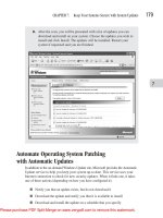
Configure Error-Checking Options
You can configure how Excel handles errors in worksheets by choosing Tools | Options and
selecting and clearing the check boxes as appropriate on the Error Checking tab of the Options
dialog box (Figure 8-2). Clear the Enable Background Error Checking check box if you want to
disable error checking altogether. Otherwise, use the options in the Rules section of the tab to
specify which rules to apply to your worksheets. (By default, Excel applies most of them.)
If you enter many formulas in your worksheets manually, you may find the Inconsistent
Formula in Region option useful for identifying inconsistencies in otherwise consistent ranges of
formulas.
The Reset Ignored Errors button on the Error Checking tab of the Options dialog box
lets you tell Excel that you want to see even those errors that you (or someone else)
have specifically ignored. You may want to use this option when you receive a workbook
from someone else and need to make sure it doesn’t contain any hidden errors that that
person has ignored.
178 How to Do Everything with Microsoft Office Excel 2003
HowTo-Tght (8) / How to Do Everything with Microsoft Office Excel 2003 / Hart-Davis / 3071-1 / Chapter 8
P:\010Comp\HowTo8\071-1\ch08.vp
Thursday, August 28, 2003 12:01:36 PM
Color profile: Generic CMYK printer profile
Composite Default screen
8
When Excel identifies an error that contravenes a rule that’s selected, it displays a green
triangle in the upper-left corner of the affected cell. Select the cell to display a Smart Tag, and
then click the Smart Tag to display a menu that explains the problem and offers possible solutions:
Audit Formulas and Check for Errors Manually
If you turn off Excel’s error checking, it’s a good idea to check your worksheets manually for
errors; if you use error checking, you may still want to check manually to ensure that you haven’t
ignored any cells flagged with green triangles.

CHAPTER 8: Create Formulas to Perform Custom Calculations 179
HowTo-Tght (8) / How to Do Everything with Microsoft Office Excel 2003 / Hart-Davis / 3071-1 / Chapter 8
FIGURE 8-2 Configure error-checking options on the Error Checking tab of the Options
dialog box.
P:\010Comp\HowTo8\071-1\ch08.vp
Thursday, August 28, 2003 12:01:36 PM
Color profile: Generic CMYK printer profile
Composite Default screen
You’ll see an example of checking for errors manually in a minute. But first, let’s look at the
formula auditing commands that Excel offers, because you’ll often need to use these to track
down errors.
Use the Formula Auditing Commands to Track Down Errors
The commands on the Formula Auditing toolbar (Figure 8-3) and the Tools | Formula Auditing
submenu enable you to track down errors in your formulas more quickly. The Formula Auditing
submenu offers many of the same options as the Formula Auditing toolbar, but the toolbar tends
to be easier to use.
You’ll see most of the Formula Auditing toolbar’s buttons in action in the next sections.
These buttons (which you won’t see in action) need only brief explanation:
■
The New Comment button inserts a new comment attached to the active cell.
■
The Show Watch Window button displays the Watch window (discussed in “Monitor
Calculations with the Watch Window” in Chapter 7).
Trace the Precedents or Dependents of a Cell
To determine which cells a particular value is derived from, you can select the cell and examine
its formula in the Formula bar. But doing this for any number of cells, to check the derivation of
a formula that seems to be giving an incorrect result, is tedious and time consuming. To help you,
Excel provides tools for tracing a cell’s precedents (the cells used to make up the value in this
cell) and dependents (the cells that use this cell in their formulas).
Click the Trace Precedents button on the Formula Auditing toolbar (or choose Tools |

Formula Auditing | Trace Precedents) to make Excel display an arrow to show which cells were
180 How to Do Everything with Microsoft Office Excel 2003
HowTo-Tght (8) / How to Do Everything with Microsoft Office Excel 2003 / Hart-Davis / 3071-1 / Chapter 8
FIGURE 8-3 Use the controls on the Formula Auditing toolbar to track down errors in
formulas.
Remove All Arrows Clear Validation Circles
Trace Precedents Trace Dependents Trace Error Evaluate Formula
Error Checking Remove Dependent Arrows Circle Invalid Data
Remove Precedent Arrows New Comment Show Watch Window
P:\010Comp\HowTo8\071-1\ch08.vp
Thursday, August 28, 2003 12:01:36 PM
Color profile: Generic CMYK printer profile
Composite Default screen
8
CHAPTER 8: Create Formulas to Perform Custom Calculations 181
HowTo-Tght (8) / How to Do Everything with Microsoft Office Excel 2003 / Hart-Davis / 3071-1 / Chapter 8
used to create the value in the active cell. In this illustration, you can see that the range G2:G6
makes up the value in cell G7:
Click the Trace Precedents button again to display the precedents of those cells if necessary.
In this illustration, the topmost arrow shows that cells E2 and F2 make up the value in cell G2,
and the four arrows beneath it show that the next four rows perform corresponding
calculations—E3 and F3 make up G3, and so on:
If your formulas go further, as the ones in the example do, you can pursue them back to their
origins by clicking the Trace Precedents button once more for each step. This illustration shows
the next (and final) stage of the formula:
You can remove precedent arrows one set at a time by clicking the Remove Precedent
Arrows button. So if Excel is displaying three stages of precedents (as in the example), the first
P:\010Comp\HowTo8\071-1\ch08.vp
Thursday, August 28, 2003 12:01:37 PM
Color profile: Generic CMYK printer profile

Composite Default screen
click removes the third stage, the second click removes the second stage, and the third click
removes the first stage.
To get rid of all precedent and dependent arrows instantly, click the Remove All Arrows
button or choose Tools | Formula Auditing | Remove All Arrows.
Instead of working backwards through a formula by tracing precedents, you may need to see
which calculations a particular value is used in. To do so, trace its dependents by clicking the
Trace Dependents button (or choosing Tools | Formula Auditing | Trace Dependents). Each click
displays one stage of calculation. These illustrations show the stages of a calculation in
succession:
You can remove dependent arrows one set at a time by clicking the Remove Dependent
Arrows button.
If a precedent or dependent cell is on another worksheet in the same workbook or a different
workbook, Excel displays an arrow to a small worksheet symbol:
182 How to Do Everything with Microsoft Office Excel 2003
HowTo-Tght (8) / How to Do Everything with Microsoft Office Excel 2003 / Hart-Davis / 3071-1 / Chapter 8
P:\010Comp\HowTo8\071-1\ch08.vp
Thursday, August 28, 2003 12:01:37 PM
Color profile: Generic CMYK printer profile
Composite Default screen