Microsoft Excel 2010: Data Analysis and Business Modeling phần 6 ppt

Chapter 42 Summarizing Data by Using Descriptive Statistics 345
The new Excel 2010 function RANK.AVG has the same syntax as the other RANK functions,
but in the case of ties, RANK.AVG returns the average rank for all tied data points. For
example, since the two scores of 98 ranked third and fourth, RANK.AVG returns 3.5 for each.
I generated the average ranks by copying the formula RANK.AVG(C4,$C$4:$C$62,0) from E4
to E5:E62.
What is the trimmed mean of a data set?
Extreme skewness in a data set can distort the mean of the data set. In these situations,
people usually use median as a measure of the data set’s typical value. The median, however,
is unaffected by many changes in the data. For example, compare the following two data
sets:
Set 1: –5, –3, 0, 1, 3, 5, 7, 9, 11, 13, 15
Set 2: –20, –18, –15, –10, –8, 5, 6, 7, 8, 9, 10
These data sets have the same median (5), but the second data set should have a lower
“typical” value than the rst. The Excel TRIMMEAN function is less distorted by extreme
values than the AVERAGE function, but it is more inuenced by extreme values than the
median. The formula =TRIMMEAN(range,percent) computes the mean of a data set after
deleting the data points at the top percent divided by 2 and bottom percent divided by
2. For example, applying the TRIMMEAN function with percent=10% converts the mean
after deleting the top 5 percent and bottom 5 percent of the data. In cell F3 of the le
Trimmean.xlsx, the formula =TRIMMEAN(C4:C62,.10) computes the mean of the scores in
C4:C62 after deleting the three highest and three lowest scores. (The result is 90.04.) In cell
F4, the formula =TRIMMEAN(C4:C62,.05) computes the mean of the scores in C4:C62 after
deleting the top and bottom scores. This calculation occurs because .05*59=2.95 would in-
dicate the deletion of 1.48 of the largest observations and 1.48 of the smallest. Rounding off
1.48 results in deleting only the top and bottom observations. (See Figure 42-7.)
When I select a range of cells, is there an easy way to get a variety of statistics that
describes the data in those cells?
To see the solution to this question, select the cell range C4:C36 in the le Trimmean.xlsx. In
the lower-right corner of your screen, the Excel status bar displays a cornucopia of statistics
describing the numbers in the selected cell range. (See Figure 42-8.) For example, for the cell

range C4:C36, the mean is 90.39, there are 33 numbers, the smallest value is 80, and the larg-
est value is 100. If you right-click the status bar, you can change the displayed set of statistics.
FIGURE 42-8 Statistics shown on the status bar.
346 Microsoft Excel 2010: Data Analysis and Business Modeling
Why do nancial analysts often use the geometric mean to summarize the average return
on a stock?
The le Geommean.xlsx contains the annual returns of two ctitious stocks. (See Figure 42-9.)
FIGURE 42-9 Geometric mean.
Cell C9 indicates that the average annual return on Stock 1 is 5 percent and the average
annual return on Stock 2 is 10 percent. This would seem to indicate that Stock 2 is a better
investment. If you think about it, however, what will probably happen with Stock 2 is that one
year you will lose 50 percent and the next gain 70 percent. This means that every two years
$1.00 becomes 1(1.7)(.5)=.85. Because Stock 1 never loses money, you know that it is clearly
the better investment. Using the geometric mean as a measure of average annual return
helps to correctly conclude that Stock 1 is the better investment. The geometric mean of n
numbers is simply the nth root of the product of the numbers. For example, the geometric
mean of 1 and 4 is the square root of 4 (2), whereas the geometric mean of 1, 2, and 4 is the
cube root of 8 (also 2). To use the geometric mean to calculate an average annual return on
an investment, you add 1 to each annual return and take the geometric mean of the resulting
numbers. Then subtract 1 from this result to obtain an estimate of the stock’s average annual
return.
The formula =GEOMMEAN(range) nds the geometric mean of numbers in a range. So, to
estimate the average annual return on each stock, you proceed as follows:
1. Compute 1+each annual return by copying from C12 to C12:D15 the formula =1+C5.
2. Copy from C16 to D16 the formula =GEOMEAN(C12:C15)–1.
The annual average return on Stock 1 is estimated to be 5 percent, and the annual average
return on Stock 2 is –7.8 percent. Note that if Stock 2 yields the mean return of –7.8 percent
during two consecutive years, $1 becomes 1(1–.078)
2
=.85, which agrees with common sense.

Chapter 42 Summarizing Data by Using Descriptive Statistics 347
Problems
1. Use the data in the le Stock.xlsx to generate descriptive statistics for Intel and GE
stock.
2. Use your answer to Problem 1 to compare the monthly returns on Intel and GE stock.
3. City Power & Light produces voltage-regulating equipment in New York and ships the
equipment to Chicago. A voltage regulator is considered acceptable if it can hold a
voltage of 25–75 volts. The voltage held by each unit is measured in New York before
each unit is shipped. The voltage is measured again when the unit arrives in Chicago. A
sample of voltage measurements from each city is given in the le Citypower.xlsx.
❑
Using descriptive statistics, comment on what you have learned about the voltage
held by units before and after shipment.
❑
What percentage of units are acceptable before and after shipping?
❑
Do you have any suggestions about how to improve the quality of City Power &
Light’s regulators?
❑
Ten percent of all New York regulators have a voltage exceeding what value?
❑
Five percent of all New York regulators have a voltage less than or equal to what
value?
4. In the le Decadeincome.xlsx, you are given a sample of incomes (in thousands of
1980 dollars) for a set of families sampled in 1980 and 1990. Assume that these families
are representative of the whole United States. Republicans claim that the country was
better off in 1990 than in 1980 because average income increased. Do you agree?
5. Use descriptive statistics to compare the annual returns on stocks, T-Bills, and corporate
bonds. Use the data contained in the le Historicalinvest.xlsx.
6. In 1970 and 1971, eligibility for the U.S. armed services draft was determined on the

basis of a draft lottery number. The number was determined by birth date. A total of
366 balls, one for each possible birth date, were placed in a container and shaken. The
rst ball selected was given the number 1 in the lottery, and so on. Men whose birth-
days corresponded to the lowest numbers were drafted rst. The le Draftlottery.xlsx
contains the actual results of the 1970 and 1971 drawings. For example, in the 1970
drawing, January 1 received the number 305. Use descriptive statistics to demonstrate
that the 1970 draft lottery was not random and the 1971 lottery was random (Hint: Use
the AVERAGE and MEDIAN functions to compute the mean and median lottery number
for each month.)
348 Microsoft Excel 2010: Data Analysis and Business Modeling
7. The le Jordan.xlsx gives the starting salaries (hypothetical) of all 1984 geography
graduates from the University of North Carolina (UNC). What is your best estimate of a
“typical” starting salary for a geography major? In reality, the major at UNC having the
highest average starting salary in 1984 was geography because the great basketball
player Michael Jordan was a geography major!
8. Use the LARGE or SMALL function to sort the annual stock returns in the le
Historicalinvest.xlsx. What advantage does this method of sorting have over clicking the
Sort button?
9. Compare the mean, median, and trimmed mean (trimming 10 percent of the
data) of the annual returns on stocks, T-Bills, and corporate bonds given in the le
Historicalinvest.xlsx.
10. Use the geometric mean to estimate the mean annual return on stocks, bonds, and
T-Bills in the le Historicalinvest.xlsx.
11. The le Dow.xlsx contains monthly returns on the 30 Dow stocks during the last 20
years. Use this data to determine the three stocks with the largest mean monthly
returns.
12. Using the Dow.xlsx data again, determine the three stocks with the most risk or
variability.
13. Using the Dow.xlsx data, determine the three stocks with the highest skew.
14. Using the Dow.xlsx data, how do the trimmed-mean returns (trim off 10 percent of the

returns) differ from the overall mean returns?
15. The le Incomedata.xlsx contains incomes of a representative sample of Americans in
the years 1975, 1985, 1995, and 2005. Describe how U.S. personal income has changed
over this time period.
16. The le Coltsdata.xlsx contains yards gained by the 2006 Indianapolis Colts on each
rushing and passing play. Describe how the outcomes of rushing plays and passing
plays differ.
349
Chapter 43
Using PivotTables and Slicers to
Describe Data
Questions answered in this chapter:
■
What is a PivotTable?
■
How can I use a PivotTable to summarize grocery sales at several grocery stores?
■
What PivotTable layouts are available in Excel 2010?
■
Why is a PivotTable called a PivotTable?
■
How can I easily change the format in a PivotTable?
■
How can I collapse and expand elds?
■
How do I sort and lter PivotTable elds?
■
How do I summarize a PivotTable by using a PivotChart?
■
How do I use the Report Filter section of the PivotTable?

■
How do Excel 2010 slicers work?
■
How do I add blank rows or hide subtotals in a PivotTable?
■
How do I apply conditional formatting to a PivotTable?
■
How can I update my calculations when I add new data?
■
I work for a small travel agency for which I need to mass-mail a travel brochure. My
funds are limited, so I want to mail the brochure to people who spend the most money
on travel. From information in a random sample of 925 people, I know the gender, the
age, and the amount these people spent on travel last year. How can I use this data to
determine how gender and age inuence a person’s travel expenditures? What can I
conclude about the type of person to whom I should mail the brochure?
■
I’m doing market research about Volvo Cross Country Wagons. I need to determine
what factors inuence the likelihood that a family will purchase a station wagon. From
information in a large sample of families, I know the family size (large or small) and the
family income (high or low). How can I determine how family size and income inuence
the likelihood that a family will purchase a station wagon?
350 Microsoft Excel 2010: Data Analysis and Business Modeling
■
I work for a manufacturer that sells microchips globally. I’m given monthly actual and
predicted sales for Canada, France, and the United States for Chip 1, Chip 2, and Chip 3.
I’m also given the variance, or difference, between actual and budgeted revenues.
For each month and each combination of country and product, I’d like to display the
following data: actual revenue, budgeted revenue, actual variance, actual revenue as
a percentage of annual revenue, and variance as a percentage of budgeted revenue.
How can I display this information?

■
What is a calculated eld?
■
How do I use a report lter or slicer?
■
How do I group items in a PivotTable?
■
What is a calculated item?
■
What is “drilling down”?
■
I often have to use specic data in a PivotTable to determine prot, such as the April
sales in France of Chip 1. Unfortunately, this data moves around when new elds are
added to my PivotTable. Does Excel have a function that enables me to always extract
April’s Chip 1 sales in France from the PivotTable?
Answers to This Chapter’s Questions
What is a PivotTable?
In numerous business situations, you need to analyze, or “slice and dice,” your data to gain
important insights. Imagine that you sell different grocery products in different stores at
different points in time. You might have hundreds of thousands of data points to track.
PivotTables let you quickly summarize your data in almost any way imaginable. For example,
for your grocery store data, you could use a PivotTable to quickly determine the following:
■
Amount spent per year in each store on each product
■
Total spending at each store
■
Total spending for each year
In a travel agency, as another example, you might slice data so that you can determine
whether the average amount spent on travel is inuenced by age or gender or by both

factors. In analyzing automobile purchases, you’d like to compare the fraction of large
families that buy a station wagon to the fraction of small families that purchase a station
wagon. For a microchip manufacturer, you’d like to determine total Chip 1 sales in France,
for example, during April, and so on. A PivotTable is an incredibly powerful tool that you
can use to slice and dice data. The easiest way to understand how a PivotTable works is
to walk through some carefully constructed examples, so let’s get started! I’ll begin with
Chapter 43 Using PivotTables and Slicers to Describe Data 351
an introductory example and then illustrate many advanced PivotTable features through
subsequent examples.
Note Excel 2010 contains a new feature called slicers that make it much easier to use PivotTables
to examine your data from many perspectives. I discuss slicers later in the chapter.
How can I use a PivotTable to summarize grocery sales at several grocery stores?
The Data worksheet in the le Groceriespt.xlsx contains more than 900 rows of sales data.
(See Figure 43-1.) Each row contains the number of units sold and revenue of a product at a
store, as well as the month and year of the sale. The product group (either fruit, milk, cereal,
or ice cream) is also included. You would like to see a breakdown of sales during each year of
each product group and product at each store. You would also like to be able to show this
breakdown during any subset of months in a given year (for example, what the sales were
during January–June).
FIGURE 43-1 Data for the grocery PivotTable example.
Before creating a PivotTable, you must have headings in the rst row of your data. Notice
that the grocery data contains headings (Year, Month, Store, Group, Product, Units, and
Revenue) in row 2. Place your cursor anywhere in the data, and then click PivotTable in
the Tables group on the Insert tab. Excel opens the Create PivotTable dialog box, shown in
Figure 43-2, and makes an assumption about your data range. (In this case, Excel correctly
guessed that the data range was C2:I924.) By selecting Use An External Data Source, you can
also refer to a database as a source for a PivotTable.
352 Microsoft Excel 2010: Data Analysis and Business Modeling
FIGURE 43-2 The Create PivotTable dialog box.
After you click OK, you see the PivotTable Field List shown in Figure 43-3.

FIGURE 43-3 The PivotTable Field List.
You ll in the PivotTable Field List by dragging PivotTable headings, or elds, into the boxes,
or zones. This step is critical to ensuring that the PivotTable will summarize and display the
data in the manner you want. The four zones are as follows:
■
Row Labels Fields dragged here are listed on the left side of the table in the order
in which they are added to the box. For example, I dragged to the Row Labels box the
elds Year, Group, Product, and Store, in that order. This causes Excel to summarize
data rst by year, then for each product group within a given year, then by product
within each group, and nally each product by store. You can at any time drag a eld to
a different zone or reorder the elds within a zone by dragging a eld up or down in a
zone or by clicking the arrow to the right of the eld label.
Chapter 43 Using PivotTables and Slicers to Describe Data 353
■
Column Labels Fields dragged here have their values listed across the top row of the
PivotTable. To start out this example, we have no elds in the Column Labels zone.
■
Values Fields dragged here are summarized mathematically in the table. I dragged
Units and Revenue (in that order) to this zone. Excel tries to guess what kind of cal-
culation you want to perform on a eld. In this example, Excel guesses that Revenue
and Units should be summed, which happens to be correct. If you want to change the
method of calculation for a data eld to an average, a count, or something else, simply
click the data eld and choose Value Field Settings. I give an example of how to use the
Value Field Settings command later in the chapter.
■
Report Filter Beginning in Excel 2007, Report Filter is the new name for the old Page
Field area. For elds dragged to the Report Filter area, you can easily pick any subset of
the eld values so that the PivotTable shows calculations based only on that subset. In
this example, I dragged Month to the Report Filter area. That lets me easily select any
subset of months, for example January–June, and the calculations are based on only

those months. Slicers in Excel 2010 make report lters virtually obsolete.
The completed PivotTable Field List is shown in Figure 43-4. The resulting PivotTable is shown
in Figure 43-5 and in the All Row Fields worksheet of the workbook Groceriespt.xlsx. In row 6,
you can see that 233,161 units were sold for $702,395.82 in 2007.
Tip Here is some advice about navigating workbooks (like the one in this example) containing
many worksheets. In the lower-right corner of the Excel window (to the left of the worksheet
names), you will see four arrows. Clicking the left-most arrow takes you to the rst worksheet;
clicking the right-most arrow shows the last worksheet; and clicking the other arrows moves you
one worksheet to the left or right.
Note To see the eld list, you need to be in a eld in the PivotTable. If you do not see the eld
list, right-click any cell in the PivotTable and select Show Field List.
FIGURE 43-4 Completed PivotTable Field List.
354 Microsoft Excel 2010: Data Analysis and Business Modeling

FIGURE 43-5 The Grocery PivotTable in compact form.
What PivotTable layouts are available in Excel 2010?
The PivotTable layout shown in Figure 43-5 is called the compact form. In the compact form,
the row elds are shown one on top of another. To change the layout, rst place your cursor
anywhere within the table. On the Design tab, in the Layout Group, click Report Layout, and
choose one of the following: Show In Compact Form (see Figure 43-5), Show In Outline Form
(see Figure 43-6 and the Outline Form worksheet), or Show In Tabular Form (Figure 43-7 and
the Tabular Form worksheet).
FIGURE 43-6 The outline format.
Chapter 43 Using PivotTables and Slicers to Describe Data 355
FIGURE 43-7 The tabular format.
Why is a PivotTable called a PivotTable?
You can easily pivot elds from a row to a column and vice versa to create a different layout.
For example, by dragging the Year eld to the Column Labels box, you create the PivotTable
layout shown in Figure 43-8. (See the Years Column worksheet.)
FIGURE 43-8 The Years eld pivoted to the column eld.

How can I easily change the format in a PivotTable?
If you want to change the format of an entire column eld, simply double-click the column
heading and select Number Format from the Value Field Settings dialog box. Then apply the
format you want. For example, in the Formatted $s worksheet, I formatted the Revenue eld
as currency by double-clicking the Sum Of Revenue heading and applying a currency format.
You can also change the format of a value eld by clicking the arrow to the right of the Value
356 Microsoft Excel 2010: Data Analysis and Business Modeling
eld in the PivotTable Field List. Select Value Field Settings followed by Number Format, and
then you can reformat the column as you want it.
From any cell in a PivotTable, you can select the Design tab on the ribbon to reveal many
PivotTable styles.
How can I collapse and expand elds?
Expanding and collapsing elds (a feature introduced in Excel 2007) is a great advantage in
PivotTables. In Figure 43-5, you see minus (–) signs by each year, group, and product. Clicking
the minus sign collapses a eld and changes the sign to a plus (+) sign. Clicking the plus sign
expands the eld. For example, if you click the minus sign by cereal in any cell in column A,
you will nd that in each year, cereal is contracted to one row, and the various cereals are no
longer listed. See Figure 43-9 and the Cerealcollapse worksheet. Clicking the plus sign in cell
A6 brings back the detailed or expanded view listing all the cereals.
FIGURE 43-9 The cereal eld collapsed.
You can also expand or contract an entire eld. Go to any row containing a member of that
eld, and select PivotTable Tools Options on the ribbon. In the Active Field group, click either
the green Expand Entire Field button (labeled with a plus sign) or the red Contract Entire
Field button (labeled with a minus sign). (See Figure 43-10.)
FIGURE 43-10 The Expand Entire Field and Contract Entire Field buttons.
Chapter 43 Using PivotTables and Slicers to Describe Data 357
For example, suppose you simply want to see for each year the sales by product group.
Pick any cell containing a group’s name (for example, A6), select PivotTable Tools Options
on the ribbon, and click the Collapse Entire Field button. You will see the result shown in
Figure 43-11 (the Groups Collapsed worksheet). Selecting the Expand Entire Field button

brings you back to the original view.
FIGURE 43-11 The Group eld collapsed.
How do I sort and lter PivotTable elds?
In Figure 43-5, the products are listed alphabetically within each group. For example,
chocolate is the rst type of milk listed. If you want the products to be listed in reverse
alphabetical order, simply move the cursor to any cell containing a product (for example, A7
in the All Row Fields worksheet) and click the drop-down arrow to the right of the Row Labels
entry in A5. You will see the list of ltering options shown in Figure 43-12. Selecting Sort Z To
A would list whole milk rst for milk, plums for fruit, and so on.
Initially, our PivotTable displays results rst from 2007, then 2006, and then 2005. If you want
to see the data for 2005 rst, move the cursor to any cell containing a year (for example, A5),
and choose Sort Smallest To Largest from the available options.
At the bottom of the ltering options dialog box, you can also select any subset of products
to be displayed. You may want to rst clear Select All and then select the products you
want to show.
358 Microsoft Excel 2010: Data Analysis and Business Modeling
FIGURE 43-12 PivotTable ltering options for the Product eld.
For another example of ltering, look at the Data worksheet in the le Ptcustomers.xlsx,
shown in Figure 43-13. The worksheet data contains for each customer transaction the
customer number, the amount paid, and the quarter of the year in which payment was
received. After dragging Customer to the Row Labels box, Quarter to the Column Labels box,
and Paid to the Values box, the PivotTable shown in Figure 43-14 is displayed. (See the Ptable
worksheet in the Pcustomers.xlsx le.)
FIGURE 43-13 The Customer PivotTable data.
Chapter 43 Using PivotTables and Slicers to Describe Data 359
FIGURE 43-14 The Customer PivotTable.
Naturally, you might like to show a list of just your top 10 customers. To obtain this layout,
simply click the Row Labels arrow and select Value Filters. Then choose Top 10 items to ob-
tain the layout shown in Figure 43-15 (see the Top 10 cus worksheet). Of course, by selecting
Clear Filter, you can return to the original layout.

FIGURE 43-15 Top 10 customers.
Suppose you simply want to see the top customers that generate 50 percent of your revenue.
Select the Row Labels ltering icon, select Value Filters, Top 10, and ll in the dialog box as
shown in Figure 43-16.
360 Microsoft Excel 2010: Data Analysis and Business Modeling
FIGURE 43-16 Conguring the Top 10 Filter dialog box to show customers generating 50 percent of revenue.
The resulting PivotTable is in the Top half worksheet and shown in Figure 43-17. As you can
see, the top 14 customers generate a little more than half of the revenue.
FIGURE 43-17 The top customers generating half of the revenues.
Now let’s suppose you want to sort your customers by Quarter 1 revenue. (See the Sorted q1
worksheet.) Right-click anywhere in the Quarter 1 column, point to Sort, and then click Sort
Largest To Smallest. (See Figure 43-18.) The resulting PivotTable is shown in Figure 43-19. Note
that Customer 13 paid the most in Quarter 1, Customer 2 paid the second most, and so on.
FIGURE 43-18 Sorting on the Quarter 1 column.
Chapter 43 Using PivotTables and Slicers to Describe Data 361
FIGURE 43-19 Customers sorted on Quarter 1 revenue.
How do I summarize a PivotTable by using a PivotChart?
Excel makes it easy to visually summarize PivotTables by using PivotCharts. The key to laying
out the data the way you want it in a PivotChart is to sort data and collapse or expand
elds. In the grocery example, suppose you want to summarize the trend over time of each
food group’s unit sales. (See the Chart 1 worksheet in the le Groceriespt.xlsx.) You should
move the Year eld to a column eld and delete Revenue as a values eld. You also need
to collapse the entire Group eld in the Row Labels zone. Now you are ready to create a
PivotChart. Simply click anywhere inside the table, and select Options, PivotChart. Now
pick the chart type you want to create. I chose the fourth Line Graph option, which displays
the chart in Figure 43-20. The chart shows that milk sales were highest in 2005 and lowest
in 2006.
362 Microsoft Excel 2010: Data Analysis and Business Modeling
FIGURE 43-20 PivotChart for unit group sales trend.
How do I use the Report Filter section of the PivotTable?

Recall that I placed Months in the Report Filter section of the table. To see how to use a
report lter, suppose that you want to summarize sales for the months January–June. By
clicking the Filter icon in cell B2 of the First 6 months worksheet, you can select January–June.
This results in the PivotTable shown in Figure 43-21, which summarizes the number of units
sold by product, group, and year for the months January–June.
FIGURE 43-21 A PivotTable summarizing January–June sales.
Chapter 43 Using PivotTables and Slicers to Describe Data 363
How do Excel 2010 slicers work?
The problem with a report lter is that a viewer of the PivotTable shown in Figure 43-21
cannot easily see that the table summarizes January–June sales. Excel’s 2010 slicer feature
solves this problem. To create a slicer for any of the columns of data used to generate your
PivotTable, place your cursor anywhere in the PivotTable, and then click Slicer on the ribbon’s
Insert tab. In the worksheet Slicers of the le Groceriespt.xlsx, I selected Slicer from the Insert
menu. Then I selected the Month and Product elds to create slicers for Month and Product.
Using a given slicer, you can select any subset of possible values to be used in creating your
table.In the Month slicer, I selected (one at a time, while holding down the Ctrl key) the
months January through June. I did nothing to the Product slicer, so the data is based on
January–June sales. The slicers are shown in Figure 43-22.
FIGURE 43-22 Example of slicers for the Month and Product elds.
If you click in a slicer, you see formatting options that allow you to change its look.
How do I add blank rows or hide subtotals in a PivotTable?
If you want to add a blank row between each grouped item, select PivotTable Tools Design
on the ribbon, click Blank Rows, and then click Insert Blank Line After Each Item. If you want
to hide subtotals or grand totals, select PivotTable Tools Design, and then select Subtotals or
Grand Totals. After adding blank rows and hiding all totals, I obtained the table in the Blank
rows no totals worksheet, shown in Figure 43-23. After right-clicking in any PivotTable cell,
you can select PivotTable Options to open the PivotTable Options dialog box. In this dialog
box, you can replace empty cells by using any character, such as an underscore (_), or by
using a 0.
FIGURE 43-23 Grocery PivotTable without totals.

364 Microsoft Excel 2010: Data Analysis and Business Modeling
How do I apply conditional formatting to a PivotTable?
Suppose you want to apply data bars to the Units column in the grocery PivotTable. One
problem you’ll encounter is that subtotals and grand totals will have large data bars and also
make the other
data bars smaller than they should be. It’s better to have the data bars apply
to all product sales, not the subtotals and grand totals. (See the Cond form worksheet of
workbook Groceriespt.xlsx.) To apply the data bars to only the unit sales by product, begin
by placing the cursor in a cell containing a product (for example, chocolate milk in B8), and
then select the Sum Of Units column data (the cell range B7:B227). On the Home tab, click
Conditional Formatting followed by Data Bars, and then choose More Rules. You will see the
New Formatting Rule dialog box shown in Figure 43-24.
FIGURE 43-24 New Formatting Rule dialog box for using conditional formatting with PivotTables.
By selecting All Cells Showing “Sum of Units” Values For “Product”, you can ensure that
data bars apply only to cells listing unit sales for products, as you can see in the Cond form
worksheet and Figure 43-25.
Chapter 43 Using PivotTables and Slicers to Describe Data 365
FIGURE 43-25 Data bars for a PivotTable.
How can I update my calculations when I add new data?
If the data in your original set of rows changes, you can update your PivotTable to include the
data changes by right-clicking the table and selecting Refresh. You can also select Refresh
after choosing Options.
If you want data you add to be automatically included in your PivotTable calculations when
you refresh it, you should name your original data set as a table by selecting it with Ctrl+T.
(See Chapter 26, “Tables,” for more information.)
If you want to change the range of data used to create a PivotTable, you can always select
Change Data Source on the Options tab. You can also move the table to a different location
by selecting Move PivotTable.
I work for a small travel agency for which I need to mass-mail a travel brochure My
funds are limited, so I want to mail the brochure to people who spend the most money

on travel From information in a random sample of 925 people, I know the gender, the
age, and the amount these people spent on travel last year How can I use this data to
determine how gender and age inuence a person’s travel expenditures? What can I
conclude about the type of person to whom I should mail the brochure?
To understand this data, you need to break it down as follows:
■
Average amount spent on travel by gender
■
Average amount spent on travel for each age group
■
Average amount spent on travel by gender for each age group
366 Microsoft Excel 2010: Data Analysis and Business Modeling
The data is included on the Data worksheet in the le Traveldata.xlsx, and a sample is shown
in Figure 43-26. For example, the rst person is a 44-year-old male who spent $997 on travel.
Let’s rst get a breakdown of spending by gender. Begin by selecting Insert PivotTable. Excel
extracts the range A2:D927. After clicking OK, put the cursor in the table so that the eld list
appears. Next, drag the Gender column to the Row Labels zone and drag Amount Spent On
Travel to the Values zone. This results in the PivotTable shown in Figure 43-27.
You can tell from the heading Sum Of Amount Spent On Travel that you are summarizing the
total amount spent on travel, but you actually want the average amount spent on travel by
men and women. To calculate these quantities, double-click Sum Of Amount Spent On Travel
and then select Average from the Value Field Settings dialog box, shown in Figure 43-28.
FIGURE 43-26 Travel agency data showing amount spent on travel, age, and gender.
FIGURE 43-27 PivotTable summarizing the total travel expenditures by gender.
FIGURE 43-28 You can select a different summary function in the Value Field Settings dialog box.
Chapter 43 Using PivotTables and Slicers to Describe Data 367
You now see the results shown in Figure 43-29.
FIGURE 43-29 Average travel expenditures by gender.
On average, people spend $908.13 on travel. Women spend an average of $901.16, whereas
men spend $914.99. This PivotTable indicates that gender has little inuence on the propen-

sity to travel. By clicking the Row Labels arrow, you can show just male or female results.
Now you want to see how age inuences travel spending. To remove Gender from the
PivotTable, simply click Gender in the Row Labels portion of the PivotTable Field List and
remove it from the Row Labels area. Then, to break down spending by age, drag Age to the
row area. The PivotTable now appears as it’s shown in Figure 43-30.
FIGURE 43-30 PivotTable showing the average travel expenditures by age.
Age seems to have little effect on travel expenditures. In fact, this PivotTable is pretty useless
in its present state. You need to group data by age to see any trends. To group the results by
age, right-click anywhere in the Age column and choose Group. In the Grouping dialog box,
you can designate the interval by which to dene an age group. By using 10-year increments,
you obtain the PivotTable shown in Figure 43-31.
On average, 25–34 year olds spend $935.84 on travel, 55–64 year olds spend $903.57 on
travel, and so on. This information is more useful, but it still indicates that people of all
ages tend to spend about the same amount on travel. This view of the data does not help
determine who you should mail your brochure to.
368 Microsoft Excel 2010: Data Analysis and Business Modeling
FIGURE 43-31 Use the Group And Show Detail command to group detailed records.
Finally, let’s get a breakdown of average travel spending by age, for men and women
separately. All you have to do is drag Gender to the Column Labels zone of the eld list
resulting in the PivotTable shown in Figure 43-32 (see the Final Table worksheet).
FIGURE 43-32 Age/gender breakdown of travel spending.
Now we’re cooking! You can see that as age increases, women spend more on travel and
men spend less. Now you know who should get the brochure: older women and younger
men. As one of my students said, “That would be some kind of cruise!”
A graph provides a nice summary of this analysis. After moving the cursor inside the
PivotTable and choosing PivotChart, select the fourth option from Column Graphs. The result
is the chart shown in Figure 43-33. If you want to edit the chart further, select PivotChart
Tools. Then, for example, if you choose Layout, you can add titles to the chart and axis and
make other changes.
FIGURE 43-33 PivotChart for the age/gender travel expenditure breakdown.

Chapter 43 Using PivotTables and Slicers to Describe Data 369
Each age group spends approximately the same on travel, but as age increases, women
spend more than men. (If you want to use a different type of chart, you can change the chart
type by right-clicking the PivotChart and then choosing Chart Type.)
Notice that the bars showing expenditures by males decrease with age, and the bars
representing the amount spent by women increase with age. You can see why the PivotTables
that showed only gender and age data failed to unmask this pattern. Because half our sam-
ple population are men and half are women, we found that the average amount spent by
people does not depend on the age. (Notice that the average height of the two bars for each
age is approximately the same.) We also found that the average amount spent by men and
women was approximately the same. You can see this because, averaged over all ages, the
blue and red bars have approximately equal heights. Slicing and dicing the data simultane-
ously across age and gender does a much better job of showing you the real information.
I’m doing market research about Volvo Cross Country Wagons. I need to determine
what factors inuence the likelihood that a family will purchase a station wagon.
From information in a large sample of families, I know the family size (large or small)
and the family income (high or low). How can I determine how family size and income
inuence the likelihood that a family will purchase a station wagon?
In the le Station.xlsx, you can nd the following information:
■
Is the family size large or small?
■
Is the family’s income high or low?
■
Did the family buy a station wagon? Yes or No.
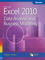
A sample of the data is shown in Figure 43-34 (see the Data worksheet). For example, the rst
family listed is a small, high-income family that did not buy a station wagon.
FIGURE 43-34 Data collected about income, family size, and the purchase of a station wagon.